Pattern Reconstruction from Near-Field Data Affected by 3D Probe Positioning Errors Collected via Planar-Wide Mesh Scanning

Abstract

An effective procedure to correct known 3D probe positioning errors affecting the near-field–far-field transformation (NF–FF) with non-conventional plane rectangular scanning, named planar wide-mesh scanning (PWMS), is developed in this paper. It relies on the non-redundant sampling representations of electromagnetic fields and related optimal sampling interpolation (OSI) expansions and has been devised when a quasi-planar antenna under test is considered as suitably modelled by either a double bowl or an oblate spheroid. Such an algorithm first makes use of the so-called k-correction to compensate for the errors occurring when the actual sampling points deviate from the acquisition plane and then adopts an iterative procedure to restore the NF samples at the points specified by the used non-redundant sampling representation from those obtained at the previous step and affected by 2D positioning errors. Finally, once the regularly arranged PWMS samples have been calculated, the NF data required to compute the classic plane-rectangular NF–FF transformation are accurately evaluated by using an effective 2D OSI algorithm. Several numerical results are presented in order to assess the effectiveness of the devised approach.

1. Introduction

Nowadays, the evaluation of the radiation features of an antenna under test (AUT) represents a crucial task to assure that the strict design specifications are fully satisfied. The simplest measurement strategy involves the direct far-field (FF) acquisition. To preserve the measurement accuracy from the influence of the surrounding environment, i.e., reflections from close objects, electromagnetic (EM) interferences, or weather conditions, it is convenient to characterize the AUT in a shielded and almost reflection free environment (anechoic chamber) well simulating the free-space propagation condition. However, direct measurements of the FF characteristics of AUTs with moderately large or even medium electrical sizes may be accurately carried out only in an expensive and very large anechoic chamber in order to fulfill the well-known FF distance requirements. Unfortunately, when the size of an anechoic chamber is limited, these constrains cannot be complied and, hence, only near-field (NF) measurements are possible. Obviously, a suitable NF–FF transformation technique is required to get the FF pattern reconstruction from the acquired NF data [1,2,3,4,5,6,7,8]. Spherical, cylindrical, and planar NF–FF transformation techniques are related to spherical, cylindrical, and planar NF scanning surfaces, respectively, and exploit the corresponding modal expansion of the AUT near field to calculate the FF pattern. In this framework, the NF–FF transformation with plane-rectangular (PR) scanning [9,10] results to be the simplest one in analytical and computational terms and may be appropriately used to get the characterization of high-gain antennas having pencil beam patterns substantially inside the solid angle defined by the edges of the AUT and those of the acquisition area. Moreover, since the alignment procedure in the PR facility is easily performed and the AUT is kept stationary during the acquisition process, such a scanning is mechanically simple too. Furthermore, the classic sampling strategy requires a sampling step constant along the scanner axes and bounded by λ/2, where λ is the wavelength at the working frequency. As a result, a huge amount of NF samples can be required. Clearly, the greater the amount of NF samples, the longer the related measurement time, which becomes longer and longer as the scanning plane sizes and/or the operating frequency increase. In order to conveniently reduce the needed NF measurements, NF–FF transformations using an innovative PR scanning strategy, called planar wide-mesh scanning (PWMS), have been developed and experimentally validated in [11] and [12], respectively, by properly exploiting the non-redundant sampling representations of the EM fields [13,14] to the voltage measured by the probe, which, according to [15], must be electrically small in order to have same spatial bandwidth as the field radiated by the AUT. This scanning technique allows a remarkable saving of measurement time as compared to classic PR scanning, since, as its name suggests, the sampling lattice meshes enlarge more and more on going away from the center of the scanning plane (see Figure 1). The collected PWMS samples are then interpolated via an effective interpolation scheme, based on the use of the optimal sampling interpolation (OSI) formulas, to reconstruct the PR data which allow the precise evaluation of the radiated pattern through the classic PR NF–FF transformation [10]. In particular, a spherical modelling has been used in [16], whilst an oblate spheroid and a double bowl, a surface built by two circular “bowls” having the same aperture but possibly not equal lateral bendings, have been adopted in [11,12] to model the antenna. These last modellings are particularly suitable for dealing with quasi-planar AUTs, since they make possible a significant reduction in the number of required NF data. Moreover, they make it possible to place the acquisition plane at a distance from the AUT which is smaller than one half its largest dimension, thus allowing the reduction in the error due to the truncation of the measurement plane.

Note that no hardware changes are needed in an existing PR facility to realize the PWMS and, thus, the same x–y scanner can be used to drive the probe to the required measurement points. Accordingly, the PWMS retains the same mechanical advantages and disadvantages as the PR scanning. Among these last, the finite resolution of the probe positioners and/or their imprecise control may make it very difficult to collect the NF samples at exactly the sampling points imposed by the adopted sampling representation. Furthermore, defects in the mechanical rails that drive the probe motion may introduce a deviation from the considered acquisition plane. Therefore, the NF acquisition may be corrupted by 3D positioning errors, which, in any case, can be accurately detected using a laser interferometric technique. It is clear that the same type of errors may also occur when the acquisition is made by robotic systems, whose application in this framework is spreading. In both cases, when increasing the operating frequency, it becomes more and more difficult to meet the required positioning accuracy.

To overcome the above issue, the approach proposed in [17], which is able to correct the phase error occurring when the actual sampling points deviate from the nominal acquisition plane and, accordingly, the named k-correction, is here used as a first step to compensate the 3D positioning errors. After that, a convenient and feasible strategy is to retrieve the samples correctly located at the points of the adopted sampling representation from those obtained at the previous step and now affected by 2D positioning errors, by using an effective iterative procedure [18,19,20,21,22,23,24,25]. The devised procedure converges only when it is possible to formulate a bijective relationship associating every correct (regular) sampling point with the nearest improperly positioned (irregular) one. A different approach, not suffering from the above constraints, is employing the singular value decomposition procedure to compute the regular PWMS samples from those corrupted by positioning errors [21,22,23,24,25,26,27,28]. Anyhow, to avoid a huge computational effort, such an approach can be adopted only if it is possible to split the retrieving of the regular samples in two independent 1D problems. It must be stressed that the positioning correction approaches in [18,19,20,21,22,23,24,25,26,27,28] can be applied only if the sampling points lie on the nominal measurement surface, since they are based on 2D non-redundant sampling representations. An exhaustive discussion on the reconstruction of the regular samples from the irregular ones and a related wide bibliography can be found in [18,22].

The article is organized as follows. In Section 2, a proper sampling representation of the voltage acquired by the probe on the scan plane is devised by properly exploiting the non-redundant representations of EM fields [13,14] and considering either an oblate spheroid or a double bowl as a modelling surface. A 2D OSI formula, which allows an accurate retrieving of the probe voltage at any point on the measurement plane from a reduced set of its samples, is also described in the same section. In Section 3, the devised multi-steps procedure to compensate the 3D probe positioning errors is explained. Many numerical results assessing the effectiveness of the proposed compensation approach are then presented in Section 4. Finally, concluding remarks are reported in Section 5.

2. PWMS Sampling Arrangement

The goal of this section is to describe the non-redundant sampling representation of the voltage detected by a small, non-directive, probe on the acquisition plane using a minimum number of PWMS samples, which is particularly suitable when dealing with quasi-planar AUTs.

To this end, let us assume that the measurement plane is d away from the AUT center, coincident with the origins O of the rectangular (x, y, z) and spherical (r, ϑ, ϕ) reference frames, both used for denoting an observation point P, and introduce another rectangular reference frame (x′, y′, z′) with its origin O′ at the measurement plane center to identify any point on the scanning plane.

According to the non-redundant representation of the EM field [13], an effective sampling representation can be obtained by considering the AUT as contained in a proper surface Σ, using an opportune parameter μ to describe any curve C on the plane external to Σ, and introducing the so called “reduced voltage” obtained by extracting a proper phase function ${\mathrm{e}}^{-\mathrm{j}\gamma (\mu )}$ from the expression of the voltages $V_y$ and $V_x$, measured by the probe and rotated probe. Such a reduced voltage,

$${\tilde{V}}_{x,y}(\mu )=V_{x,y}(\mu ){\mathrm{e}}^{\mathrm{j}\gamma (\mu )}$$

(1)

is a function spatially quasi-bandlimited to $W_{\mu }$, which, for the adopted probe, coincides practically with that of the AUT radiated field [15]. Such a function can be effectively approximated by a bandlimited one, provided that the associated bandlimitation error is minimized as much as possible. To this end, the bandwidth of the approximating function can be properly augmented to $\chi \prime W_{\mu }$, where $\chi \prime$ is an enlargement factor controlling the aliasing error and slightly greater than unity for electrically large antennas [13].

It is worth noting that the PWMS sampling points refer to the non-redundant sampling representation regarding two specific radial lines, namely, the x′- and y′-axes. In fact, as explained in the following, the sampling points falling out of the axes are obtained by intersecting the straight lines running parallel to the axes and passing through the sampling points on the axes (see Figure 1).

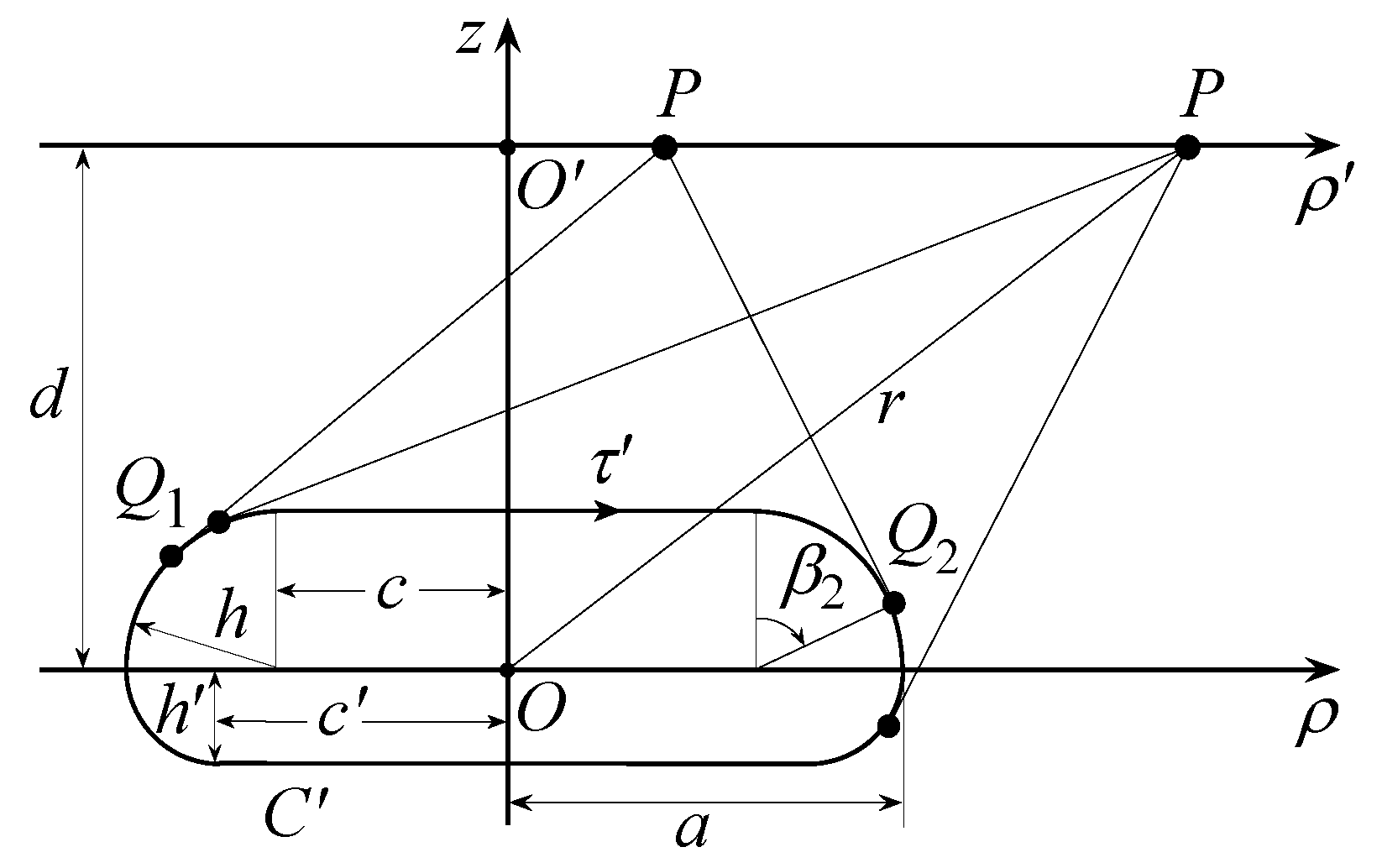
According to [13], when C is a radial line, as the $x\prime$ or $y\prime$ axis, by indicating with ${\tau }_{1,2}^{\prime }$ the arclength abscissas of the tangency points $Q_{1,2}$ on C’ (intersection curve of the meridian plane passing through P with Σ), with $\overline{P{Q}_1}$ and $\overline{P{Q}_2}$ the distances from P to $Q_{1,2}$, and choosing the bandwidth equal to

$$W_{\mu }=\frac{\ell \prime }{\lambda }$$

(2)

where $\ell \prime$ is the length of the curve C’, the optimal parameter and phase function are [13]:

$$\mu =\left(\pi /\ell \prime \right)\left[ \overline{P{Q}_1}-\overline{P{Q}_2}+{\tau }_1^{\prime }+{\tau }_2^{\prime }\right]$$

(3)

$$\gamma =\left(\pi /\lambda \right)\left[ \overline{P{Q}_1}+\overline{P{Q}_2}+{\tau }_1^{\prime }-{\tau }_2^{\prime }\right]$$

(4)

Note that the surface Σ surrounding the AUT has to be suitably chosen in order to derive an effective non-redundant representation. This surface must be regular and able to fit as much as possible the AUT actual geometry for reducing the volumetric redundancy and, thus, the number of needed sampling points. Indeed, as reported in [13], the total number NoS of NF samples at Nyquist step on a closed observation surface (also unbounded) enclosing the AUT is related to Σ through:

$$NoS\cong \frac{\mathrm{area} (\Sigma )}{{(\lambda /2)}^2}$$

(5)

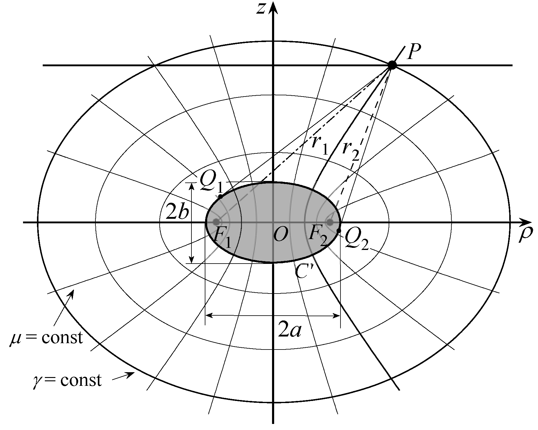
The AUT spherical modelling represents the simplest choice. However, its use to model a quasi-planar AUT gives rise to a volumetric redundancy, which reflects in a needless growth of the required samples. Accordingly, when quasi-planar AUTs need to be characterized, a better fitting of the AUT actual geometry can be obtained by using an oblate spheroid (see Figure 2a) or a double bowl (see Figure 2b). It should be pointed out that the relations (2)–(4) change depending on which surface Σ has been chosen for shaping the considered antenna. For reader’s convenience, their expressions for the oblate spheroid and the double bowl are reported in Appendix A and Appendix B, respectively.

It should be pointed out that, in order to factorise the 2D interpolation scheme into 1D OSI expansions along lines, it is necessary to employ [11,12] the same parameter ξ or ψ given by (3) to describe each of the lines parallel to the $x\prime$ or $y\prime$ axis, respectively. Accordingly, the sampling step along each line running parallel to an axis coincides with that along the corresponding axis. Such a choice is equivalent to using a parameter which does not make the local bandwidth $w(\mu )$ [13] constant. However, since $w(\mu )\le W_{\mu },$ the number of samples is only slightly greater than that resulting from the precise application of the non-redundant sampling representation to each line and, accordingly, no representation errors are introduced. As regards the evaluation of the phase function γ, relation (4) can be still applied.

According to such results, the following 2D OSI formula [11,12] can be used to accurately reconstruct the voltage V at a given point $P(x\prime ,y\prime )$ over the acquisition plane:

$$V\left(\xi (x\prime ),\psi (y\prime )\right)={ \mathrm{e}}^{-\mathrm{j}\gamma (x\prime ,y\prime )}{\displaystyle \sum _{m=m_0-q+1}^{m_0+q}\{\begin{array}{c}\\ \end{array}}A\left(\psi ,{\psi }_m,\overline{\psi },M,M″\right){\displaystyle \sum _{n=n_0-p+1}^{n_0+p}\tilde{V}\left({\xi }_n,{\psi }_m\right)A\left(\xi ,{\xi }_n,\overline{\xi },M,M″\right)\begin{array}{c}\\ \end{array}\}}$$

(6)

where $2q\times 2p$ is the number of considered reduced voltage samples $\tilde{V}\left({\xi }_n,{\psi }_m\right)=V\left({\xi }_n,{\psi }_m\right){\mathrm{e}}^{\mathrm{j}\gamma (x_n\prime ,y_m\prime )}$, $m_0=\mathrm{Int}\left(\psi /\Delta \psi \right)$, $n_0=\mathrm{Int}\left(\xi /\Delta \xi \right)$,

$${\xi }_n=n\Delta \xi =2\pi n/(2M″+1); {\psi }_m=m\Delta \psi =m\Delta \xi$$

(7)

$$M″=\mathrm{Int}\left(\chi M\prime \right)+1; M\prime =\mathrm{Int}\left(\chi \prime W_{\xi }\right)+1; W_{\xi }=W_{\psi }=W_{\mu }$$

(8)

$$M=M″-M\prime ; \overline{\xi }=p\Delta \xi ; \overline{\psi }=q\Delta \psi$$

(9)

Int (x) denotes the integer part of x, and $\chi >1$ is an oversampling factor required to control the truncation error [13]. Moreover, in (6)

$$A\left(\alpha ,{\alpha }_k,\overline{\alpha },N,N″\right)={\Omega }_N\left[(\alpha -{\alpha }_k),\overline{\alpha }\right]D_{N″}\left(\alpha -{\alpha }_k\right)$$

(10)

represents the interpolation function of the OSI expansion, wherein

$$D_{N″}\left(\alpha \right)=\frac{\sin \left[(2N″+1)\alpha /2\right]}{(2N″+1)\sin (\alpha /2)}$$

(11)

is the Dirichlet function and

$${\Omega }_N\left(\alpha ,\overline{\alpha }\right)=\frac{T_N\left[2{\cos }^2\left(\alpha /2\right)/{\cos }^2\left(\overline{\alpha }/2\right)-1\right]}{T_N\left[2/{\cos }^2\left(\overline{\alpha }/2\right)-1\right]}$$

(12)

the Tschebyscheff sampling function [11,12,13], where $T_N(\cdot )$ is the Tschebyscheff polynomial of degree N.

Finally, by using the 2D OSI Formula (6) it is possible to accurately recover the voltages $V_x$ and $V_y$ at a given point on the scanning plane and, in particular, at those needed to calculate the classic probe-compensated NF–FF transformation with PR scan [10].

3. Three Dimensional Probe Positioning Errors Correction

This section is devoted to deriving the multi-steps compensation procedure to correct the 3D probe positioning errors corrupting the NF–FF transformation with PWMS.

To this end, it is supposed that, due to defects in the mechanical rails that drive the probe motion, the collected PWMS samples do not lie on the nominal acquisition plane and that the finite resolution of the involved positioners does not allow the prescribed sampling points on the scanning plane to be reached. Accordingly, the collected PWMS samples suffer from 3D positioning errors, whose amount is assumed to be known, being revealed through laser interferometric techniques.

The developed approach to retrieve the regularly located samples first makes use of the so-defined k-correction [17] to correct the positioning errors occurring when the actual sampling points deviate from the given scanning plane. This procedure is valid in the hypothesis that all the NF energy is propagating in the AUT maim beam direction. Therefore, by assuming that such a direction coincides with that of the z-axis and supposing that the deviations of the actual positions of acquired voltage samples from the measurement plane are ${\delta }_{{\ell }_z}$, ${\ell }_z=1,\dots ,N_{pt}$, with $N_{pt}=L_x\times L_y$ specifying the total number of non-redundant NF samples, the voltages at the exact measurement distance z = d can be recovered from the acquired ones by employing the following relation:

$$V(x\prime ,y\prime ,0)=V(x\prime ,y\prime ,{\delta }_{\ell }{}_z){\mathrm{e}}^{\mathrm{j}2\mathrm{\pi }{\delta }_{{\ell }_z}/\mathrm{\lambda }}$$

(13)

wherein $V(x\prime ,y\prime ,{\delta }_{{\ell }_z})$ denotes the voltage samples impaired by 3D positioning errors.

At this step, the restored voltage samples now belong to the scanning plane but are altered by 2D positioning errors. If it is possible to establish a bijective correspondence relating each regular sampling point to the closest irregular one, then the efficient iterative technique, used in [18,19,20,21,22,23,24,25] and briefly summarized in the following, can be used to accurately correct these positioning errors. Relation (6) makes it possible to relate the reduced voltage at each irregularly distributed sampling point $\left({\eta }_k,{\sigma }_j\right)$ to the unknown ones at the closest regular sampling points $\left({\xi }_n,{\psi }_m\right)$, thus getting the linear system

$$\begin{gathered} \tilde{V}\left({\eta }_k,{\sigma }_j\right)={\displaystyle \sum _{m=m_0-q+1}^{m_0+q}\{\begin{array}{c}\\ \end{array}}A\left({\sigma }_j,{\psi }_m,\overline{\psi },M,M″\right){\displaystyle \sum _{n=n_0-p+1}^{n_0+p}\tilde{V}\left({\xi }_n,{\psi }_m\right)A\left({\eta }_k,{\xi }_n,\overline{\xi },M,M″\right)\begin{array}{c}\\ \end{array}\}} \\ k=1,\dots ,L_x; j=1,\dots , L_y \end{gathered}$$

(14)

which can be rearranged in matrix form as

$$\underset{\_}{\underset{\_}{C}}\underset{\_}{U}=\underset{\_}{K}$$

(15)

where $\underset{\_}{K}$ is the column vector of the known irregular samples $\underset{\_}{\underset{\_}{C}}=\left[c_{ih}\right]$, with $i,h=1,\dots ,N_{pt},$ is a sparse matrix, and $\underset{\_}{U}$ is the column vector of the unknown regular samples. Such a system can be suitably solved by the means of the following iterative scheme [18]. The matrix $\underset{\_}{\underset{\_}{C}}$ is split in its diagonal ${\underset{\_}{\underset{\_}{C}}}_D$ and the not diagonal $\underset{\_}{\underset{\_}{\Delta }}$ parts, then both terms of (15) are multiplied by ${\underset{\_}{\underset{\_}{C}}}^{-1}$, and, finally, by rearranging the terms, the following iterative scheme is obtained:

$${\underset{\_}{U}}^{(\upsilon )}={\underset{\_}{\underset{\_}{C}}}_D^{-1}\underset{\_}{K}-{\underset{\_}{\underset{\_}{C}}}_D^{-1}\underset{\_}{\underset{\_}{\Delta }}{\underset{\_}{U}}^{(\upsilon -1)}={\underset{\_}{U}}^{(0)}-{\underset{\_}{\underset{\_}{C}}}_D^{-1}\underset{\_}{\underset{\_}{\Delta }}{\underset{\_}{U}}^{(\upsilon -1)}$$

(16)

where ${\underset{\_}{U}}^{(\upsilon )}$ is the column vector of the regular samples calculated at the $\upsilon$-th iteration. Note that, for the assumption made on the arrangement of the irregular samples, it results that $\forall i$ $c_{ii}\ne 0$ and $\forall s\ne i$$\left|c_{ii}\right|>\left|c_{is}\right|$ and $\left|c_{ii}\right|>\left|c_{si}\right|$. Accordingly, the necessary condition [18] guaranteeing the convergence of the iterative procedure is respected. Finally, by making explicit relation (16), we get:

$$\begin{gathered} {\tilde{V}}^{(\upsilon )}\left({\xi }_n,{\psi }_m\right)=\frac{1}{A\left({\sigma }_m,{\psi }_m,\overline{\psi },M,M″\right)A\left({\eta }_n,{\xi }_n,\overline{\xi },M,M″\right)} \\ \begin{array}{l}\{\begin{array}{c}\\ \end{array}\tilde{V}({\eta }_n,{\sigma }_m)-\underset{(i\ne m)\wedge (s\ne n)}{{\displaystyle \sum _{i=i_0-q+1}^{i_0+q}}{\displaystyle \sum _{s=s_0-p+1}^{s_0+p}}}A\left({\sigma }_m,{\psi }_i,\overline{\psi },M,M″\right)A\left({\eta }_n,{\xi }_s,\overline{\xi },M,M_{}″\right){\tilde{V}}^{(\upsilon -1)}\left({\xi }_s,{\psi }_i\right)\begin{array}{c}\\ \end{array}\}\end{array} \end{gathered}$$

(17)

wherein

$$i_0=\{\begin{array}{ll}m& \mathrm{if} {\sigma }_m\ge {\psi }_m\\ m-1& \mathrm{if} {\sigma }_m<{\psi }_m\end{array}; s_0=\{\begin{array}{ll}n& \mathrm{if} {\eta }_n\ge {\xi }_n\\ n-1& \mathrm{if} {\eta }_n<{\xi }_n\end{array}$$

(18)

denote the indexes of the nearest regular sample estimated at $(\upsilon -1)$-th iteration.

4. Numerical Results

In this section, several numerical results are shown to assess the effectiveness of the approach developed to compensate 3D positioning errors corrupting the characterization of quasi-planar antennas from NF measurements collected through a PWMS facility.

These results refer to two different AUTs. The former (AUT 1) is a uniform planar circular array of diameter equal to 30 λ. Its elements are elementary Huygens sources, with linear polarization along the y axis. They are symmetrically placed with respect to the x and y axes and are about 0.6 λ spaced along circumferences with a radial spacing of 0.6 λ. In order to get a suitable modelling, this AUT has been modelled as enclosed in a double bowl with a = 15 λ, h = 2 λ and $h\prime =3.5 \lambda$. The latter (AUT 2) is a planar circular array of y-polarized elementary Huygens sources. These elements are symmetrically placed with respect to the x and y axes, spaced by about 0.5 λ along circumferences having a radial spacing of 0.5 λ and fed so that such an AUT behaves as a Tschebyscheff-like array with a level of the first side lobe of −40 dB. Its diameter is again equal to 30 λ but, now, the AUT has been modelled as contained in an oblate spheroid having a = 15 λ and b = 5 λ. Such a kind of AUT has been chosen to test the multi-step compensation procedure in more severe conditions, since it is more sensitive to phase errors. For both the AUTs, the measurement area is set at d = 10 λ away from the source and is a $100 \lambda \times 100 \lambda$ sized square. Furthermore, in order to take into account the probe effect, the PWMS samples have been simulated in both cases as collected by an open-ended WR-90 rectangular waveguide [29]. Note that these samples have been simulated as corrupted by known 3D probe positioning errors. To this end, it has been imposed that the deviation ${\delta }_{{\ell }_z}$ of each sample from the considered acquisition plane is a random variable uniformly distributed in $[-\lambda /10,\lambda /10]$ and that the shifts ${\delta }_{{\ell }_x},{\delta }_{{\ell }_x}$ in ξ, ψ (along the $x\prime$ and $y\prime$ directions) between the position of each irregular sample and that of the correspondent regular one are again random variables with a uniform distribution in $[-\Delta \xi /3,\Delta \xi /3]$ and $[-\Delta \psi /3,$$\Delta \psi /3]$, respectively, being ${\ell }_{x,y}=1,\dots ,L_{x,y}$.

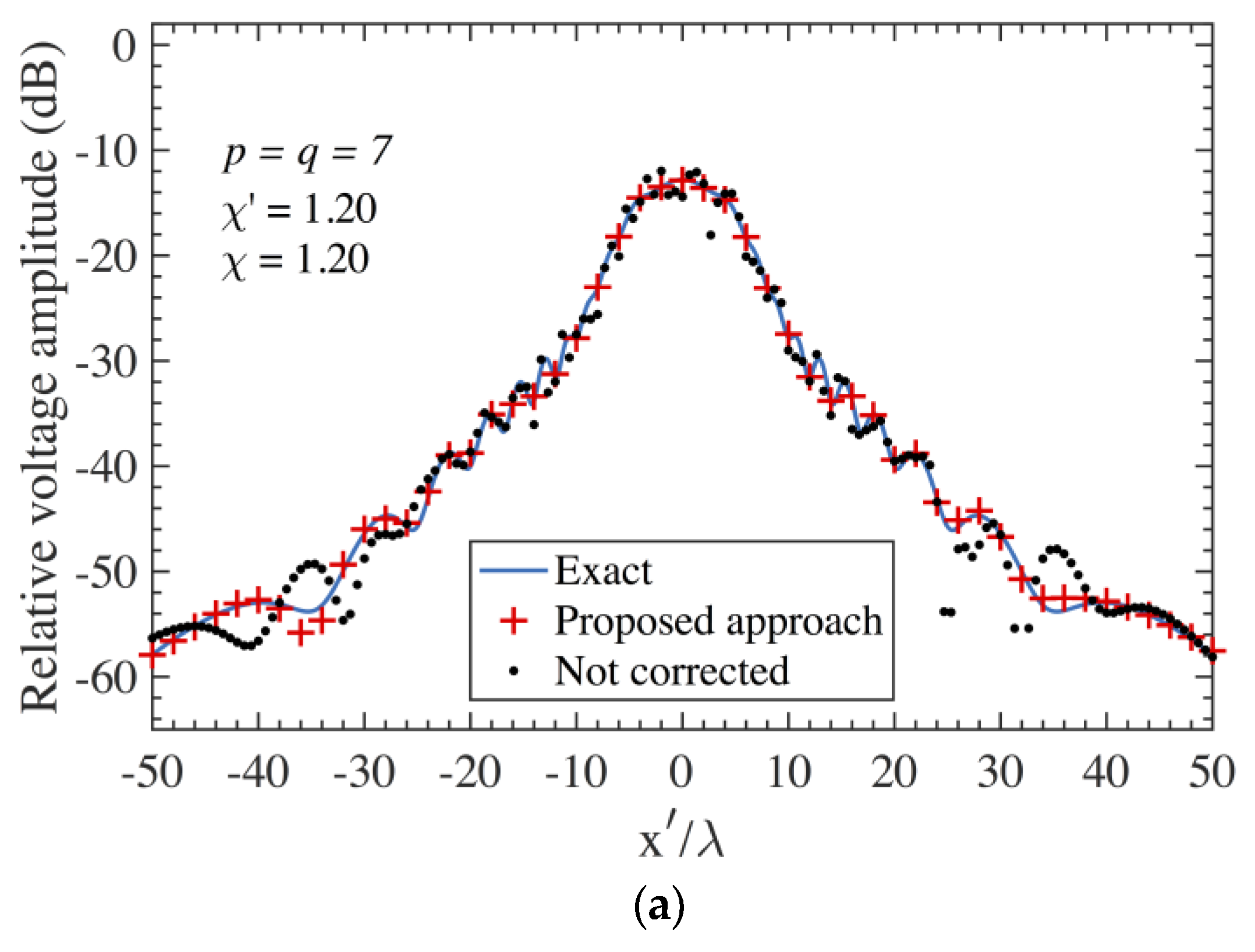
The effectiveness of the devised procedure is first assessed by the NF reconstructions. To this end, the exact amplitudes and phases of the voltages $V_y$ along the horizontal line of the scanning plane at y’ = 3λ are compared in Figure 3a,b for AUT 1 and in Figure 4a,b for AUT 2 with those recovered through the 2D OSI Formula (6) from the acquired PWMS data, after the positioning errors affecting them have been compensated by first employing the k-correction formalized in (13) and subsequently the iterative strategy. For sake of comparison, the reconstructions obtained by directly interpolating the PWSM samples corrupted by the considered 3D probe positioning errors through (6) are also shown in the same figures. Moreover, the analogous comparisons relevant to the AUT 1 on the scanning line at y’ = 15 λ are presented in Figure 5a,b, whilst those relevant to the AUT 2 on the scanning line at $y\prime$ = 13 λ are shown in Figure 6a,b. In all the reconstructions from the data affected by 3D positioning errors, the solution of the linear system involved in the iterative procedure has been obtained by choosing 10 iterations which are enough to ensure the convergence of the algorithm with very small errors [20]. It should be noted that, for both the AUTs, despite the simulated data affected by severe 3D positioning errors, the recoveries achieved by using the devised approach are shown to be very accurate, apart from some little disagreements occurring in the outer zone characterized by a very low voltage amplitude.

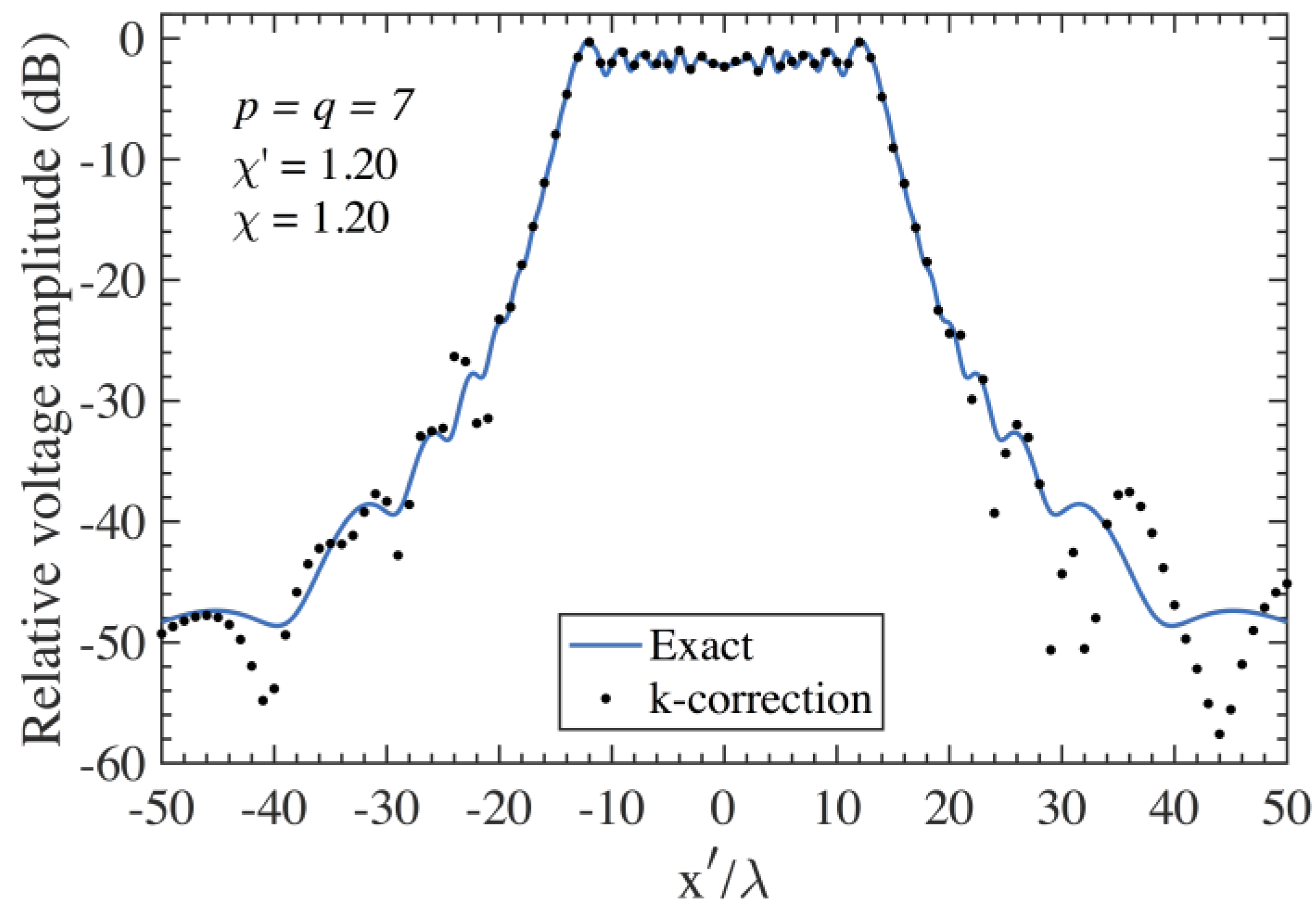
To show the need for using the proposed iterative procedure after applying the k-correction to compensate the deviation from the considered measurement plane, the reconstruction of the amplitude of the voltage $V_y$ along the line at $y\prime$= 3 λ is again reported in Figure 7 for the AUT 1 and Figure 8 for the AUT 2. These reconstructions have been obtained, in such a case, by adopting only the k-correction as performed in [17], without applying the iterative procedure. Accordingly, it results:

$$V(x\prime ,y\prime ,0)=V(x\prime +{\delta }_{\ell x},y\prime +{\delta }_{\ell }{}_y,{\delta }_{{\ell }_z}){\mathrm{e}}^{\mathrm{j}2\pi {\delta }_{{\ell }_z}/\lambda }$$

(19)

where $V(x\prime +{\delta }_{\ell x},y\prime +{\delta }_{\ell }{}_y,{\delta }_{\ell }{}_z)$ is the voltage corrupted by 3D positioning errors and $V(x\prime ,y\prime ,0)$ is the corrected one. Clearly, such an approach does not allow for a precise reconstruction, thus further assessing the effectiveness of the devised multi-steps compensation procedure.

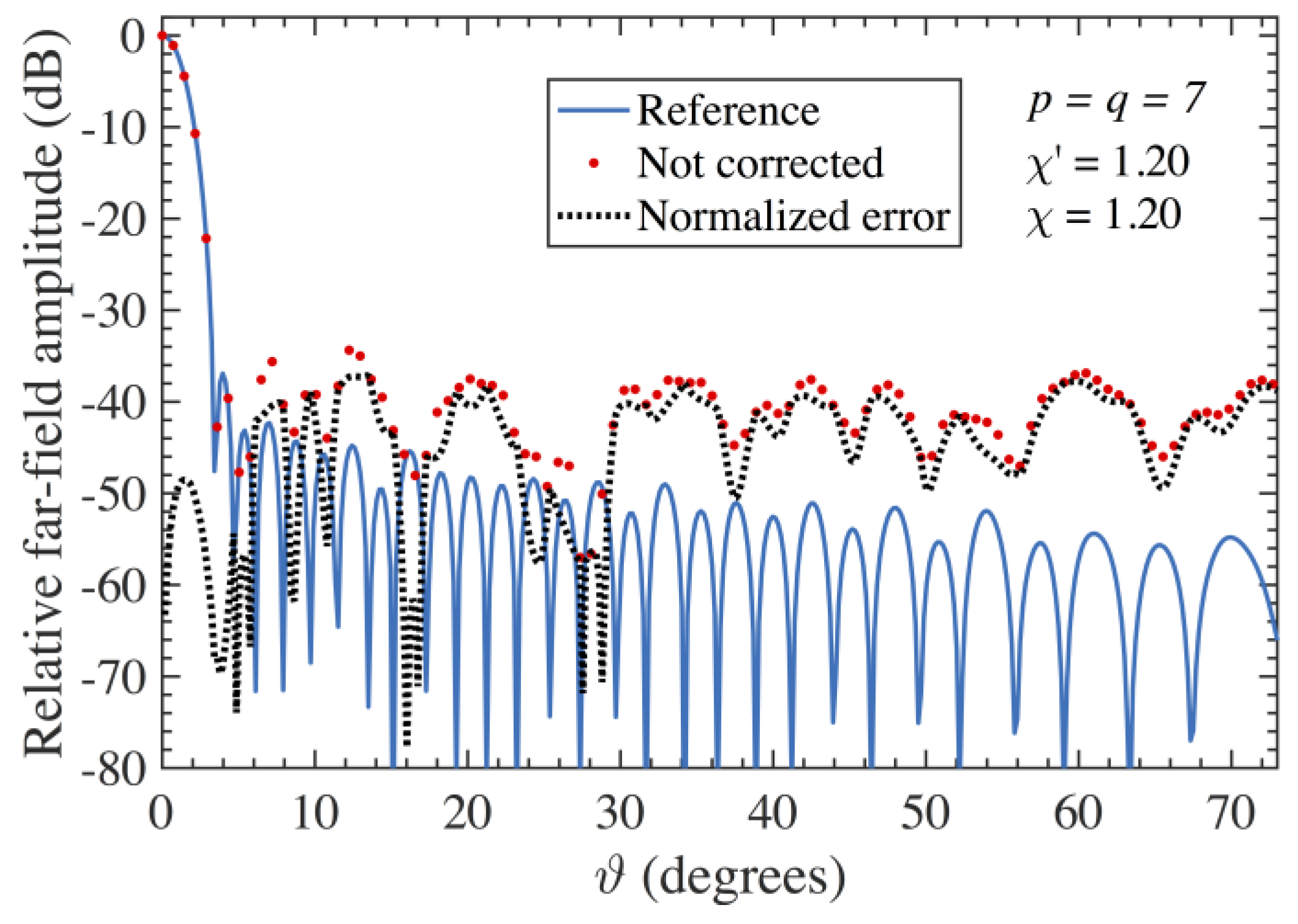
The overall effectiveness of the multi-steps compensation approach is assessed in the following by the reported FF reconstructions. Since the proposed AUTs show almost the same FF patterns in the principal planes, only the results relevant to the E-plane are here shown. Accordingly, the FF patterns obtained from the PWMS data after that the 3D probe-positioning errors have been corrected are compared in Figure 9 for the AUT 1 and Figure 10 for the AUT 2 with those (references) computed by using the exact PR samples. Furthermore, for comparative purpose, the E-plane FF patterns obtained when the proposed compensation approach is not applied are also shown in Figure 11 (AUT 1) and in Figure 12 (AUT 2). As can be clearly seen, in this case the reconstruction is shown to be extremely deteriorated, thus further validating the effectiveness of the devised errors compensation strategy. Such an effectiveness is even clearer from the very low errors presented in Figure 9 and Figure 10 as compared to the considerably greater ones reported in Figure 11 and Figure 12. Such errors have been evaluated by taking the differences between the references and recovered magnitudes, normalized to the maximum of the reference FF patterns and expressed in dB.

To conclude, it is interesting to compare the number of NF samples necessary to perform the PWMS and classic PR NF–FF transformations. The PWMS NF–FF transformation requires 8,649 samples for both the double bowl and the oblate spheroidal modellings, whilst the classic PR NF–FF transformation requires 40,401 samples. It is possible to achieve the same accuracy of the classic technique, but saving about 80% of required samples.

Other representative results relevant to the application of the devised procedure for correcting 3D positioning errors in the NF–FF transformation with PWMS based on the oblate spheroidal AUT modelling have been preliminarily presented in [30].

5. Conclusions

In this paper, effective NF–FF transformations for quasi-planar AUTs from 3D probe positioning errors corrupted PWMS data have been developed and numerically validated. To this end, a multi-steps compensation procedure has been properly devised. Such a procedure exploits, as a first step, the k-correction to compensate for the positioning errors occurring when the actual sampling points deviate from the considered scanning plane. After that, an iterative algorithm is used to restore the regularly distributed samples from those previously obtained and affected only by 2D positioning errors. Once the correct PWMS samples have been reconstructed, the huge NF data required to compute the standard PR NF–FF transformation are evaluated by using the 2D OSI formula.

Notwithstanding the severe 3D positioning errors corrupting the PWMS samples, the NF and FF reconstructions, obtained by employing the devised compensation approach, are very accurate, especially when compared to the severely deteriorated ones calculated without using this procedure. Thus, the effectiveness of the developed approach is thoroughly assessed.