1. Introduction
Networks are an abstract representation of complex systems throughout the sciences. Studying complex networks can reveal numerous potential associations between elements. Traditional network models represent individual elements as nodes and capture the relationships between elements through links connecting the nodes [
1,
2,
3]. In this way, the relationships between pairs of individuals can be represented as links in a social network, the functions of pairs of proteins can be abstracted as links in a protein network, and an email network can also serve as a representation of interactions among pairs of colleagues or other people [
4,
5,
6,
7]. However, the representation through pairs alone cannot adequately describe systems that involve higher-order interactions between more than two entities. We can observe several relevant examples. For instance, people often interact within social groups, associative relations among proteins frequently involve the function of multiple proteins, rather than just pairs, and people also frequently send group emails.
Link prediction is an important research topic in complex networks, which deals with the task of predicting the likelihood of two nodes in a graph being connected at some point in the future [
8,
9]. Predicting unknown links often relies on the known ones in the network. Traditional network models only describe the relationships between pairs of nodes. Therefore, some classic algorithms often extract only low-order features of the nodes from the network, such as the hub depressed index (HDI) [
10], Adamic-Adar [
11] based on common neighbors, and resource allocation indicators (RA) [
12], among others. In addition, graph embedding, which aims to learn the features of nodes, has emerged as an effective methodology for many downstream tasks, such as link prediction [
13,
14,
15,
16], community detection [
17,
18], etc. The fundamental concept of these algorithms is to acquire node sequences through random walks in the network and subsequently learn the embedding of each node using a skip-gram model [
19,
20]. This approach characterizes the higher-order structure features of nodes within the network. However, many previous works have employed connectivity or structural similarity as measures of node similarity, such as DeepWalk [
21], graph2vec [
22], and node2vec [
23]. Connectivity reflects the similarity between nodes in the network where links exist. For example, when two nodes have more common neighbors, it is highly likely that a link will exist between them. On the other hand, structural similarity measures whether two nodes have similar local structures in the global network. For instance, in a social network, if both managers of two departments are local hub nodes, it is more likely that a link will exist between them. Most known representation techniques only learn representations for nodes from the perspective of one kind of similarity. LEMON [
24] introduces motifs as supervertices in the network for random walks and captures the structural similarity of nodes by performing random walks to the supervertices. However, this approach introduces nine types of motifs, considering too many structural features in the second and third orders. This might lead to overfitting during the process of learning node embeddings. Additionally, having more motifs implies higher time complexity, making the model less suitable for application in large-scale networks. Meanwhile, this approach considering connectivity and structural similarity is based on traditional networks, which only can illustrate the relationship between pairs of nodes. A significant amount of information is discarded when a network is generated, such as group emails, student class, multiple proteins information, etc. Therefore, how to characterize higher-order interaction features of nodes in a network is a problem that we have to address.
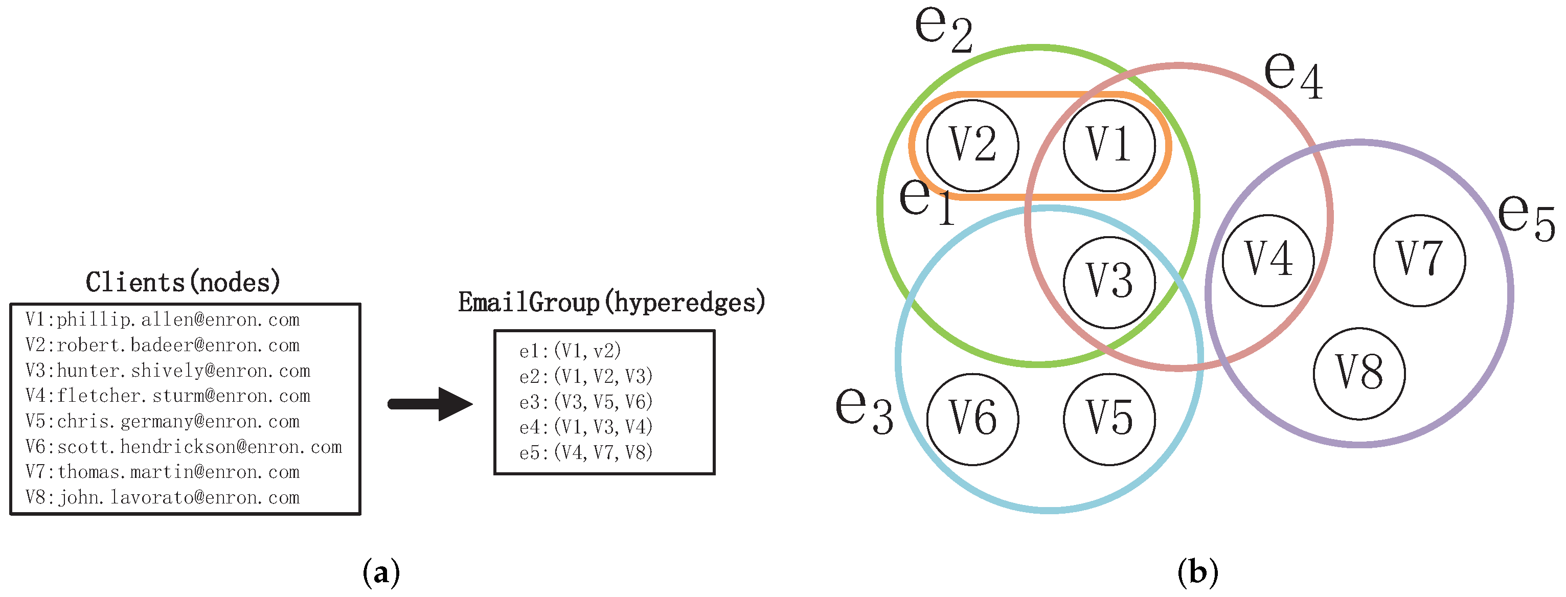
Hypergraphs [
25], which consist of nodes and hyperedges, can tackle the aforementioned problem. Each hyperedge has the capability to connect any number of nodes, representing higher-order interactions within groups of nodes [
26,
27,
28]. For instance, the interaction relationships shown in
Figure 1a are naturally represented by the hypergraph depicted in
Figure 1b Each hypergraph corresponds to an email. The nodes in the hypergraph represent the Enron employees who are senders or recipients of the email. The hypergraph
represents the interaction between
and
, while the hypergraph
describes the interaction among
,
, and
. This demonstrates that a hypergraph is capable of distinguishing pairwise relationships and higher-order interaction relationships. Additionally, the hyperedge
represents pairwise relationships, thus traditional “node–edge”-structured networks can be regarded as a special form of hypergraph.
In this paper addressing the issues of overfitting and excessively high time complexity in the LEMON method, we propose the Learning Embedding based on Clique Of the Network method (LECON), which utilizes Clique structures instead of motifs as supernodes to reconstruct the network. Then, the node sequences are input into the skip-gram model for learning node embedding vectors. Subsequently, addressing the limitation of traditional “node–edge”-structured networks in capturing group relationships, we present the HyperMotif Representation Learning on Hypergraph (HMRLH) method, which employs hypergraphs to model the network and incorporates hypermotifs as supernodes for assessing the structural similarity among nodes. Additionally, to acquire node sequences that more accurately capture node characteristics, we introduce a Depth and Breadth Motif Random Walk method. This method incorporates hyperparameters, designated as p and q, to regulate the walking patterns. We employ this walking technique independently with the LEMON and HMRLH methods to assess its efficacy.
The structure of this paper is organized as follows:
Section 1 elucidates the current state of affairs in both domestic and international contexts, along with the shortcomings of existing algorithms.
Section 2 introduces some of the prior work that is referenced in this paper; consequently,
Section 3 provides a detailed description of the structure of our proposed methods. In
Section 4, we conduct experiments to validate the effectiveness and feasibility of our proposed methods. Finally, we summarize and discuss all the work presented in this paper.
3. Approach
Firstly, we examined the influence of considering only two fully connected motifs (Cliques) on the algorithm’s experimental performance, utilizing the nine motifs introduced by LEMON. Subsequently, we introduce a novel representation learning method called HMRLH, which builds upon LEMON, to establish a relationship between connectivity and structural similarity using hypergraphs. Finally, we introduced a Depth and Breadth Motif Random Walk method to capture node sequences and applied it to both the LEMON and HMRLH methods.
3.1. LECON
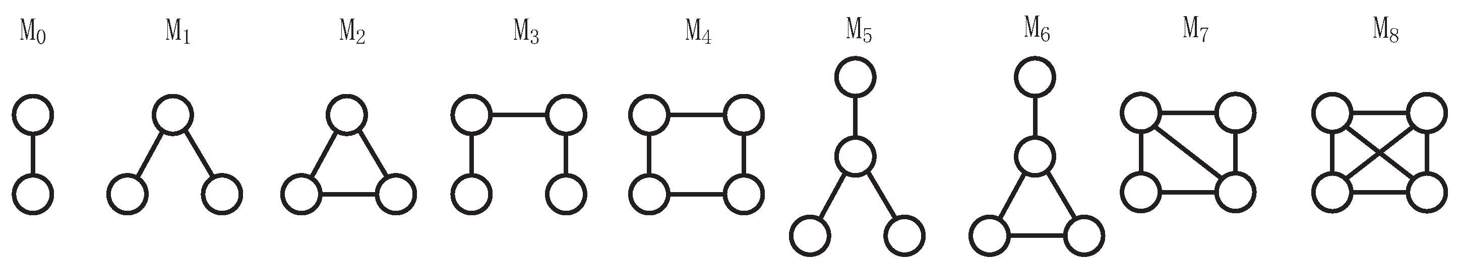
LEMON extracts the structural information of nodes through motifs. However, it introduces nine types of motifs, including second-order, third-order, and fourth-order motifs. More motifs imply higher time complexity, which may make it unsuitable for large-scale networks. Additionally, the use of multiple motifs in learning node features can potentially lead to overfitting.
Based on the aforementioned issues, we conducted a comparative study by considering only two fully connected motifs (Cliques) among the nine motifs introduced by LEMON. This modified approach is referred to as LECON (Learning Embedding based on Clique Of the Network).
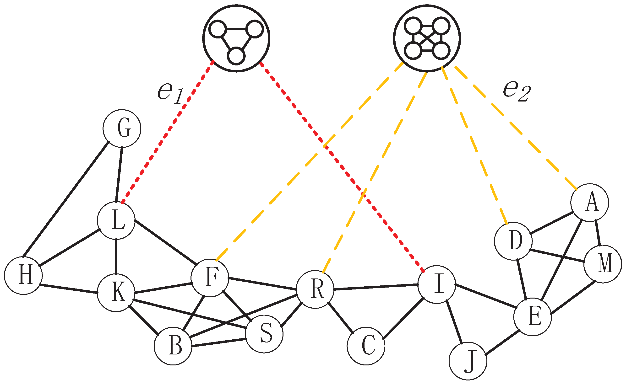
As shown in
Figure 5, LECON introduces only 2-Cliques and 3-Cliques as supernodes. If a node
v is part of these Cliques, a structural edge will be established between node
v and the respective Clique. In a "node–edge" network, node
L is connected to nodes
G,
H,
K, and
F, respectively. Upon observation, it becomes evident that nodes
L,
G, and
H form a 2-Clique, which leads to node
L generating a structural edge (
) with the 2-Clique supernode. Similarly, nodes
A,
D,
M, and
E constitute a 3-Clique, resulting in the generation of a structural edge (
) between node A and the 3-Clique supernode.
3.2. HMRLH
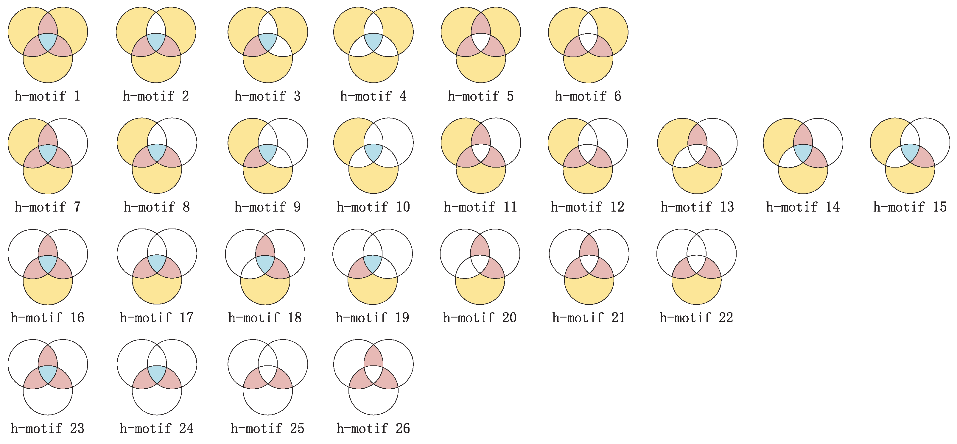
While the LEMON algorithm considers the motif structure of traditional "node–edge"-structured networks, it is important to note that "node–edge"-structured networks can only represent pairwise relationships between nodes. When higher-order interactions are present, "node–edge’-structured networks exhibit limited expressiveness. To enhance the expressiveness of the model, we propose using a hypergraph to model the network and introducing hypermotifs as supernodes. However, in the third order alone, there are 26 species of hypermotifs. Treating all of them as supernodes would significantly increase the model’s time complexity. Based on the findings in
Section 4.4.1, it can be concluded that when LECON considers only two fully connected motifs, there is minimal loss, and in some cases, even an improvement in modeling effectiveness, all while reducing time complexity. Thus, to address the challenge of high time complexity, we categorize the 26 hypermotifs into two types: open and closed hypermotifs.
In this study, we introduce mapped third-order hypermotifs as supernodes in the hypernetwork to construct the HMRLH (HyperMotif Representation Learning on Hypergraph) model. Using the third-order hypermotif as an example, we categorize it as a closed motif when these three hyperedges share one or more common nodes, or when there is a common node between every pair of the three hyperedges. On the contrary, if only one of the three hyperedges shares a common node with the other two hyperedges, we consider that these three hyperedges form an open motif.
As shown in
Figure 6, hyperedges
,
, and
share the common node
L, so we map them to a closed hypermotif. Furthermore, a structural edge will be generated between nodes that belong to these hyperedges and the closed hypermotif. Regarding hyperedges
,
, and
, hyperedge
shares one common node with the hyperedges
and
, respectively, while hyperedges
and
do not share a common node. This falls under the category of mapping to open hypermotifs, as we described.
Unlike LEMON, in the HMRLH model, the weights of structural edges between node
u and supernode
are denoted as
, as shown below:
where
indicates the number of the
i-th type of hypermotif containing hyperedges
.
As can be seen from
Figure 6, hyperedges
,
, and
construct a closed hypermotif; hence,
,
, and
are all equal to 1. For node
H, which only belongs to
,
is equal to 1. However, for node
L, which belongs to all hyperedges
,
, and
,
is equal to the sum of
,
, and
.
3.3. Depth and Breadth Motif Random Walk
For the motif-step random walk method used by LEMON, only whether the nodes are neighboring nodes or not is considered when the random walk is between nodes. Previous work, such as node2vec [
23], demonstrated that sequences obtained by considering both depth-first and breadth-first traversal are more reflective of the structural properties of the nodes during random walks. Therefore, inspired by node2vec, this work introduces parameters
p and
q to control the random walk between neighboring nodes based on motif-step random walk. Assuming starting from node
u, the formula for random walk is as follows:
where
c indicates the probability of walks traveling from a normal node to a supernode, while the probability of traveling on normal edges is equal to
. When traveling on normal edges, that is, when wandering to the first-order neighboring node in the network at the next step, the probability of going from node
v to
x is shown in the below formula. First, we consider that a random walk has occurred on edge
, and then we decide which node to walk to next based on the probability.
where
represents the distance between node
t and the next node
x. The parameter
p controls the likelihood of revisiting the previous node
t, which are two hyperparameters. If
p is set to a high value (>
(
q,1)), we are less likely to sample already visited nodes in the next step. The parameter
q controls our preference for walking with BFS or DFS. If
, the random walk is biased towards the first-order neighbors of node
t, approximating BFS. In this sense, our sampling focuses on nodes within a small local range. On the contrary, if
, the walk is more likely to visit second-order neighbors of node
t in relation to node
v.
3.4. LECON-DB and HMRLH-DB
In order to verify the effectiveness of our proposed Depth and Breadth Motif Random Walk method, we incorporated it into the LEMON and HMRLH methods for experimental validation. These modified methods are referred to as LEMON-DB and HMRLH-DB, respectively.
4. Result
4.1. Datasets
Since the method proposed in this paper places more emphasis on the higher-order structure within the network, we chose networks with varying densities for separate comparative experiments. We utilized the following datasets for conducting our experiments:
Email-Enron [
34]: Each hyperedge corresponds to an email, with the nodes within the hyperedge representing Enron employees who either sent or received the email. The dataset was downloaded from
https://snap.stanford.edu/data/email-Enron.html (accessed on 27 May 2023).
TCM: This dataset comprises 100 ancient classical prescriptions provided by the State Administration of Traditional Chinese Medicine (SATCM) in China.
TFD: The dataset consists of formulas contained in the classical Chinese medical text “Treatise on Febrile Diseases”.
SPGC: This dataset is sourced from the first 25 volumes of the classical Chinese medical text “Synopsis of Prescriptions of the Golden Chamber”.
Among them, the TCM, TFD, and SPGC datasets were constructed by our team members who collected and organized relevant documents.
As shown in
Table 1, we present some statistics of the datasets.
It can be observed that the Email-Enron dataset comprises 143 nodes, 2585 edges, 1542 hyperedges, and an average degree of 36.13. These statistics underscore the higher network density and the more pronounced higher-order structure within the Email-Enron dataset. In contrast, we utilize a TCM dataset characterized by a greater number of nodes, fewer edges, half the average degree of the Email-Enron dataset, relatively low network density, and fewer higher-order features. In addition, to further investigate the impact of the network’s higher-order structure on algorithm performance, we introduced the TFD and SPGC datasets. Compared with the TCM dataset, these two datasets increase the network’s average node degree by adding more nodes and edges, respectively, resulting in denser networks with more prominent higher-order features.
4.2. Evaluation Metrics
This paper evaluates the performance of the algorithm using the area under the ROC curve (AUC) and precision. The AUC is employed to assess the overall performance of the algorithm, whereas precision is focused on evaluating the accuracy of the top-ranked edges in the prediction results.
4.3. Experimental Environment
The experiments in this paper were conducted on a Windows 10 operating system with 16 GB of RAM and an i7-7600U 2.90 GHz CPU. The programming language used was Python, version 3.8.8. The construction of the adjacency matrix was implemented using NumPy, version 1.19.5, and the traditional network was built using NetworkX, version 2.3.
4.4. Experimental Results
In order to better validate the performance of the method proposed in this paper, we conducted five sets of comparison experiments with other related algorithms on each of the four datasets mentioned above. We utilize cosine similarity to measure the similarity between nodes and rank the predicted edges by score.
4.4.1. LECON and LEMON
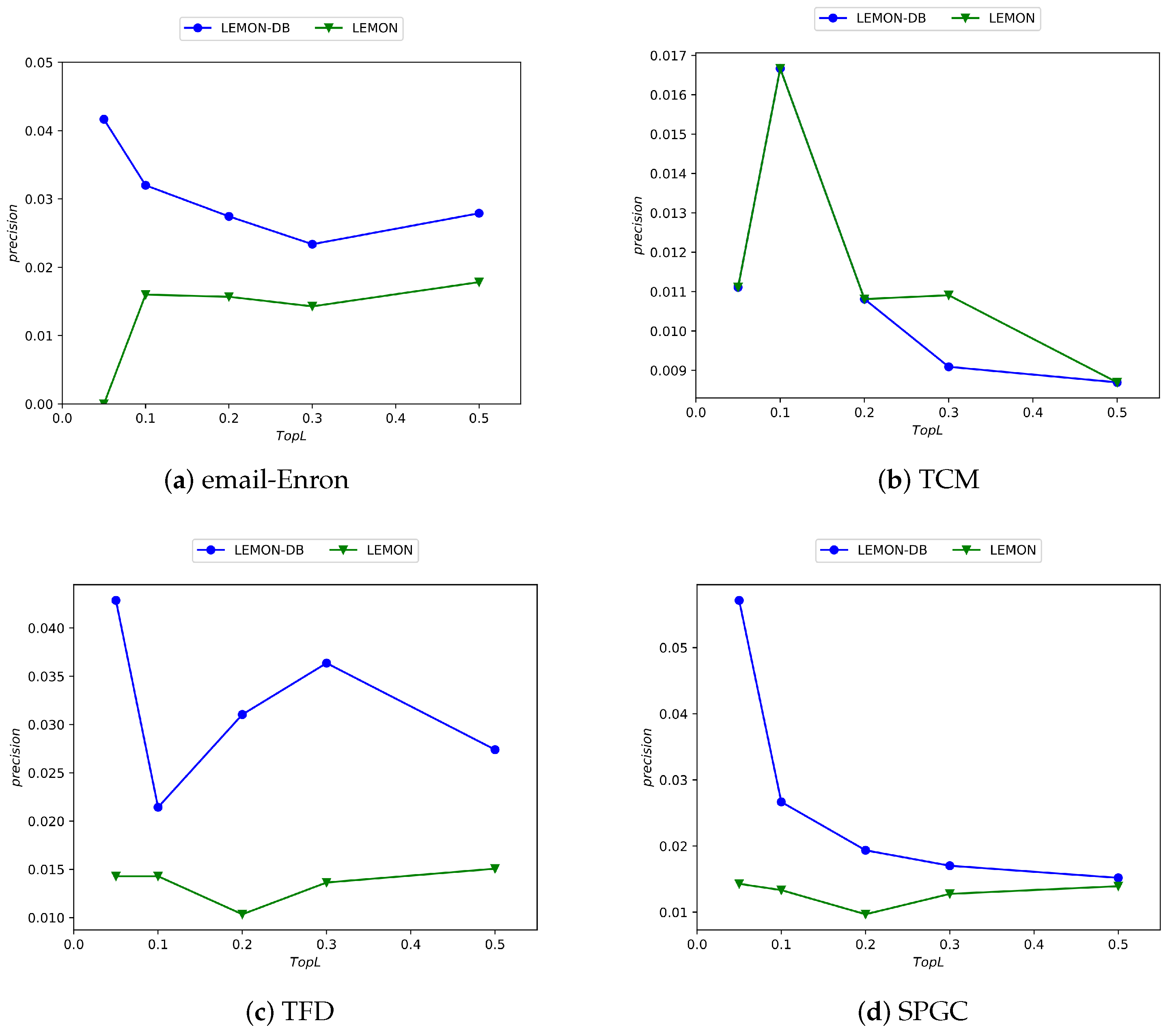
LEMON incorporates nine types of 3-motifs as supernodes. To address time complexity concerns, we propose the LECON algorithm, which focuses solely on two of these fully connected structures derived from LEMON. Below, we can observe the performance of both algorithms across four distinct datasets.
As depicted in
Figure 7, the horizontal axis corresponds to the percentage of top-
L-ranked edges by precision score, while the vertical axis indicates the precision value. It is evident from the figure that the LECON algorithm exhibits improved performance across nearly all datasets compared with the LEMON algorithm, despite the reduction in time complexity.
4.4.2. LEMON-DB and LEMON
To validate the effectiveness of the Depth and Breadth Motif Random Walk method, we incorporated it into the LEMON algorithm and conducted comparative experiments. The experimental results are as follows.
Figure 8 clearly illustrates that the performance of the LEMON-DB method, following the incorporation of the Depth and Breadth Motif Random Walk, surpasses that of the original LEMON algorithm. This demonstrates that the Depth and Breadth Motif Random Walk method effectively captures the network node features.
4.4.3. HMRLH and LEMON
In this section, to validate the effectiveness of hypergraph modeling in characterizing node features, we compare the HMRLH method using hypergraphs and hypermotifs with the LEMON method. The experimental results are presented
Figure 9:
From the experimental results, it can be concluded that the HMRLH method, which incorporates hypergraph and h-motif modeling, outperforms the LEMON algorithm on the datasets used in this paper. This further underscores the advantages of hypergraph modeling in capturing higher-order interaction structures compared with traditional network structures.
4.4.4. HMRLH-DB and HMRLH
Similarly, to further validate the performance of the Depth and Breadth Motif Random Walk method, we introduced it into HMRLH, resulting in the HMRLH-DB approach. Below are the comparative experimental results between HMRLH-DB and HMRLH.
From
Figure 10, it can be observed that only in the Email-Enron dataset is the performance of the HMRLH-DB method slightly inferior to that of HMRLH. However, in the other three datasets, the HMRLH-DB method outperforms HMRLH. This further demonstrates the effectiveness and feasibility of the Depth and Breadth Motif Random Walk method.
4.4.5. Comparison with Baselines
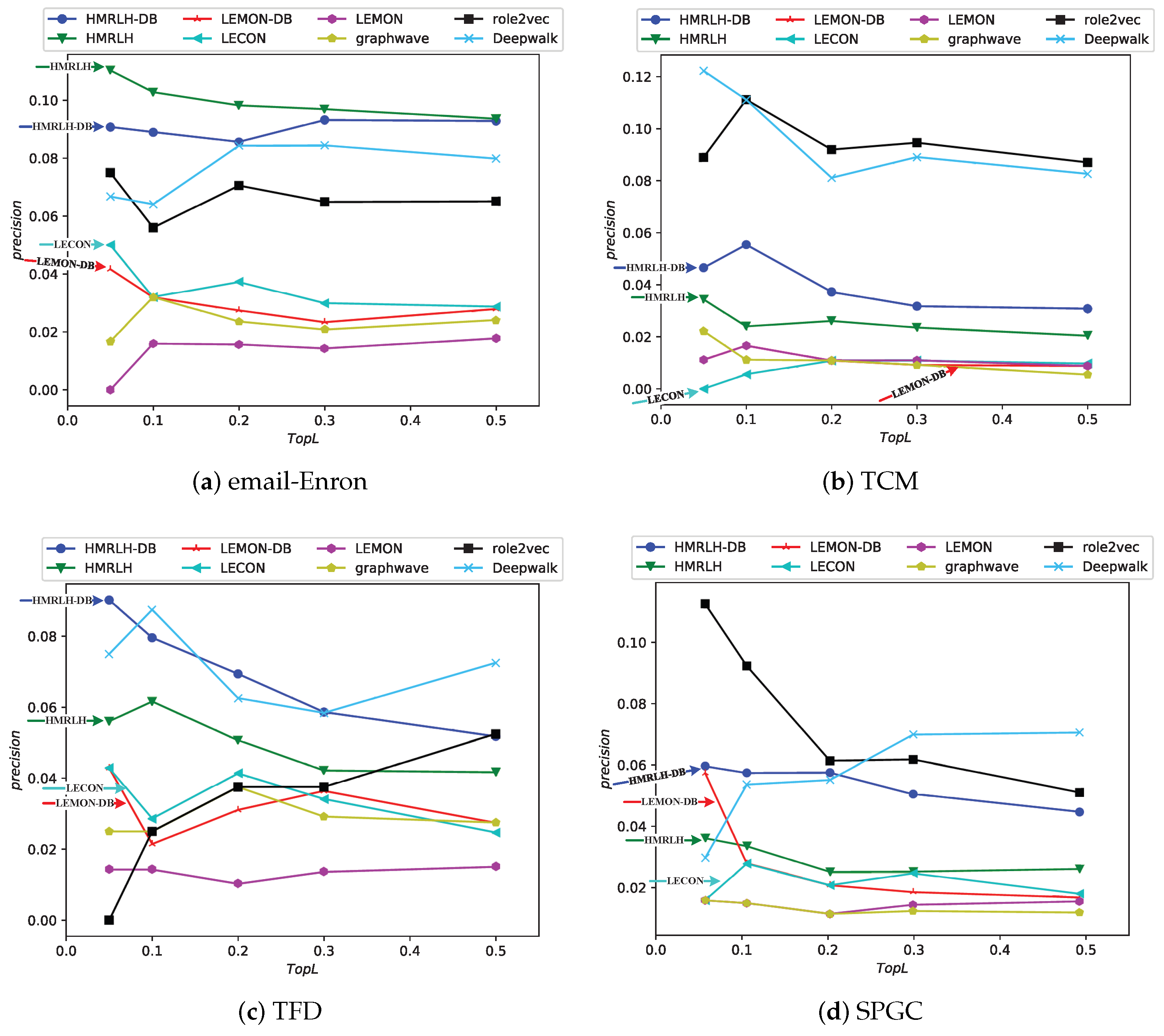
In this section, we use the four proposed methods to compare them with the following baselines.
LEMON [
24]: The LEMON method, which constructs a network by introducing nine types of motifs as supernodes and then learns node features through random walks, serves as the primary reference approach in our work.
DeepWalk [
21]: Deepwalk extends recent developments in language modeling and unsupervised feature learning, originally applied to word sequences, to the domain of graphs. It leverages local information extracted from truncated random walks, treating these walks as analogous to sentences, to acquire latent representations.
Graphwave [
35]: GraphWave is an approach that captures the network neighborhood of each node through a low-dimensional embedding, utilizing heat wavelet diffusion patterns.
Role2vec [
36]: Role2Vec framework employs the versatile concept of attributed random walks, providing a foundation for extending current techniques like DeepWalk, node2vec, and numerous others that make use of random walks.
The experimental results are depicted in the
Figure 11:
From the experimental results, it can be observed that in the Email-Enron and TFD datasets, the performance of the proposed HMRLH and its related algorithms is superior to the compared baselines. In the SPGC dataset, its performance is slightly inferior to that of Role2Vec. However, the performance in the TCM dataset is not as promising, which may be attributed to the fact that the HMRLH algorithm proposed in this paper primarily focuses on learning node features by considering higher-order structural information within the network. As indicated by the previous analysis, the TCM dataset lacks prominent higher-order structural characteristics. Consequently, the HMRLH algorithm does not outperform other methods when it comes to learning node features on the TCM dataset.
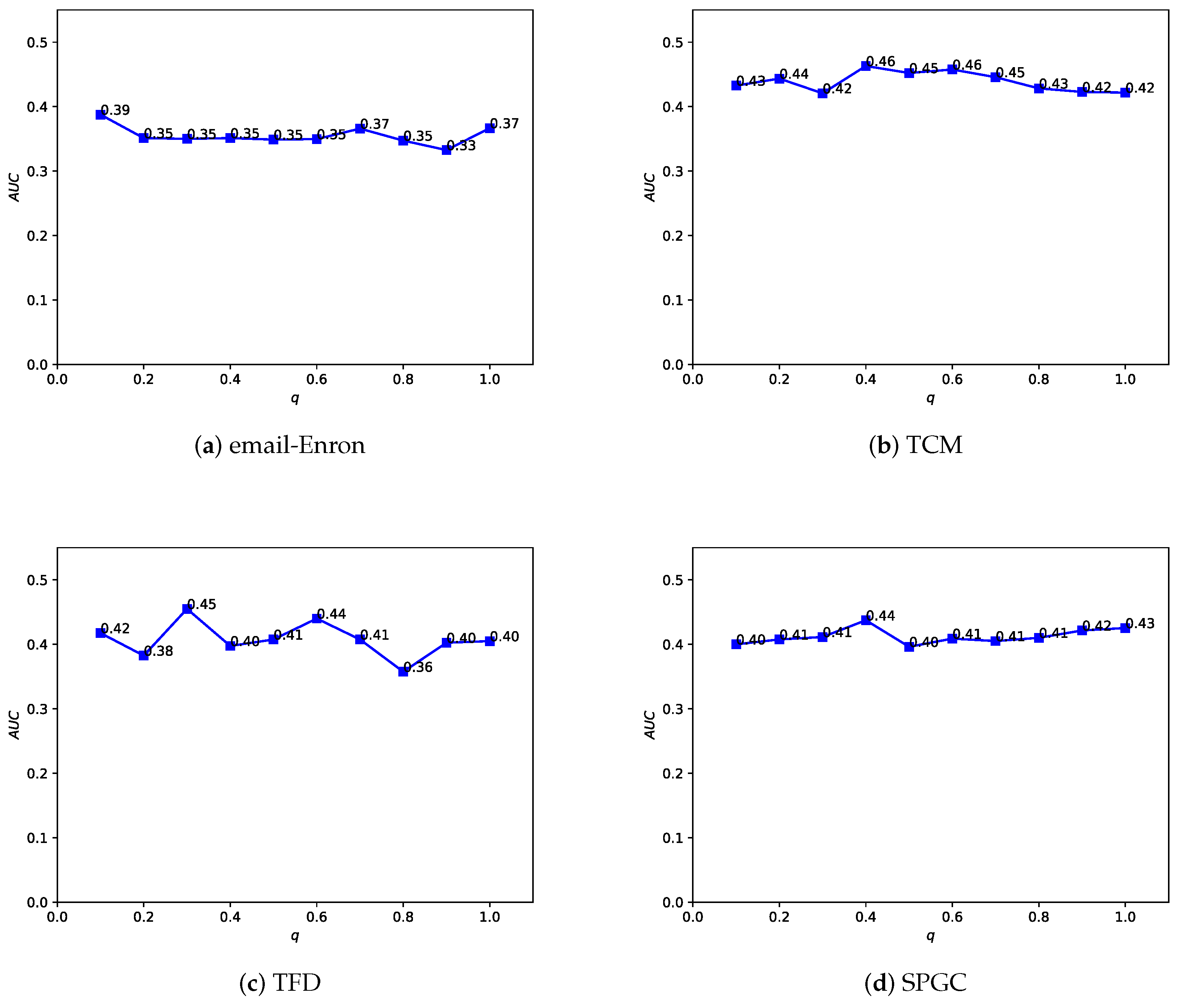
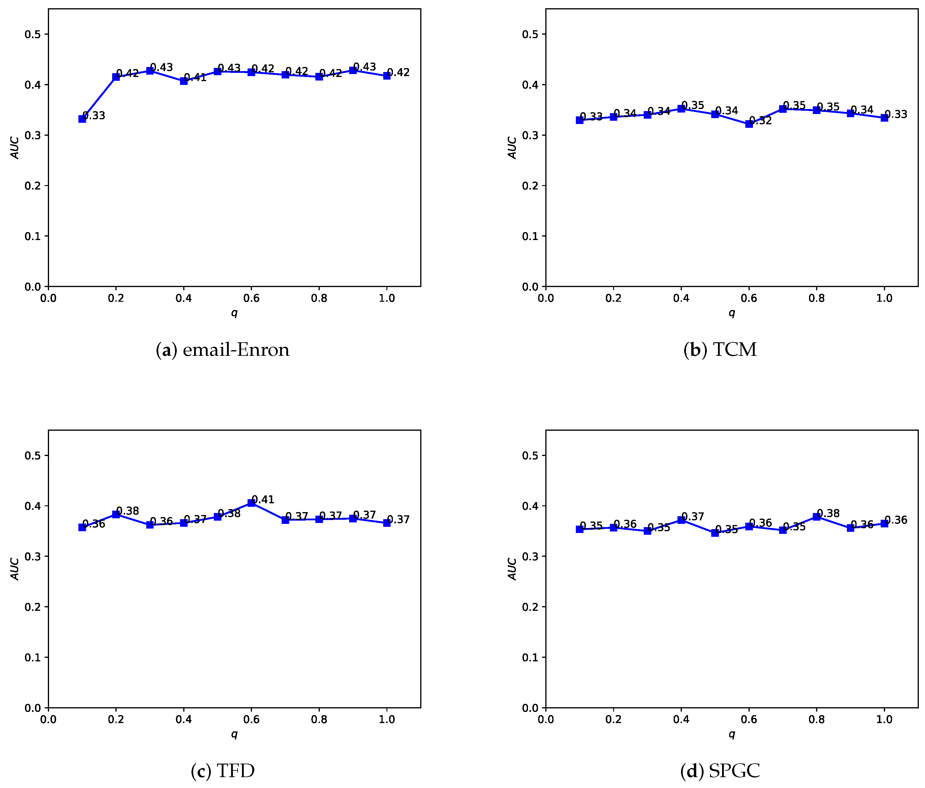
4.5. Parameter Sensitivity
In the Depth and Breadth Motif Random Walk method, we introduced two hyperparameters,
p and
q. Among them, parameter
p is used to control the probability of returning to the previous node. Following the original paper, we set
. Parameter
q is used to control whether the random walk on the regular network leans more toward BFS (Breadth-First Search) or DFS (Depth-First Search). The difference between the two lies in the fact that BFS tends to emphasize learning the structural similarity of nodes in the network, while DFS, on the other hand, places more emphasis on reflecting node connectivity during traversal. In the HMRLH method, we already represented the structural similarity of nodes in the network by introducing supernodes. Therefore, during the random walk process, we tend to focus more on learning the connectivity of nodes. Taking
, we conducted a sensitivity analysis on
q values within the range of 0 to 1, as shown in
Figure 12 and
Figure 13. As the
q value varies, the algorithm’s performance also undergoes changes. Analyzing the experimental results, it can be concluded that the algorithm performs relatively well when
q is set to 0.4 or 0.6.
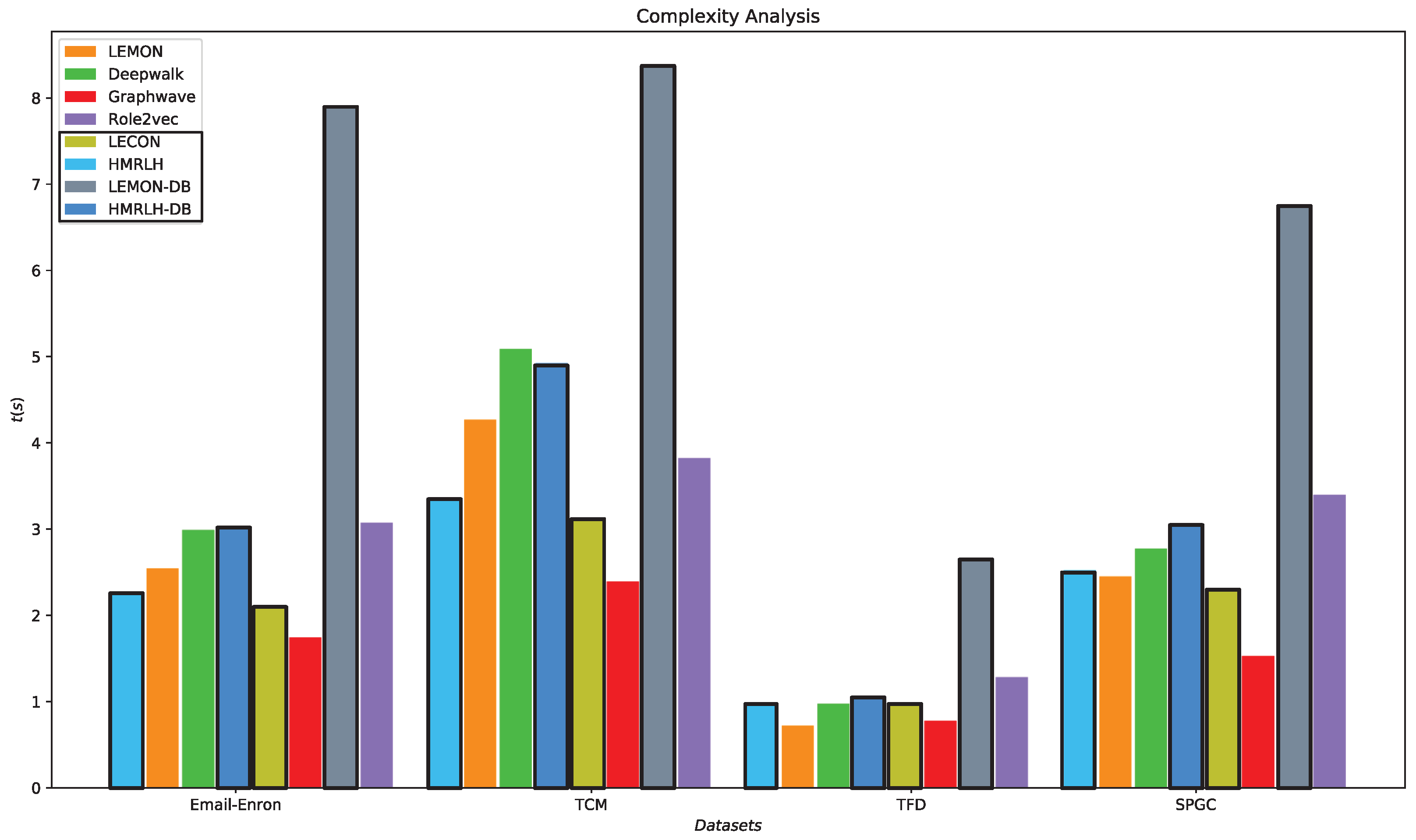
4.6. Time Complexity Analysis
The HMRLH method consists of two steps. First, it extracts hypermotifs from the network and reconstructs the network using these hypermotifs as supernodes. Then, it utilizes Depth and Breadth Motif Random Walk to obtain node sequences and learn node embeddings. The algorithm for extracting hypermotifs from the network is as follows (Algorithm 1):
| Algorithm 1:
Closed and Opened Hypermotif Count
|
Input: hypergraph: G = (V, E) Output: the number of open hypermotifs and closed hypermotifs corresponding to each node for
in E: for , in if != : if == : for in V: for in E: if in : return
end |
G represents the input network, and V and E represent the sets of nodes and edges, respectively. denotes the number of closed hypermotifs formed by hyperedge , and denotes the number of open hypermotifs formed by hyperedge . represents the number of closed hypermotifs formed by hyperedges containing node , and represents the number of open hypermotifs formed by hyperedges containing node .
Analyzing Algorithm 1, we can see that the time complexity for extracting hypermotifs is
, where
represents the number of hyperedges, L represents the average length of adjacency vectors, and
represents the number of nodes in the network. In the embedding phase, Depth and Breadth Motif Random Walk introduces two additional parameters,
p and
q, for calculating the probabilities of moving to each neighboring node when selecting the next walking node. Its time complexity is
, where
represents the number of nodes,
n represents the number of random walks, and
l represents the length of random walks. The runtime of each algorithm in the embedding phase on various datasets is illustrated in
Figure 14.
From
Figure 14, it can be observed that the runtime of the HMRLH method is generally slightly lower than that of the LEMON method. This is likely because the HMRLH method introduces only two types of supernodes, resulting in a relatively smaller selection when generating random walk sequences. On the other hand, algorithms LEMON-DB and HMRLH-DB, which incorporate the Depth and Breadth Motif Random Walk method, have relatively longer runtimes. This is primarily due to the higher time complexity of the Depth and Breadth Motif Random Walk method, which requires more time to generate walk sequences. However, in terms of algorithmic complexity, the HMRLH method, which incorporates hypergraph modeling, exhibits relatively lower time complexity compared with all the baselines.


