Towards Smarter Positioning through Analyzing Raw GNSS and Multi-Sensor Data from Android Devices: A Dataset and an Open-Source Application

Antoine Grenier; Elena Simona Lohan; Aleksandr Ometov; Jari Nurmi

doi:10.3390/electronics12234781

,

and

Electrical Engineering Unit, Tampere University, 33720 Tampere, Finland

^*

Author to whom correspondence should be addressed.

Electronics2023, 12(23), 4781;https://doi.org/10.3390/electronics12234781

This article belongs to the Special Issue Wearable Sensing Devices and Technology

Version Notes

Order Reprints

Review Reports

Abstract

The state-of-the-art Android environment, available on a major market share of smartphones, provides an open playground for sensor data gathering. Moreover, the rise in new types of devices (e.g., wearables/smartwatches) is further extending the market opportunities with a variety of new sensor types. The existing implementations of biometric/medical sensors can allow the general public to directly access their health measurements, such as Electrocardiogram (ECG) or Oxygen Saturation (SpO2). This access greatly increases the possible applications of these devices with the combination of all the onboard sensors that are broadly in use nowadays. In this study, we look beyond the current state of the art into the positioning capacities of Android smart devices and wearables, with a focus on raw Global Navigation Satellite Systems (GNSS) measurements that are still mostly lacking in the research world. We develop a novel open-source Android application working in both smartphone and smartwatch environments for multi-sensor measurement data logging that also includes GNSS, an Inertial Navigation System (INS) magnetometer, and a barometer. Four smartphones and one smartwatch are used to perform surveys in different scenarios. The extraction of GNSS raw data from a wearable device has not been reported yet in the literature and no open-source app has existed so far for extracting GNSS data from wearables. Not only the developed app but also the results of these measurement surveys are provided as an open-access dataset. We start by defining our methodology and the acquisition protocol, and we dive into the structure of the dataset files. We also propose a first analysis of the data logged and evaluate the data according to several performance metrics. A discussion reviewing the capacities of smart devices for advanced positioning is proposed, as well as the current open challenges.

Keywords:

Global Navigation Satellite System (GNSS); Global Positioning System (GPS); low-power electronics; smart devices; smartphone; wearables; measurements; Android

1. Introduction

Interest in using smartphones for sensor logging has been part of the research community for the last decade. Smartphones provide a very interesting environment for data gathering, as they include a variety of sensors (e.g., accelerometers, gyroscopes, camera, Wireless Fidelity (WiFi), Bluetooth Low Energy (BLE)) embedded inside a low-cost platform. The Application Programming Interface (API) centralizes access to all the sensor measurements for Android devices, greatly simplifying the developments. Moreover, synchronization of all data is ensured by a common platform, making it useful for sensor fusion studies [1,2].

More recently, the development of “wearables” provides similar but new data-gathering platforms. On top of providing ultra-compact designs for the same sensors available on smartphones, smartwatches propose new kinds of sensors more related to health monitoring, such as ECG, photoplethysmogram (PPG), Galvanic Sensor Response (GSR), and/or SpO2. The different sensors in Android smart devices are displayed in Figure 1, showing the potential of smartwatches. While some manufacturers still propose their ecosystem (e.g., “ConnectIQ” for Garmin [3], Fitbit OS for Fitbit [4]), many manufacturers (e.g., Samsung, Google) are aligning on a common Android-based operating system with the possibility of common development of Android application on both the wearable and the smartphone platforms. This research will refer to them under the terms “smart devices”.

Figure 1. Sensors available in smart devices.

In the context of satellite positioning, all smart devices today include a GNSS receiver, yet the collection of measurements used to be limited to the device coordinates only. In 2016, Google enabled access to the “raw GNSS measurements” directly through the Android API. By “raw GNSS measurements”, we understand the measurements made by a receiver to compute a position, such as pseudoranges, carrier phases, Doppler shifts and Signal-to-Noise Ratio (SNR). Since the raw GNSS measurements were made available for smartphone manufacturers, the GNSS research community has been highly interested in the potential of enabling advanced high-precision positioning techniques on such devices, and many research works have been published to assess the receivers’ quality for positioning (see Section 2). We note that, as of today, Apple still needs to open access to the raw GNSS measurements in their OS, preventing similar comparisons on Apple devices. Thus, in this paper, we focus only on Android devices.

In the early years of Android GNSS measurements, only a certain number of Android models would provide access to raw data. Since Android 10 (API 29), Google made it mandatory for any Android device to support access to raw GNSS measurements. Discrepancies between device measurements are still present, but access to raw measurements is now open to potentially any Android devices and not only smartphones, including smartwatches.

The main contributions of this paper are as follows:

Developing a novel open-source sensor logging app called “Mimir”, designed for both smartphone and smartwatch environments;
Providing an open-source multi-sensor dataset acquired on various Android smart devices (four smartphones and one smartwatch), along with a geodesic-grade reference receiver;
Comparing the data quality and positioning accuracy of the Android smart devices in the context of positioning applications.

To the best of the authors’ knowledge, raw GNSS measurements acquisition comparison for smartwatch devices is conducted for the first time in the literature.

This research is performed in the context of the EU-funded projects APROPOS [5] and LEDSOL [6] that aim, among others, to also review low-power/low-cost devices, such as Android smart devices, for navigation purposes. The data acquired consist of four surveys, one static and three pedestrian/dynamic cases, and it was acquired in open-sky and urban areas. The complete dataset is released as an open source under a Creative Commons license CC-BY-4.0 on a Zenodo repository [7].

3. Methodology

In this section, we present the methodology for filtering the different Android devices, in order to select only a subset fitting our research. We proceed with detailing the different software used and developed to acquire and analyze the data, and we finish by presenting our survey protocol.

First, we recall some terminology used in this paper:

By “survey”, we mean the act of surveying and gathering data using a measurement device, as defined in land surveying topics.
In Differential GNSS (DGNSS), the “base” refer to the static receiver and “rover” refer to the moving receiver.
In GNSS, an “epoch” is defined a measure of time when a new GNSS measurement is received. A 1 Hz sampling rate would be equivalent to 1 epoch per second.

3.1. Device Selection

Research in Android GNSS measurements have shown that the measurement’s quality is not equal among all devices, even under identical measurement scenarios, as the manufacturers can embed different GNSS receivers in each new model [12]. Even access to specific GNSS observables (e.g., carrier phase, navigation message) cannot be ensured for each device. While the impact of these discrepancies can be minimal or unseen by the general user, it can prevent some of the research potential. Therefore, we performed the surveys over multiple Android devices for better assessment of their capacities in this study.

As the number of existing Android smartphones is enormous, the selection of the best devices can prove challenging. Thanks to the research community, a comprehensive list of Android devices with their GNSS capacities has been created through crowdsourcing and it is available online [32]. While it may contain multiple entries and some contradictory information, it still offers a first filter to select the devices with the required GNSS capacities. We note, however, that no smartwatch has been reported in this list so far.

To maximize the potential of each evaluated device and the quality of the dataset, we have decided to select devices under four constraints: (1) support of dual-frequency reception; (2) available carrier-phase measurements; (3) available navigation message; (4) GNSS chipset diversity. Point (3) was the most constraining, as many devices do not retrieve the satellite’s ephemeris from the navigation message anymore. Using the aforementioned list, we came down to only 22 devices checking all four requirements. More than half of them used a Broadcom BCM4775 or BCM4776 chip. The BCM4775 has been extensively reviewed in research before given that it was implemented in the Xiaomi Mi8 [10,14,17]; we have decided to focus on evaluating only the new generation BCM4776 instead. The rest of the receivers were chosen based on prices and in order to maximize GNSS chipset and manufacturer diversity. As one smartphone (Samsung A52) was already present in our lab for previous research purposes, we decided to also include it in these surveys for comparison purposes, even though it did not fit the requirements mentioned before. In total, four smartphones were selected and are summarized in Table 1. Note that while the Xiaomi 11T was said to have the navigation message enabled in the online list, we did not receive any during our experiments, and reported it accordingly in the table.

Table 1. Selected Android devices included in the dataset.

As no previous studies have looked into GNSS measurements in smartwatches, we decided to review the recently released Google Pixel Watch (October 2022) [33]. The watch also embeds a BCM4776 GNSS chip, similar to the one in the Pixel 7, enabling the measurement comparisons between both platforms. For example, while the BCM4776 is supposed to be dual-frequency-enabled, only L1 frequencies were received during the survey. The most logical hypothesis is that the dual-frequency reception was disabled in order to save energy, as it was proven to have a large impact on the energy budget of Android devices [34]. This shows that even when the GNSS chipset model is similar in two devices, large differences in the measurements can still be present.

In the following sections, devices will be referred to by the acronym listed in Table 1 for simplicity.

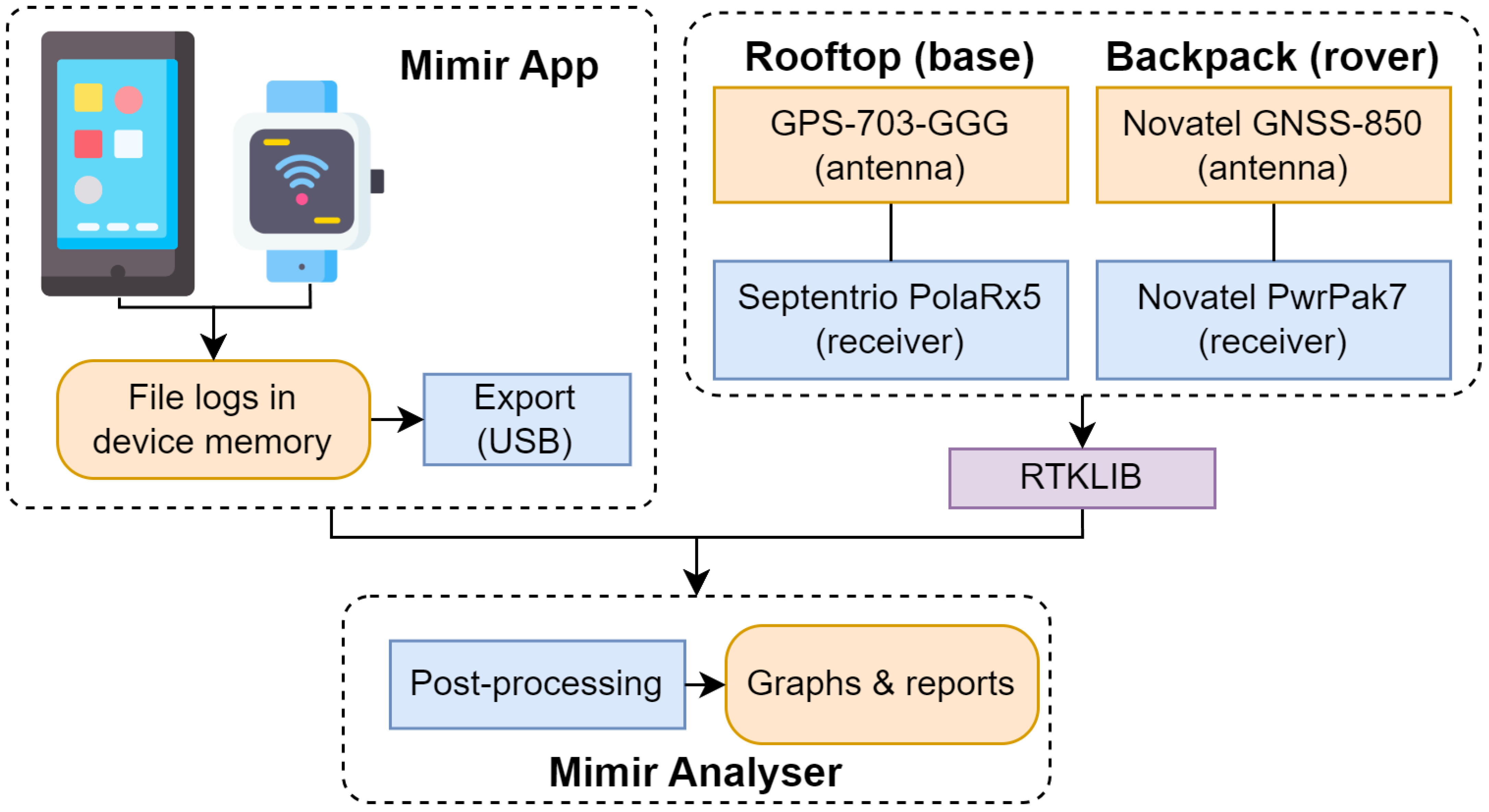
3.2. Logging Application Developments

In order to log the measurements inside the Android device, an app is used to interact with the Android API. Several apps exist today to log GNSS or sensor data, as reviewed in [11]. The most common one is GNSS logger [35], maintained by Google. It can log GNSS data in multiple formats (e.g., CSV, RINEX, NMEA). Logging other motion sensors is also possible, such as accelerometers, gyroscopes and magnetometers. However, several limitations of the existing applications were found during the first stages of our research. Firstly, only a partial version of the GNSSLogger source code is available on GitHub (old versions of the app), which prevents easy forking to the current version. Secondly, the logging is limited to GNSS and motion sensors logging only (no barometer data), with no possibility of controlling the sampling frequency. Thirdly, GNSSLogger does not exist for smartwatches, and, to the best of the authors’ knowledge, there is currently no app available for logging GNSS data from smartwatches.

Consequently, we decided to develop our own Android app called “Mimir”, a name based on the God of Knowledge in Nordic mythology (see https://www.britannica.com/topic/Mimir (accessed on 21 November 2023)). Mimir was developed with the goal of enabling the logging of any sensors present in an Android device. The code is released as open-source, under the Apache 2.0 license and is available on Github [36]. As mentioned earlier, while the Android smartwatch implements different flavors of the WearOS, they are based on a common Android API. Thus, the development of smartwatch apps is similar to smartphones, except for the UI design of the app. It allows the development of a common Android library for sensor logging, implemented in two different apps, for smartphones and smartwatches, respectively. Currently, the app allows logging of GNSS, motion and environment sensors, as defined in the Android developer documentation. The raw data are logged in a Comma Separated Value (CSV) format, similar to GNSSLogger logging format. For compatibility with the former processing software, all measurements related to GNSS have kept the same columns as in GNSSLogger. Other sensors are logged using our own defined format (see Appendix A). Furthermore, the app also allows the logging of health data on the smartwatch version. However, the recording of health data has been tested with the Google Pixel Watch only and is not recorded in the dataset provided for ethical reasons. Future developments planned are discussed in Section 7.

Note that similarly to GNSSLogger, no processing of the sensor is performed in the app. It is only used for sensor data gathering, logging the measurements exactly as provided by the Android API. Any post-processing is left to the computer processing software.

3.3. Analysis Software Developments

Once the data have been logged, it needs to be processed in order to analyze and use the sensor’s measurements for specific target applications; in our case, the target applications are based on accurate and/or robust positioning. The aforementioned GNSSLogger app is widely used by the research community because of its companion processing software called “GNSS Analysis App” [35], allowing plotting of the logged data. It is developed in Matlab and the source code can be found on GitHub. During the processing of the data, multiple unknown errors arose that prevented its usage for our analysis goals. Thus, similarly to how we developed the Mimir app [36], we have decided to build our own software to process the measurements.

For processing the data, we developed a Python library called “MimirAnalyzer”, with its code also available in open source on Github [37]. The library allows parsing of the CSV data into a Pandas DataFrame format, to be later analyzed. For a quick review of the measurement quality, we also created a local web dashboard. It allows visualization of the trajectory, comparison with a reference and review of the measurements logged into the file. For a deeper analysis, we have created also some Jupyter Notebook templates that allow for visuals and statistical analysis. More details about the performance metrics are provided in Section 5.

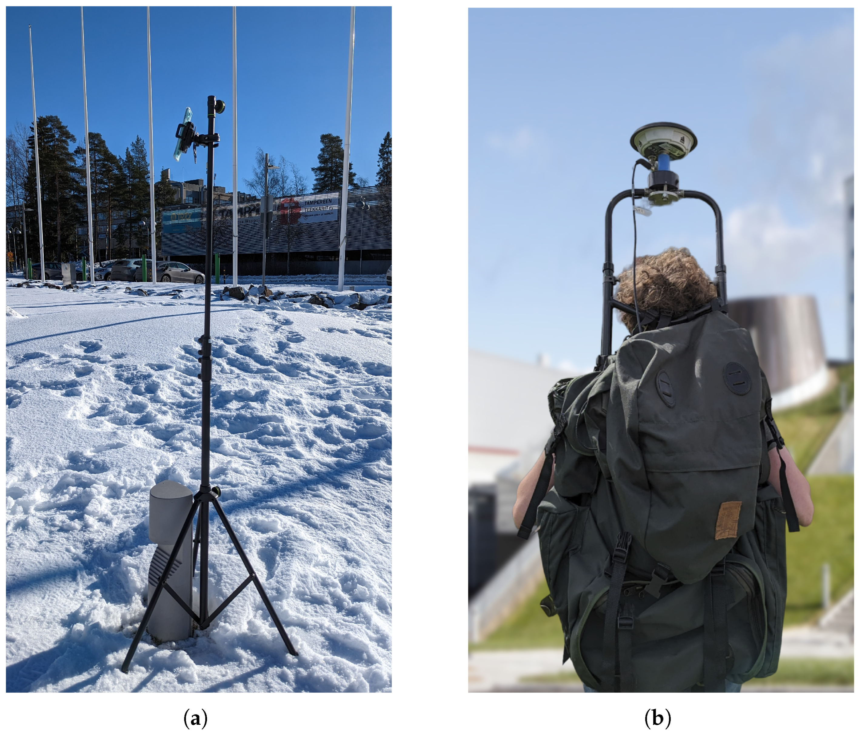
3.4. Survey Protocol

Based on the sections above, we can derive the survey protocol used for the acquisition and analysis of the devices, which is summarized in Figure 2.

Figure 2. Processing workflow for survey acquisition and processing.

For a proper comparison of the devices’ capacities, we define our reference/baseline to compare the measurements. During the process of evaluating the positioning capacities of the receivers, the most obvious benchmarking method is to find the reference coordinates of the surveyed locations. For static surveys, this can be easily defined after or before the survey by surveying the static location with a high-grade GNSS receiver. To minimize device disturbances, we used a tripod as represented in Figure 3a. For dynamic surveys, we used a backpack with an antenna mount on top as represented in Figure 3b. The used receiver was a Novatel PwrPak7 receiver connected to a Novatel GNSS-850 antenna. For the trajectory computations, we opted for Differential GNSS (DGNSS) computations, using the backpack a rover and our local GNSS station located on the university rooftop (Novatel GPS-703-GGG antenna, Septentrio PolaRx5 receiver) as a base. The total baseline between the devices ranges from a few hundred meters to a few kilometres, depending on the scenario. The DGNSS computations were performed using the open-source software RTKLib [38]; as these computations were needed only for the reference dynamic tracks, the DGNSS algorithms are not a part of our MimirAnalyzer software at present.

Figure 3. Description of the acquisition setups. (a) Static acquisition setup. (b) Backpack setup with reference receiver.

4. Dataset Description

In this section, we provide details on the dataset. We refer to it as a single “dataset” since it is provided at a single Zenodo link [7] but it is to be remembered that it contains several scenarios, both under static and dynamic conditions, and several Android devices. We start by detailing the logged sensors, then the survey scenarios will be presented and we provide a list of the performed surveys. Finally, we review the file structure of the dataset.

4.1. Scenarios and Environments

For our research purposes, we focused on pedestrian scenarios that are highly relevant in a variety of location-based applications such as studying mobility and migration patterns of workers or accessing various fundamental resources such as potable water (see LEDSOL project [6,19]), helping city planners to offer optimized services based on user location, or promoting more sustainable ways of transportation through optimized access to bikes, green lanes, or parks [39].

The university campus area and Hervanta center (a district in Tampere, Finland) offer an interesting and diverse environment for challenging positioning (i.e., open-sky, light forest, lake, suburban). While there are not many high buildings that could represent very harsh urban canyoning conditions, it is possible to recreate a partial blockage within the campus due to campus buildings (having between 3 and 10 floors). We have divided the surveys into three scenarios, all pedestrians with the conditions summarized in Table 2.

Table 2. Summary of the scenarios.

Defining the way the device is held or carried is also part of the scenario definition and crucial for future post-processing. Several studies [40,41] have shown how these carry modes determine the positioning models to use [40]. In [41], several carrying modes were assessed (e.g., texting, swinging, jacket pocket) and their effect on the inertial measurements, and consequently on the positioning solution, were reviewed.

In our study, two carry modes were reviewed in the dataset: (1) texting, where the device was held face up in front of the user; (2) backpack pocket, where the device was put in a stood-up orientation. These modes were chosen for their practical aspects, but also to understand how positioning might be affected by partial body blockage, as highlighted in [42]. Note that the smartwatch was placed on the left wrist (except S1). A representation of the scenario’s trajectories is displayed in Figure 4.

Figure 4. Maps of the scenarios’ trajectories. (a) S1; (b) S2; (c) S3; (d) S4.

4.1.1. Static Scenario (S1)

The first scenario is a long static acquisition (45 min), performed in a near-perfect open-sky environment. We took a small light post as a visible landmark to perform the acquisition with each device separately. The devices were placed on a stable tripod as represented in Figure 3a, allowing long acquisition with minimal disturbances. The tripod landmark was surveyed using our reference receiver to obtain its precise location. While the light post is relatively wide, this setup was assessed to be suitable for the purpose of the survey, given the positioning accuracy of the devices. Moreover, the positioning of the antenna phase centre is unknown for all Android devices, so a highly precise benchmark is not required.

The receiver taken as reference for the visibility analysis in this scenario is a base station located on top of the nearest building, about 100 m northeast. Figures and statistics of the survey are provided in Appendix B.

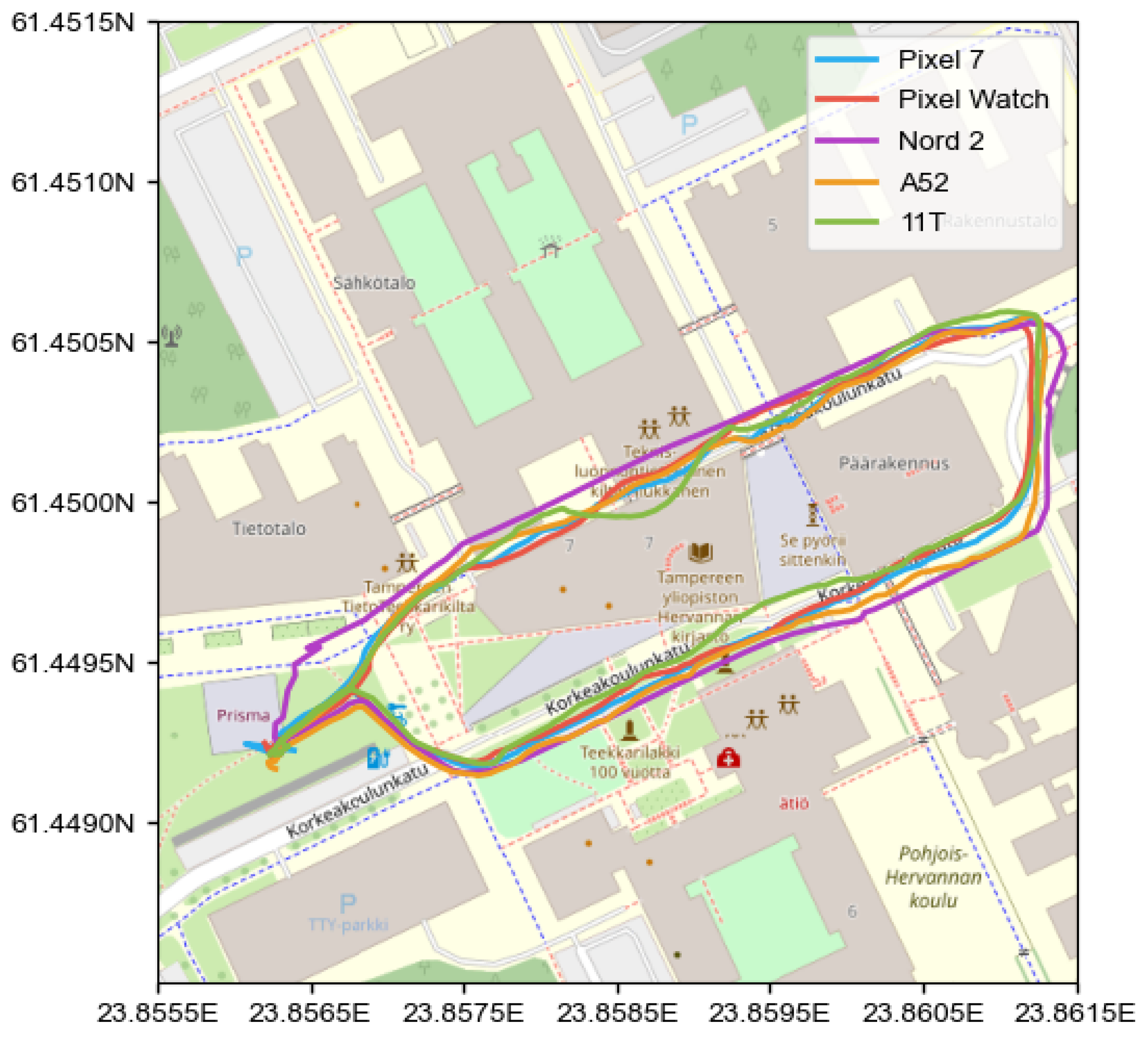
4.1.2. Short Dynamic Scenario with Urban-Canyoning (S2)

The second scenario is a short dynamic pedestrian acquisition (10 min), performed in heavy urban canyoning. The scenario starts and ends with a short (30 s) static acquisition over the landmark previously described in S1. This was performed to allow the convergence of the position and to ensure that every available signal was correctly tracked before the dynamic part started. The trajectory went from south to north. The southern part has relatively good visibility, with only some overpass bridges between the buildings. The northern part presents a very narrow alley between the buildings, with only a quazi-zenital sky view. The data were acquired separately, device by device, and the device was always placed in the right hand of the surveyor. The GPW was placed on the left wrist and acquired at the same time as the GP7, for comparison over the same GNSS chipset model. We used the backpack setup described in Section 3 as a reference receiver for each survey. Figures and statistics of the S2 survey are provided in Appendix C.

4.1.3. Dynamic Scenario in Urban Area (S3)

The third scenario is a dynamic pedestrian acquisition (45 min), performed in a light urban area. Similarly to S2, the S3 scenario starts and ends with a short static acquisition for the usual landmark. The southern part has good open-sky conditions, contrary to the northern part, which has tall buildings around it. Strong noise can be seen in the trajectory due to a tall building with an outside ceiling, which as expected leads to noisier measurements. Finally, the part located on the road shows a small underground tunnel with possible GNSS cutoffs. The data from all the devices were acquired at the same time; all devices were placed in separate side pockets of the backpack. This allows comparison of the devices over the exact same-scenario conditions. Figures and statistics of the S3 survey are provided in Appendix D.

4.1.4. Dynamic Scenario in Forest/Lake Area (S4)

The final scenario is a dynamic pedestrian acquisition (30 min), performed in a light forest area around a lake. Similarly to S2 and S3, the S4 scenario starts and ends with a short static acquisition. The scenario was chosen to evaluate the impact of vegetation and the lake on the measurement quality. Similarly to S3, the data from all the devices were acquired at the same time and all devices were carried along in the backpack. Figures and statistics of the S4 survey are provided in Appendix E.

4.2. List of the Surveys Performed

In total, twelve surveys were performed to acquire the dataset with the devices over all four scenarios. The surveys happened on different days throughout the year, and a summary is available in Table 3. Note that S1 surveys were acquired before the completion of the Mimir app. The measurements were acquired using the GNSSLogger app for smartphones, which explains the lack of barometer data. For S1 and S2, a separate survey was performed for each device, as the device was held in the right hand of the surveyor, thus allowing for only one device per survey. For S3 and S4, all devices were acquired at the same time in different pockets located on the side of the backpack.

Table 3. Summary of the surveys performed and sensors logged.

4.3. File Structure

Multiple types of files are present inside the dataset. For the reference data, we provide the observation data in Novatel proprietary log file format, and the RINEX files extracted using Novatel Application Suite software. The observations from the base station are provided in RINEX files.

For Android devices, the raw logs are produced in a simple CSV format. This format was chosen to allow compatibility with the GNSSLogger app (presented in Section 3.3). Each line of the CSV file represents the data from a sensor at a specific timestamp. While multiple clocks might be defined inside the device (e.g., GNSS clock, system clock), all entries provide two timestamps: a UTC time in Unix format based on the global system clock, and a time counter since the last time the smart device was booted. The former is used for temporal indication but it might not be very accurate, as explained in Android documentation [43], and it is recommended to use the latter for more accurate time intervals.

We note that, while it is possible to request a specific sampling frequency through the Android API, our empirical experiments have shown that the accuracy of the sampling clock can be poor. Requesting for a too high or too slow sampling interval might lead to truncated sampling, based on the physical limitation of the sensor. It is recommended to interpolate the values of a log to the wanted sampling frequency before any processing is performed. The time information discussed above should be sufficient for accurate clock alignment between the sensors and with the GNSS clock.

4.4. Sensors Summary

Multiple sensor types were logged during the surveys and are listed below:

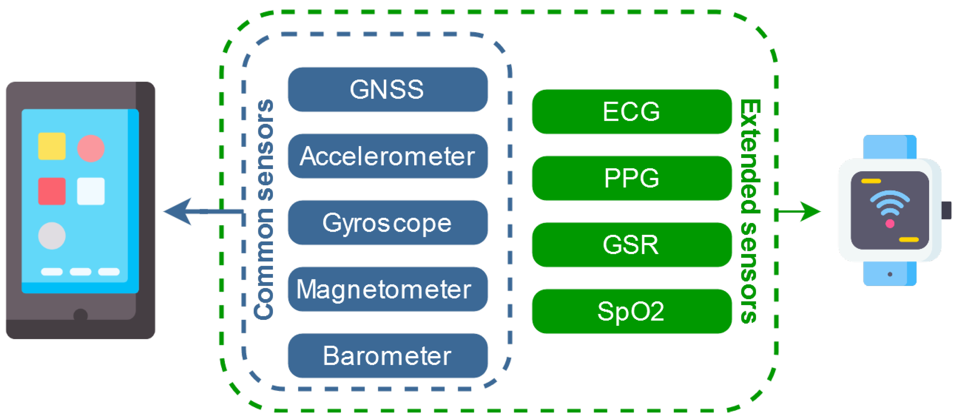
GNSS measurements that can be associated with multiple line entries in the log file: (1) location measurements (latitude, longitude, altitude) provided by the phone, from different providers; (2) raw GNSS measurements, as described in [11,44]; (3) navigation messages, as provided by the Android API and decoded by the GNSS receiver (i.e., not from another network channel).
INS measurements, composed of two type of sensors: accelerometers, providing linear acceleration measurements, and gyroscopes, providing rotational acceleration measurements. In total, we have on each mobile device three accelerometers and three gyroscopes, placed on the three orthogonal axes (X, Y, Z), allowing re-composition of a relative motion in three dimensions.
Additionally, an INS often include magnetometers, which measures the magnetic field (similar to a magnetic compass). The magnetometer enables the absolute orientation and estimation of the INS drifts [45]. Similarly to the INS measurements, three magnetometers allow the measurement of the magnetic field in three dimensions. All this information can be put together to form a low-grade INS system to be combined with GNSS measurements [1,2,45]. In the Android documentation, these sensors are regrouped under the term “motion sensors”.
Barometer measurements, related to the atmospheric pressure can be converted into altitude. As GNSS is known to have low precision in the up/vertical direction due to the geometry of a GNSS system, a fusion of GNSS/Barometer measurements is often seen in positioning applications [46].

All sensor entries are located in the same file, the first column containing the tag identifying the measurement type. The entry order follows the timeline of the sensor event reception. As different sensors provide different data, a header at the beginning of the files recalls the CSV columns for each sensor type. Motion sensors can also be retrieved “uncalibrated”, with their biases provided but not applied. In total, there are 10 different possible tags in the file. Table A1 in Appendix A provides a summary of each logged sensor measurement; additional details can be found directly in the Android developer documentation [43].

5. Performance Metrics

For the analysis of the collected raw data, we have divided our study into three sections for each scenario: (1) positioning, assessing the native capacity of the device; (2) visibility, assessing the constellations/frequencies visible by each device; (3) measurements, assessing the raw GNSS observables’ precision, which is relevant to advanced positioning applications. In this section, we explain the performance metrics chosen to evaluate these aspects in each scenario.

5.1. Positioning

The Android API give access to different location providers, with different degrees of precision: NLP, Network Location Provider, related to the mobile network position (coarse precision); GPS, as provided by the GNSS chipset (standard precision); FSL, Fused Location Provider (best precision); in this paper, we focused on the GPS provider locations only, as provided by the phone. We did not perform any post-processing of the positions, nor computed the positions using advanced positioning techniques (e.g., sensor fusion, DGNSS, PPP). Instead, for positioning quality review, we computed the position errors in the east/north/up (ENU) direction, based on the reference receiver used in each scenario (see Section 3). These errors can be reviewed in two graphs, an overall map and ENU error against time, as well as statistic tables.

5.2. Visibility

Throughout our analysis, we realized that the Android API provides an event at a regular sampling rate (i.e., 1 Hz), while the measurements per satellite are not regular. Gaps of several seconds (1–5 s) can be seen for certain satellites, leading to the idea that the device performs some kind of sequential tracking. The signal stops being tracked by the receiver for a certain amount of time to concentrate on the tracking of another signal. The receiver then comes back to the first signal to converge again, and avoids the signal falling out of the tracking loop. The most probable reason is to limit the energy consumption, and possibly to enable more signal tracking than supported by the number of channels available in hardware. This phenomenon has been seen on every device, even with a different number of total visible signals per epoch.

Today, the GNSS tracking is often limited to the four major constellations (GPS, GLONASS, Galileo, BeiDou), with dual-frequency (L1/L5) for the most advanced ones. Some Android devices do support some other satellite-based systems such as IRNSS and QZSS. However, none of the devices reviewed showed the reception of SBAS satellites. Consequently, while the geodesic-grade receivers used as a reference allowed the coverage of almost all constellations and frequency bands, we limited our comparative analysis only to the signal available in the Android devices, for a fairer comparison.

Constellations in the results are named based on their RINEX code, as defined in [47]: G (GPS), R (GLONASS), E (Galileo), C (BeiDou), I (IRNSS) and J (QZSS). Similarly, frequencies and signals are simplified to L1 (∼1575.42 MHz) and L5 (∼1176.45 MHz). For comparison with the reference receiver, we extracted the following signals based on RINEX definition: L1 ⇒ (L1C, L1L), L5 ⇒ (L5Q, L2I, L5P, L5A).

To best assess the satellite’s visibility of the devices, we provide two types of graphs: the number of signals seen at each epoch w.r.t time, and bar graphs with the total amount of unique signals seen during the whole scenario. For the latter, we also add the total amount of signals seen by the reference receiver (the left bar) to compare against each device (the right bar). The bar graphs come in two variants: one per constellation and one per frequency. We also provide a summary table comparing the percentage of visible signals compared to the reference receiver.

5.3. Measurements

Four observations are used in GNSS positioning: pseudorange, carrier phase, Doppler shift, and SNR. The last two are provided straightforwardly in the GNSS event of the Android API; however, the pseudoranges and the carrier-phase data require some post-processing to be usable in a typical GNSS algorithm.

As described in [44], the pseudorange needs to be constructed based on the received and transmitted times given in the event. Several checks of the tracking state should be performed for each constellation to ensure correct measurements. In our analysis, we used the instructions provided by [44], but we only checked for adequate code lock and Time of Week (TOW) decoded. The carrier phases in Android devices are provided as “Accumulated Delta Ranges”, which correspond to the regular carrier-phase measurements multiplied by the wavelength of the GNSS signal, thus in meter units and not in cycle units.

For both the pseudoranges and the carrier phases, we performed a double time difference on the measurements, similarly to [10]. The double time difference allows for discarding the residual drift induced by the velocity changes, leaving only the acceleration changes which are assumed too small for both satellites and users in our study cases. It also reduces or cancels out some errors present in the GNSS measurements, such as atmospheric error or satellite orbit/clock error, as two consecutive measurements at a regular small rate (here 1 Hz) should be tainted by similar errors. Consequently, the error left can be assumed to be related mostly to the receiver tracking noise. While other papers have used different error estimations for measurements, such as the Code–Minus–Carrier combination [11,12], the double time difference method showed adequate results for a preliminary analysis. For Doppler measurements, only one time difference is needed as the measurement is already a velocity/rate estimation. For C/N0, it is more interesting to study its value range; thus, there is no difference in performance.

The results are provided as logged, with minimum filtering of the data for a more realistic analysis. However, to minimize the number of outliers and end up with biased statistics, we filtered some of the measurements based on a threshold, as a basic navigation filter would do. The threshold values were chosen empirically, based on the standard deviation and expected precision of each type of data. Consequently, the thresholds were set as follows: pseudorange ⇒ 300 m, Doppler ⇒ 30 m and phase ⇒ 30 m.

For each scenario, a statistic table for each GNSS measurement is provided, along with the percentage of measurements included/removed from the filter. For pseudoranges, Doppler and phase errors, we used box plot graphs to represent the different statistics. For Carrier-to-Noise ratio (C/N0), we choose to represent the data in “violin plots”, which are mostly similar to box plots but provide additional information on the data distribution. It is specifically interesting to study the L1/L5 differences and the range of CN0 values.

6. Results

In this section, we review each scenario and provide a first analysis of the data. We do not review in detail the content of each figure/table provided in the appendices, as they can be redundant for many scenarios. Instead, we summarize the observations from all scenarios in three sections related to positioning, visibility and measurement analysis, and only show the relevant figures within this section. A comprehensive summary of the performance metrics is available for each scenario in Appendix B (S1), Appendix C (S2), Appendix D (S3) and Appendix E (S4). For more details on the data, the results presented in this study are accessible in the Jupyter Notebook file available on MimirAnalyzer’s Github.

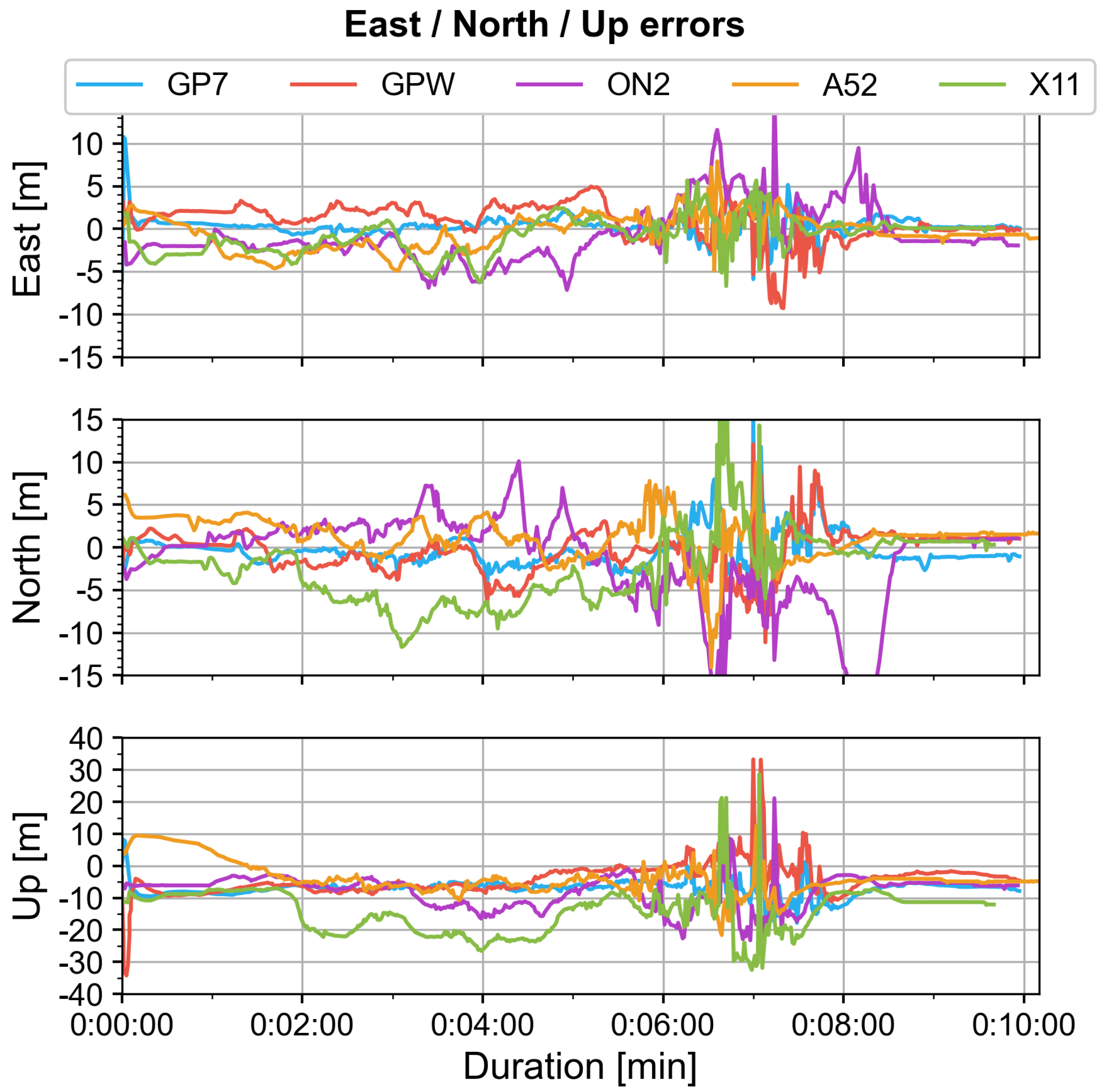
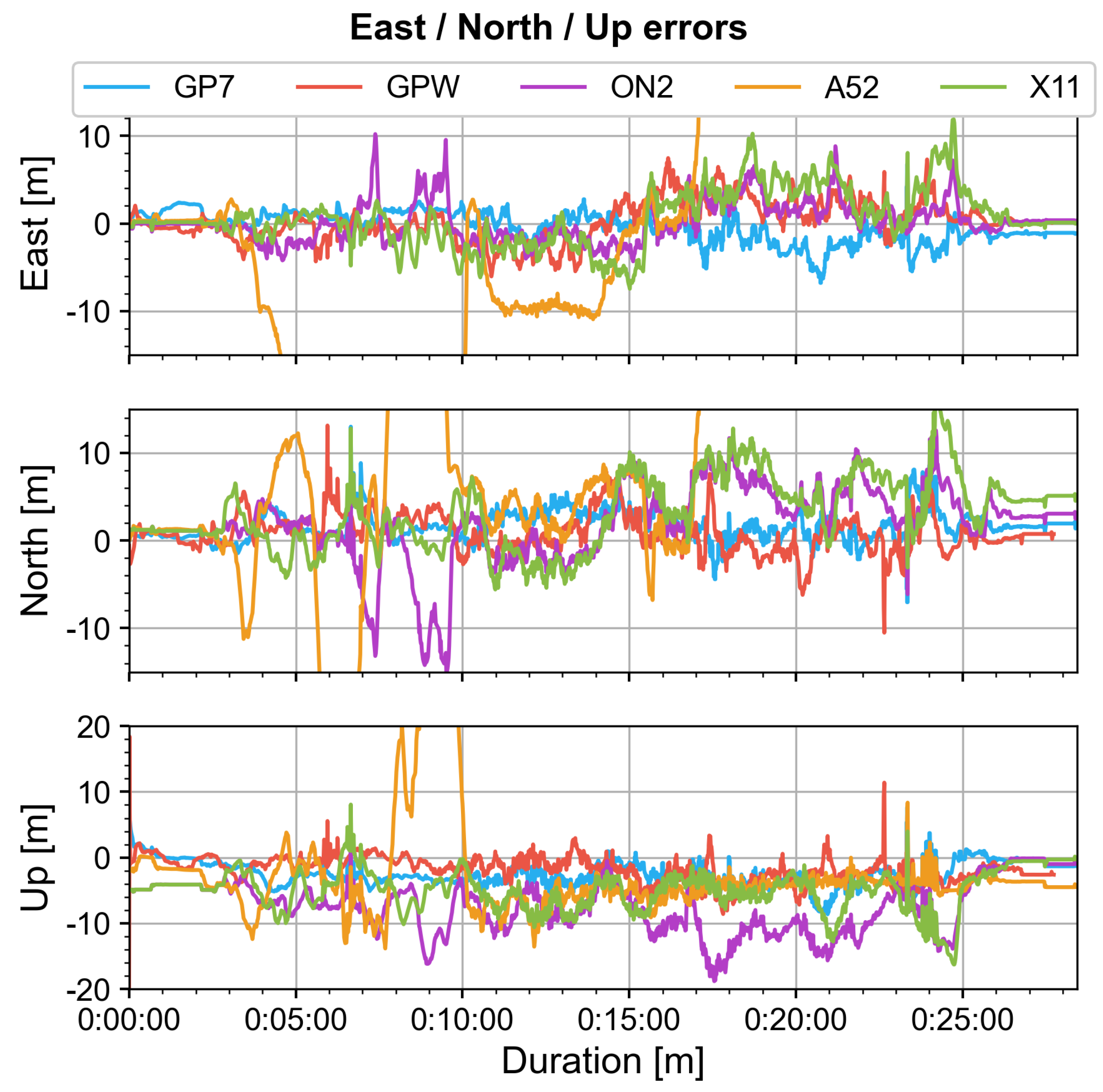
6.1. Positioning Analysis

All the devices showed signs of heavy filtering (e.g., Kalman Filter) inside their proprietary navigation algorithms. The locations provided by the GNSS chipset inside each Android device followed a stringent user dynamic, which allowed a very smooth trajectory. This heavy filtering is even more apparent during the static survey (S1). In Figure 5 and Figure 6, the GP7 and GPW seem to be converging around the static position, with a looser prediction model. However, other devices such as the ON2 and X11 report a constant position throughout the whole survey, which explains the very small standard deviation. This can probably be explained by a more highly constrained motion model based on user dynamic assessment performed by the receiver internally.

Figure 5. Two−dimensional error in East and North (S1).

Figure 6. East−North−Up error (S1).

During the dynamic surveys, all the devices provided consistently good positioning with relatively small divergence from the ground truth and within each other. Certain discrepancies can, however, be found with the A52 device during S3 (Figure 7) and S4 (Figure 8), leading to wrong positioning before quickly re-converging to the actual user position. Yet, this was not seen during S2, with a much more challenging signal environment, making it hard to assess the actual cause for such drift in positioning.

Figure 7. Two−dimensional error in east/north (S3).

Figure 8. Two−dimensional error in east/north (S4).

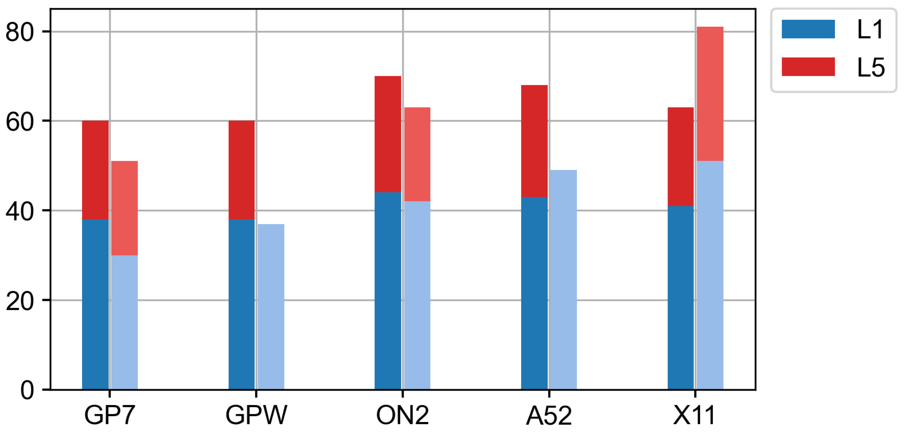
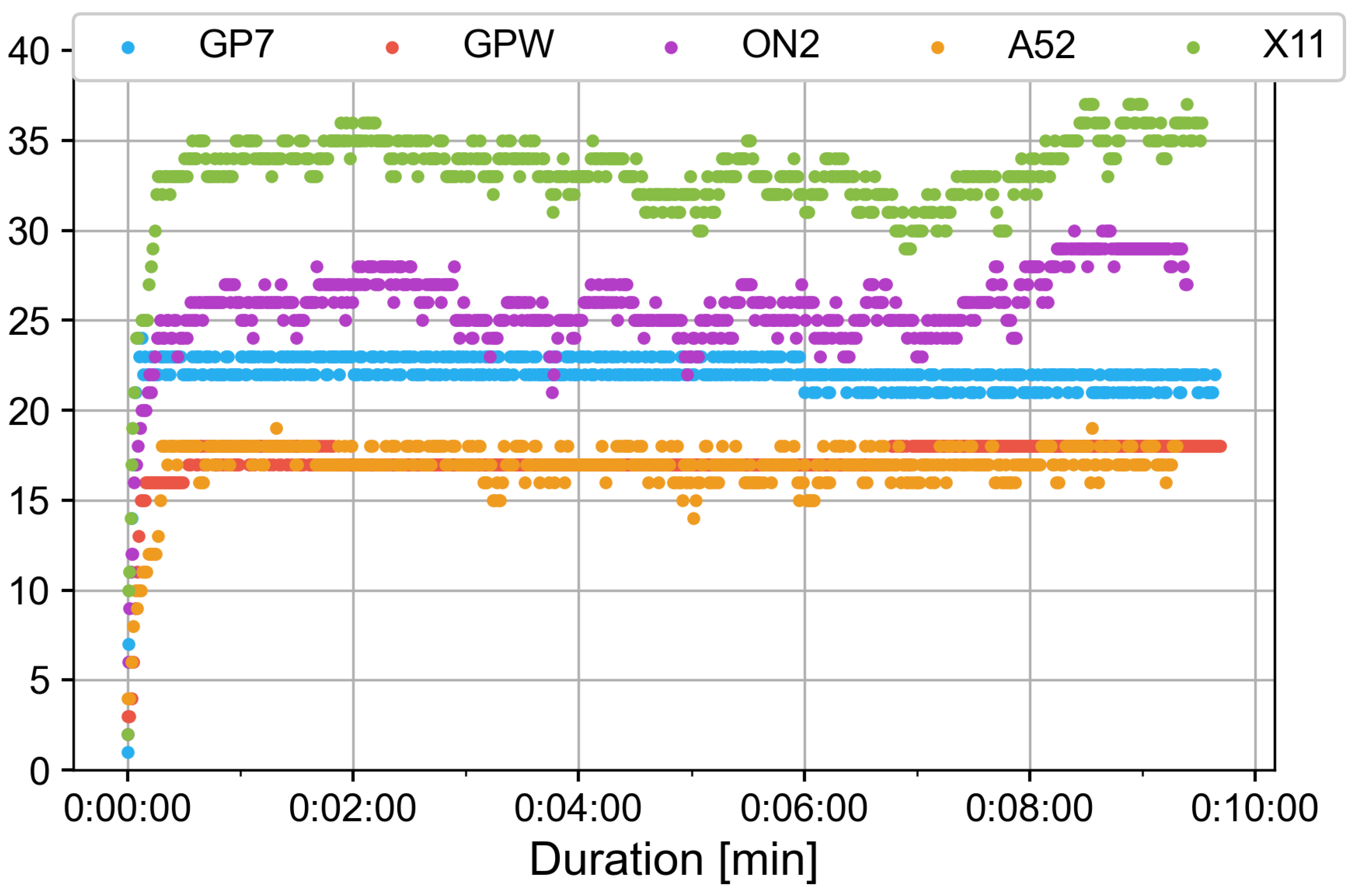
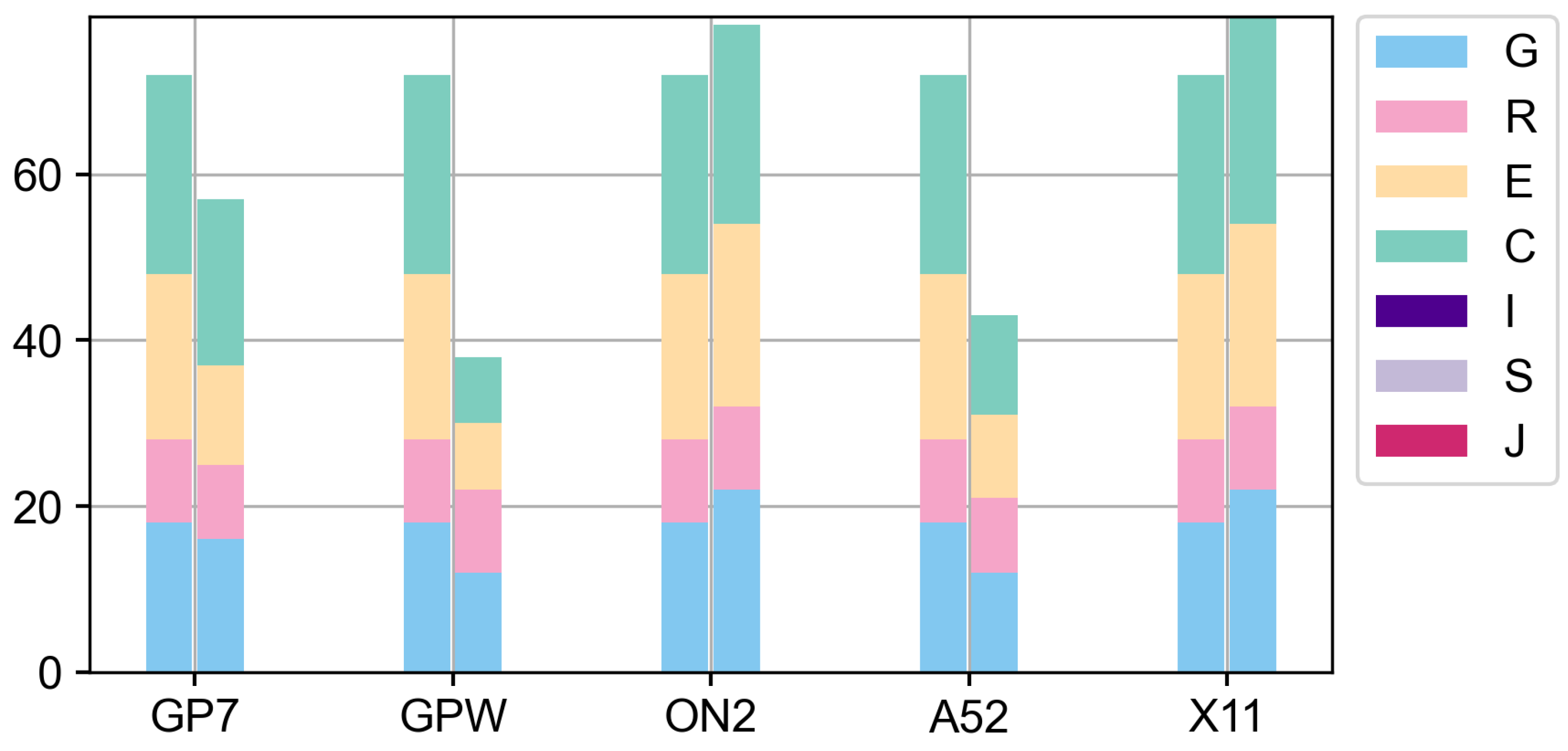
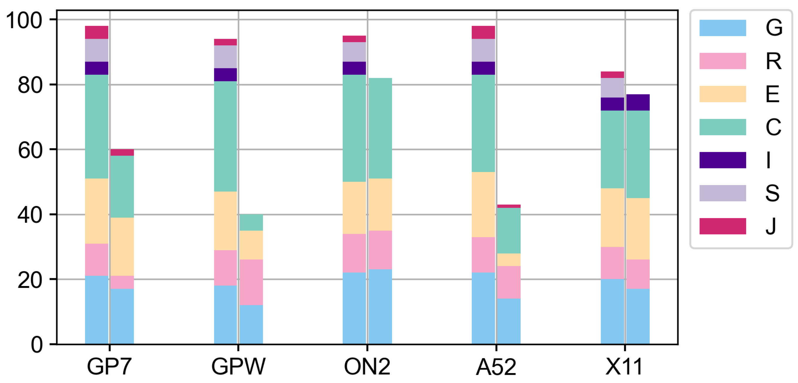
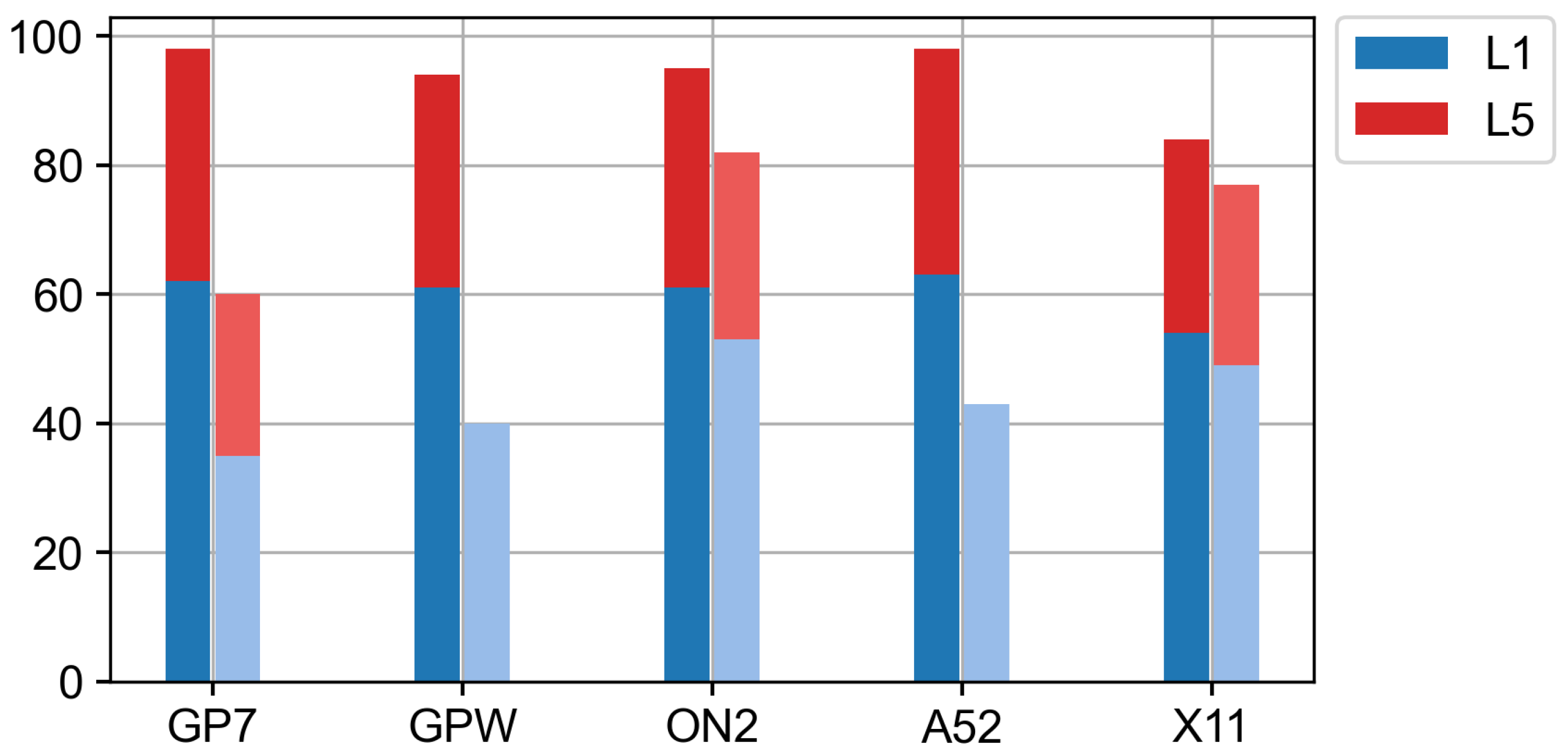
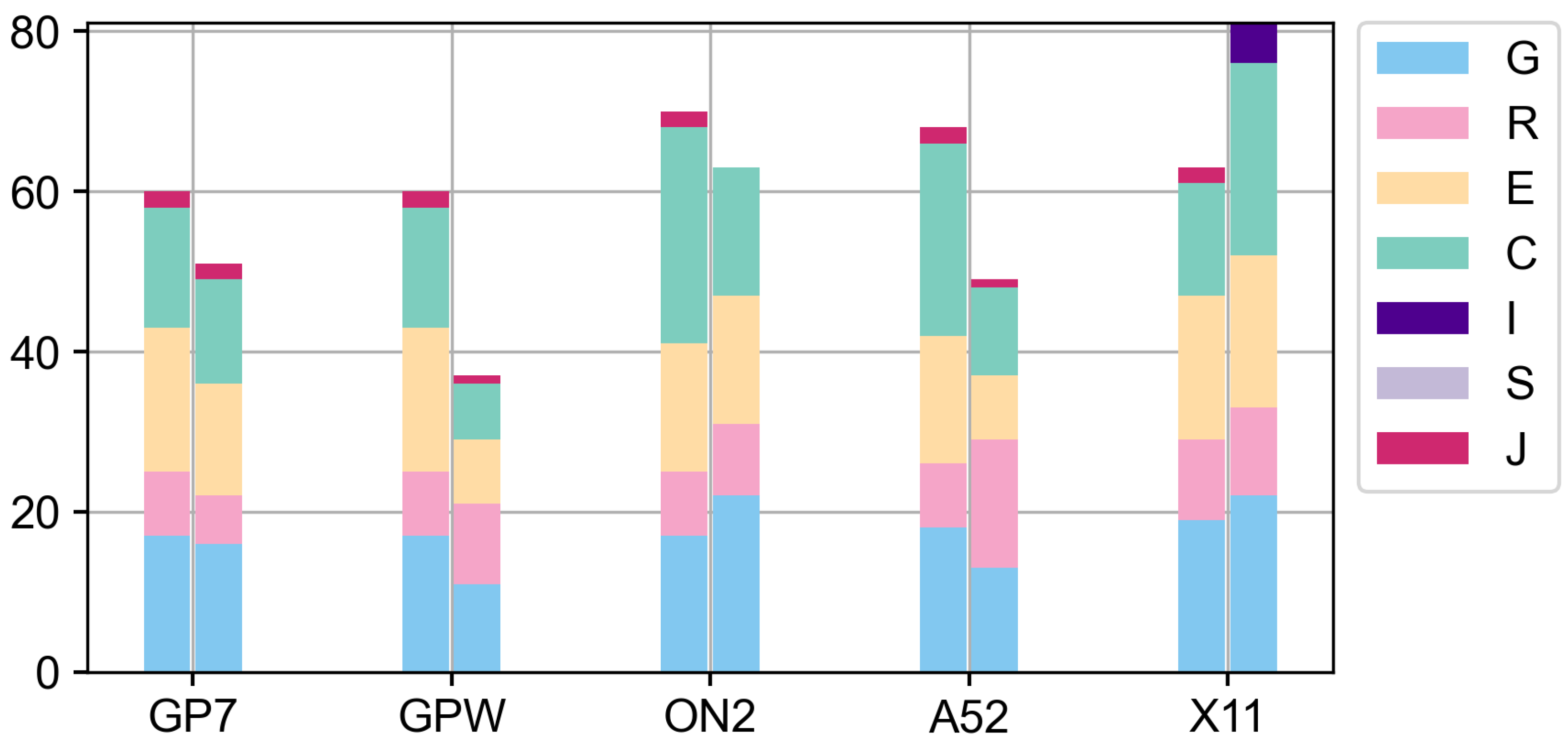
6.2. Visibility Analysis

Overall, dual-frequency devices showed great visibility performances, capturing most of the signals compared to the receiver. In certain cases, some devices have even reported more satellites than the reference receiver. In these cases, the satellites were actually flagged as unhealthy and were not included by the reference receiver, contrary to the devices that included any measurement received in the log file. As the positioning solution presented here is computed by the device itself, not all the visible satellites in the raw data are likely to be used by the devices and this is a topic of future investigation; in any case, the effect on navigation should be minimal if not in a highly constrained environment.

The visibility analysis would benefit from additional comparisons that should be performed to compare the C/N0 levels against satellites’ elevation w.r.t. the reference receiver. Mono-frequency devices showed very good results in capturing the L1 frequency. Yet, given that all the major constellations today transmit L5 signals, it significantly reduces the amount the total amount of signals seen by the device. An interesting case is the GPW smartwatch, as it should integrate the same GNSS chipset as the GP7 smartphone, but did not show any dual-frequency measurements contrary to GP7. Nevertheless, comparing positioning results between GPW and GP7 showed similar results in all scenario cases.

The most remarkable result seen in smart devices is the capacity to alternate ON/OFF tracking of signals. It allows more signals to be tracked concurrently and optimizes power consumption. Concurrent tracking is not a new concept, as it was used in the very first GNSS receiver with limited hardware channel, and probably is still used today in other receivers. Yet, the effects are directly visible here in the measurements.

The downside of concurrent tracking is it results in many gaps in the measurements. To overcome this issue, one could perform interpolation of the measurements to have a regular rate, as the gaps are relatively short. In our processing, we did not perform any interpolation as it was not needed for our presented analysis. Advanced processing techniques, such as PPP, might indeed require adaptation to their algorithms to account for such measurement discrepancies and should be reviewed for future research.

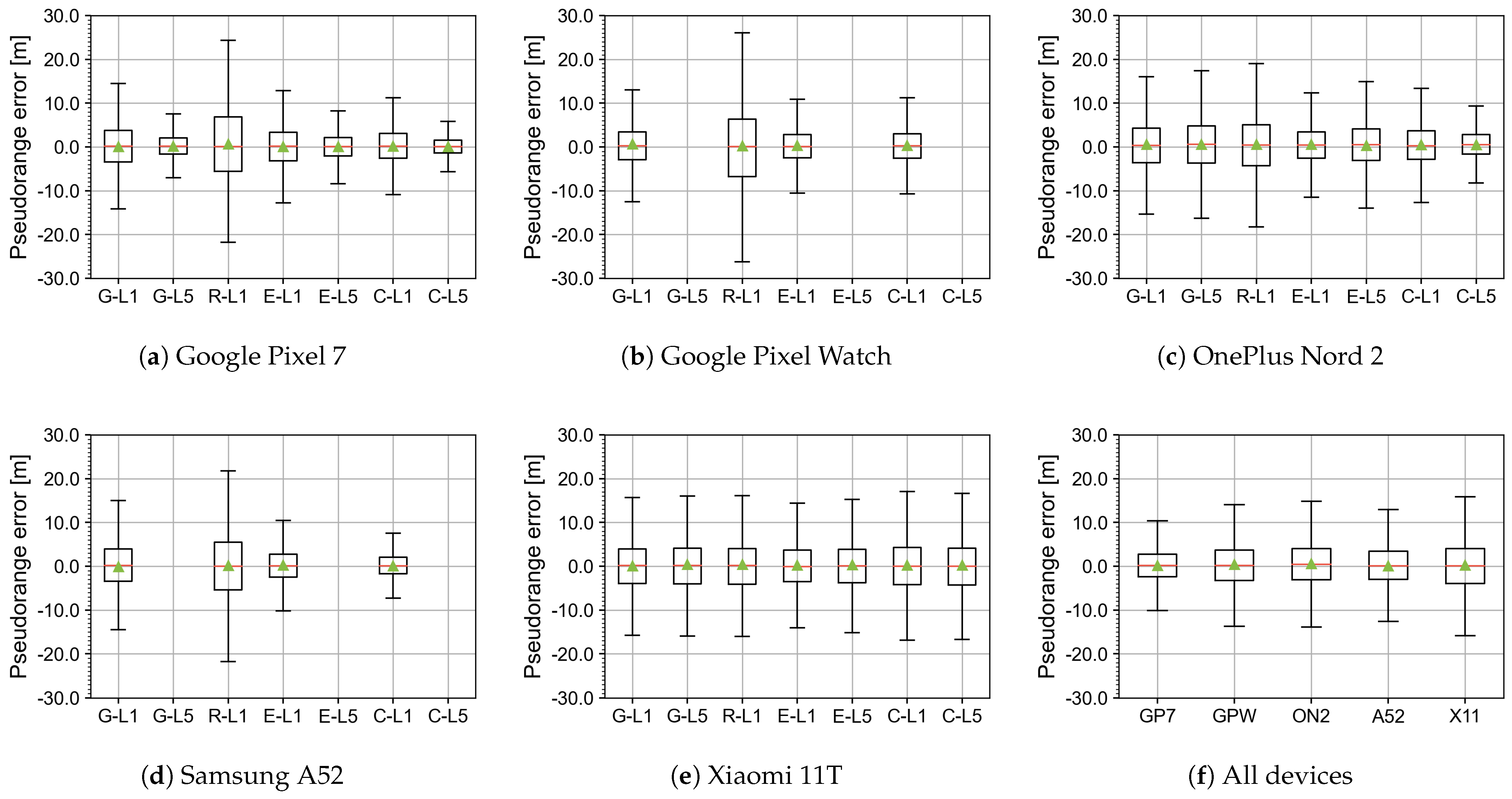
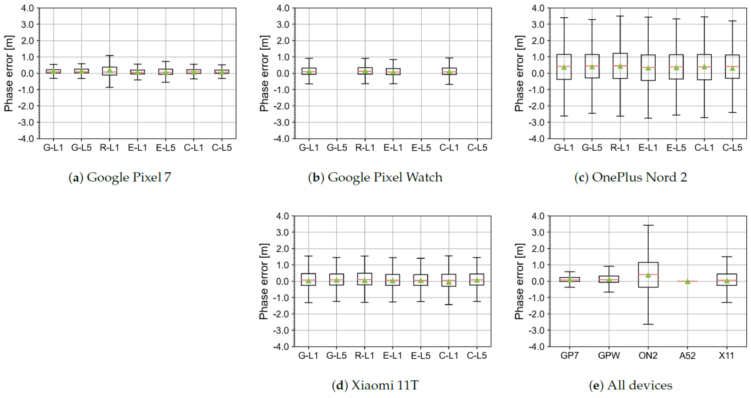
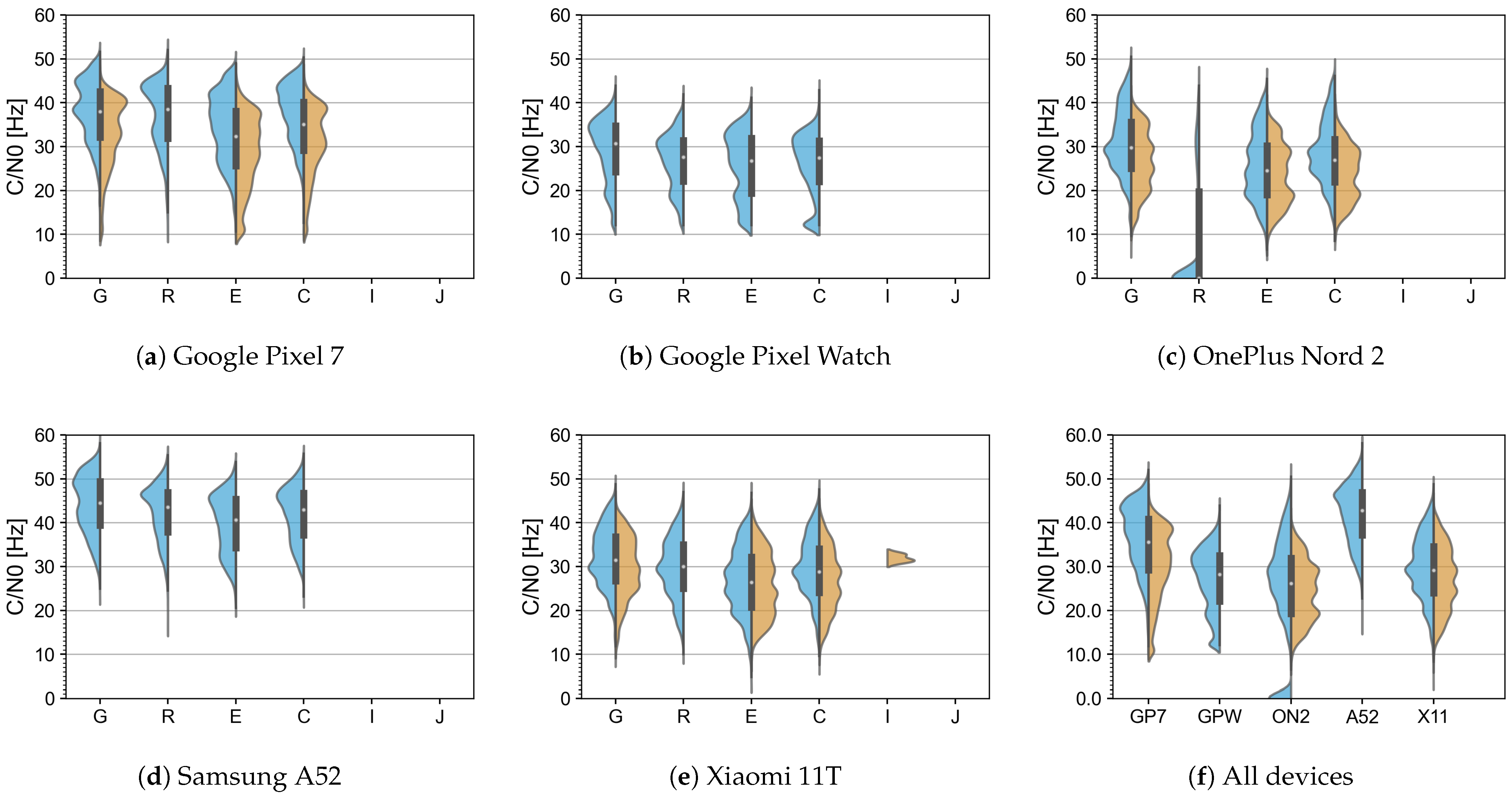
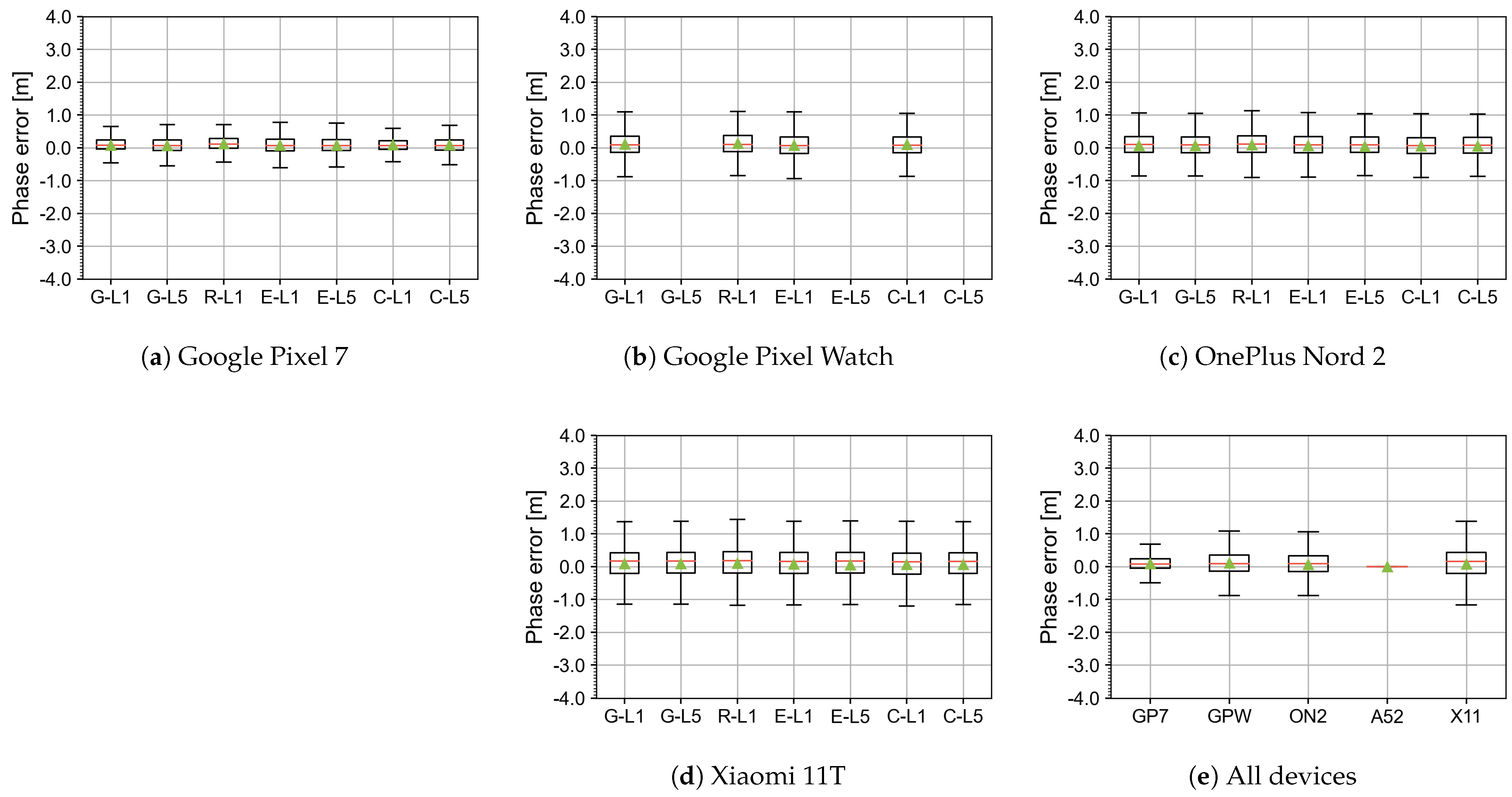
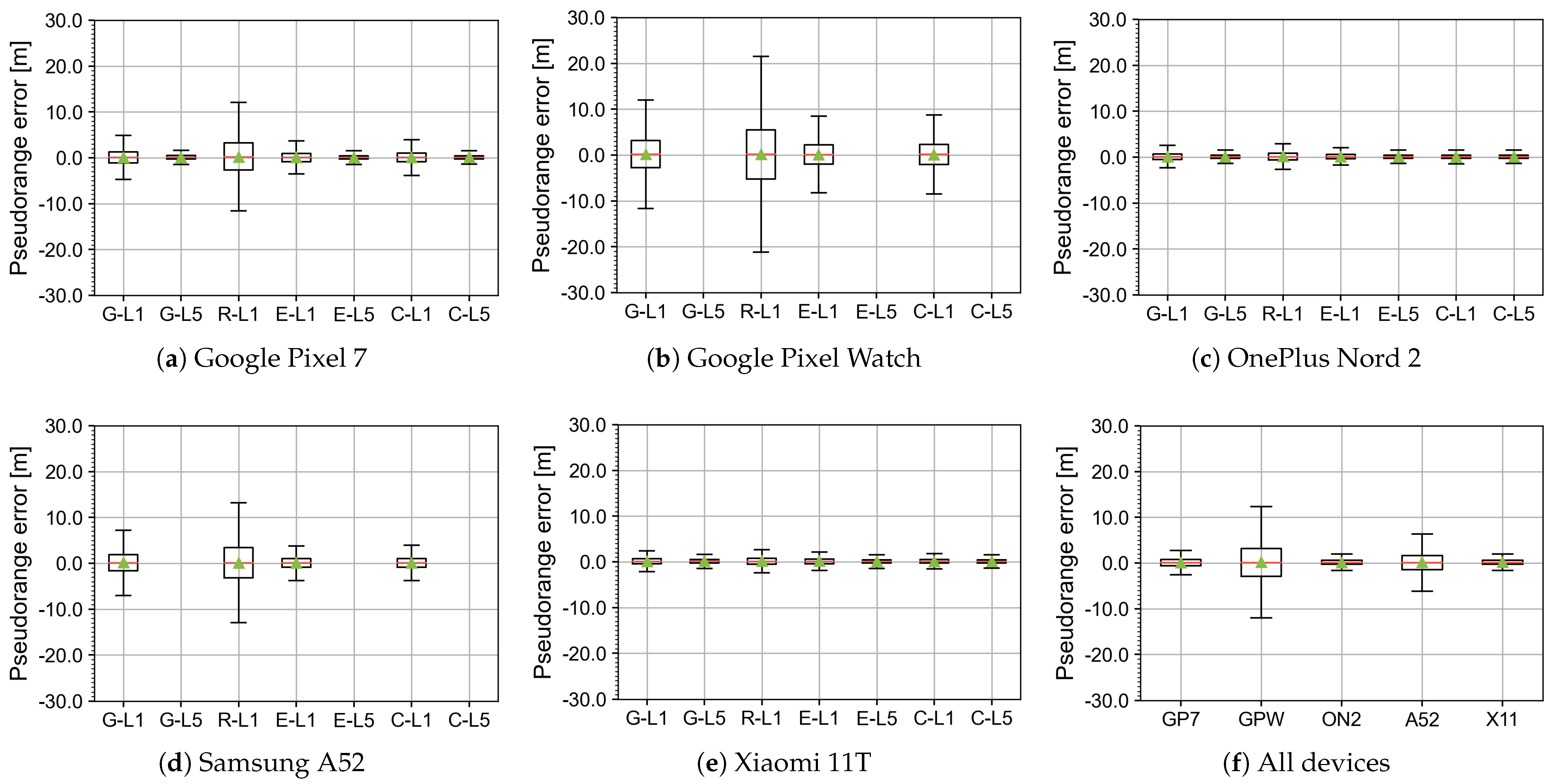
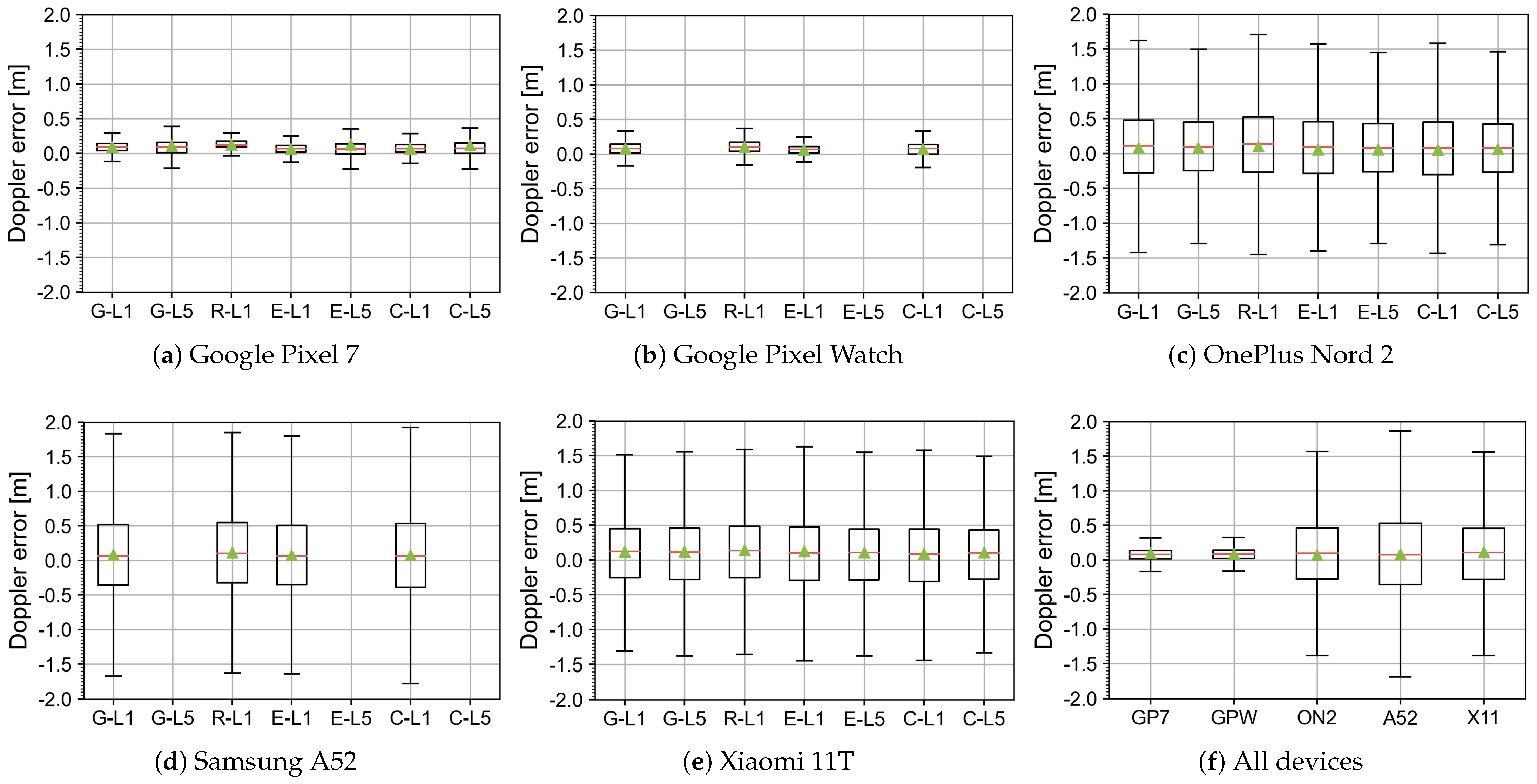
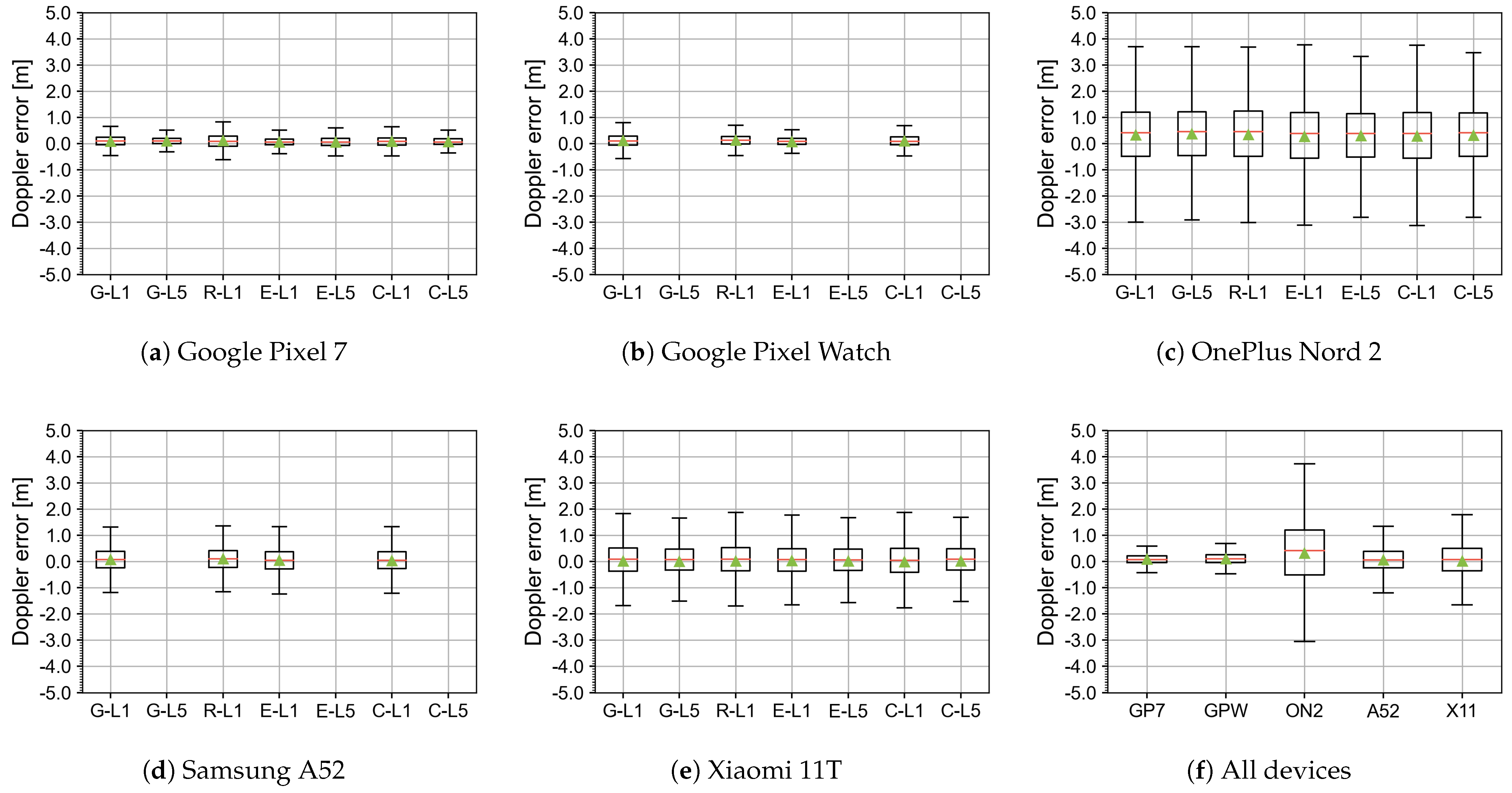
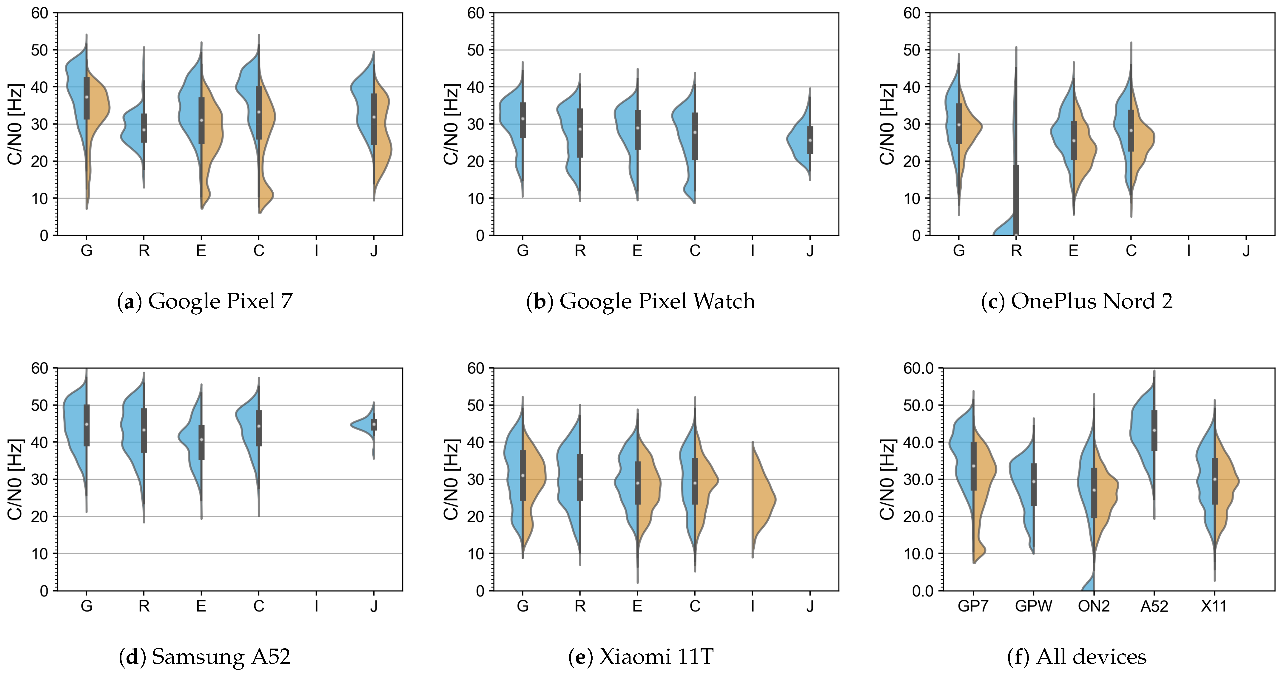
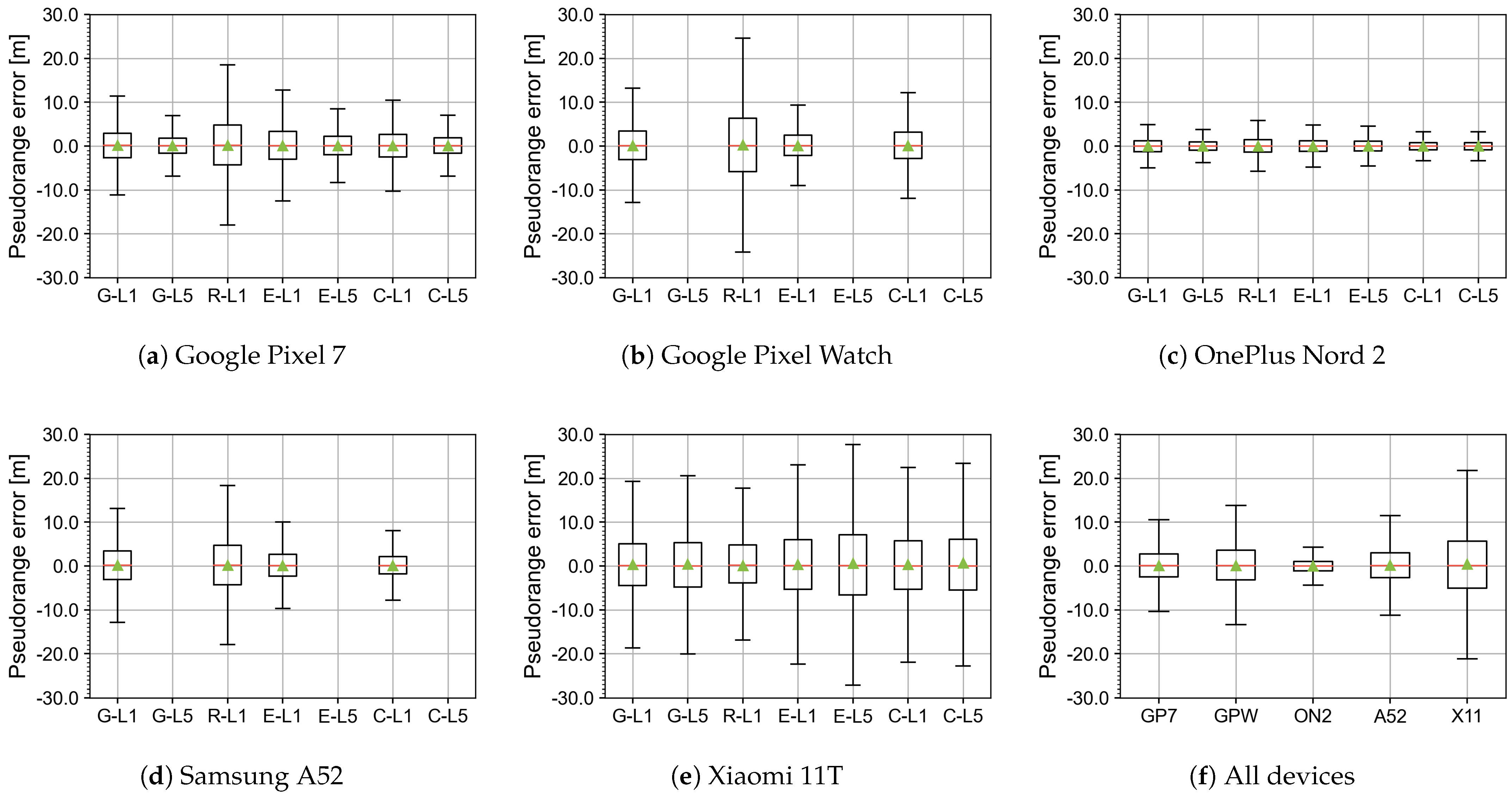
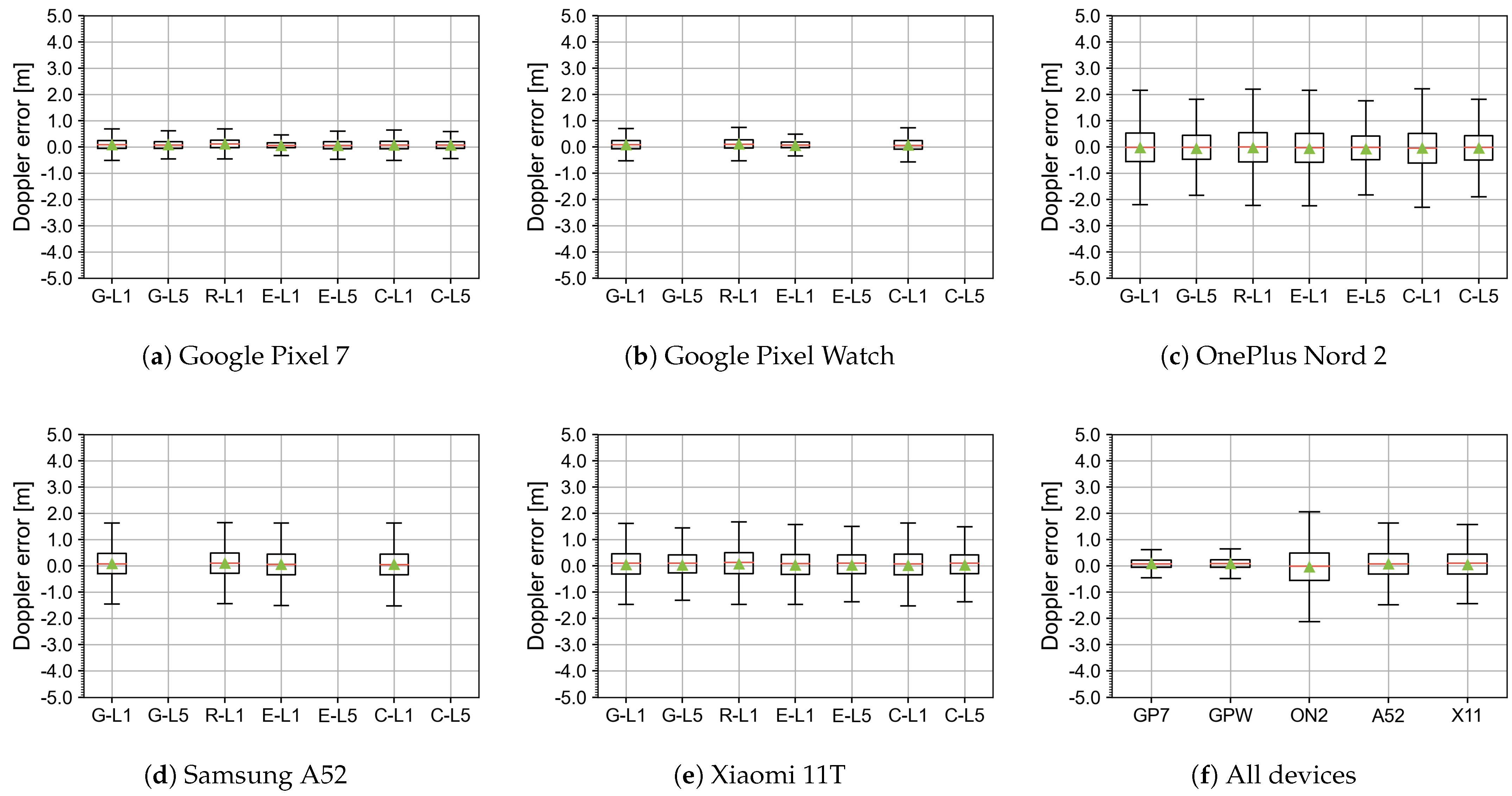
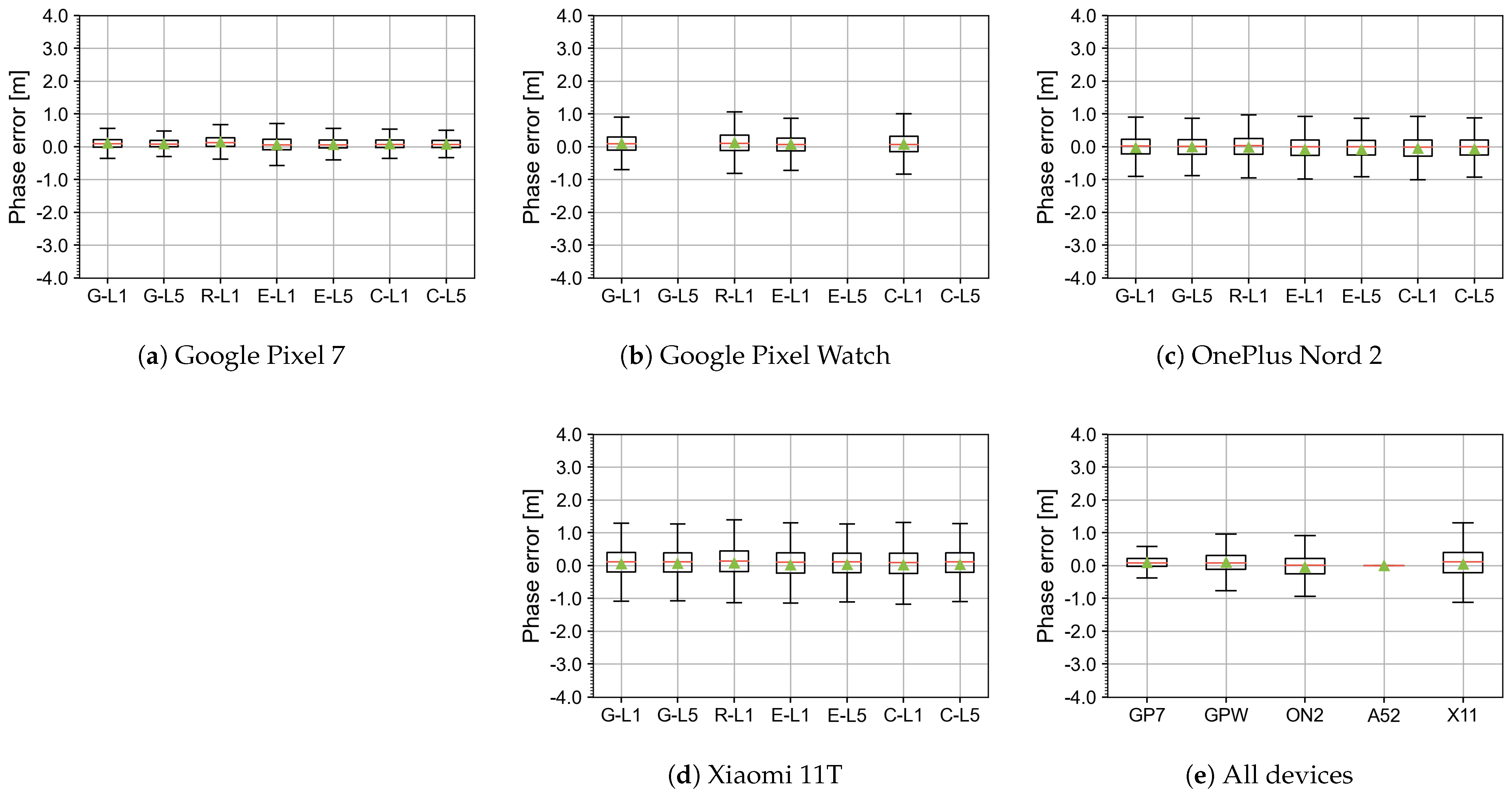
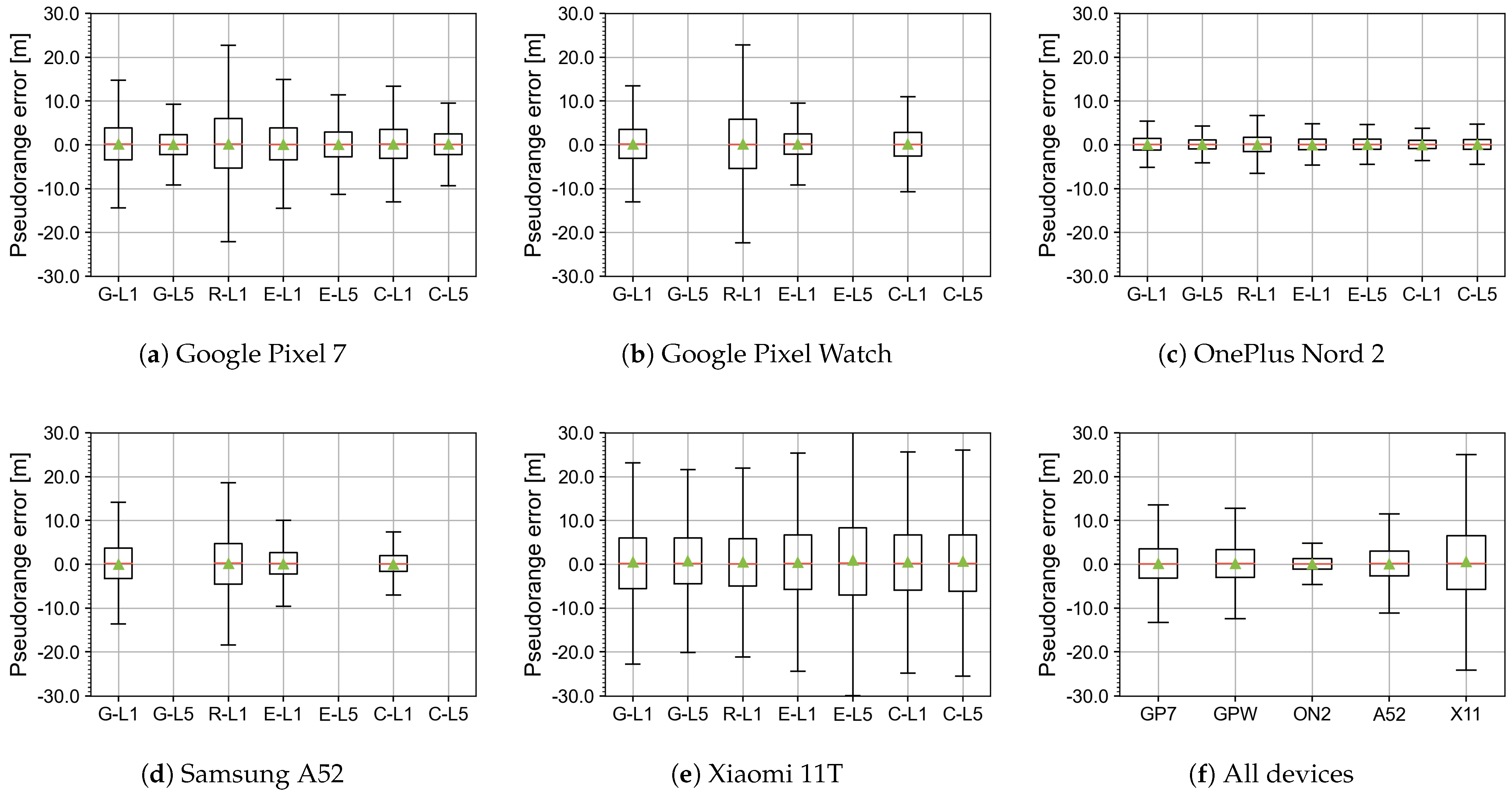
6.3. Measurements Analysis

All measurement errors were found to be very consistent throughout all the scenarios, with higher noise during dynamic scenarios compared to the static ones. As mentioned before, measurements were filtered to avoid biases in statistics due to outliers. Yet, a more thorough analysis of these outliers would be interesting to better understand the resilience of devices in different environments. Moreover, Android provides a certain amount of flags on code and phase tracking quality, as well as multipath flags, directly within the API. These flags have not been used in this analysis but should be checked for more advanced positioning computations, as assessed in previous studies [48,49].

Pseudoranges errors from certain devices (i.e., ON2 and X11) appeared to have a much smaller dispersion. A possible explanation could be pseudorange smoothing using Doppler or phase measurements, as this technique is often used to reduce pseudorange noise [9].

Regarding Doppler measurements, a relatively small standard deviation was observed for GP7 and GPW, compared to the other devices. Both Doppler and phase measurements showed a tendency for a small positive, regardless of the devices. While the exact reason is not clear, it is believed to be due to the time-differencing operations performed to obtain the error measurements, as described in Section 5.3. Future research should review the effects on measurements, possibly using other techniques such as the Code–Minus–Carrier combination (see Section 5.3).

C/N0 comparison showed a distinct drop in their values between L1 and L5 tracking in all devices. Yet, L5 signals are designed with a higher minimum received power [50], which shows that smart device hardware is not optimized yet for the reception of this additional frequency. Further comparison between frequencies should be performed to further assess the impact on the measurement quality.

7. Discussion and Future Work

7.1. A Suitable Reference Definition

During the processing of dynamic surveys, we realized that the reference trajectory actually looked noisier than the one from the devices. The reference trajectory was computed in DGNSS baser/rover setup, as described in Section 3 and DGNSS computations were performed using the open-source software RTKlib. Even with DGNSS, the errors of the reference rise significantly in challenging environments, due to the limited number of satellites visible and multipath errors. Consequently, the statistics tables of position errors presented in the appendices need to be reviewed with this consideration in mind.

Nevertheless, we do not attribute such error to the receiver, but to the processing itself. As navigation algorithms inside Android devices are proprietary, it is difficult to assess the filtering algorithms and parameters. Consequently, simple DGNSS processing as performed in RTKlib is not sufficient and more advanced processing should probably be performed on the reference data to better assess the positioning capacities of each device. In our next research developments, we are planning to integrate the positioning processing (i.e., Kalman Filter) within the MimirAnalyser software to improve the reference trajectory processing.

Moreover, the dataset would benefit from an INS coupled with the reference receiver setup. It would enable better processing for the reference trajectory, and the INS measurements could be compared against the INS recordings from the smart devices. However, INS methods require alignments of the different devices’ frames, which could prove challenging. It is the main reason why using a combined GNSS/INS solution for the reference trajectories was left out of this analysis. Future work should look into the feasibility of enhancing the reference trajectories with INS measurements.

7.2. The Android Platform for Research

Sensor logging and measurement quality assessment on Android come with a set of challenges. During our research, we discovered that while there are numerous apps existing today for sensor logging, there were none suitable to log every sensor available on smartphones/smartwatches. Apps related to GNSS logging (e.g., GNSSlogger) only concentrate on motion-related sensors and do not allow customization on the sensor parameters. Therefore, we had to develop a new application to fit our research needs, which required a certain knowledge of Android development. As this app is open-source, it can be re-used and enhanced by the research community to be used in new applications. Alternatively, the dataset produced through this research can be used as also provided under open-source license.

While the Android platform is not easy to access, it does allow common and easy access to raw measurements from sensors, which would require heavier hardware developments otherwise. Power management inside the device can prove challenging, as the system itself might perform automatic duty-cycling strategies which can impact sensor logging, which can be even trickier on smartwatches. An easy workaround for Mimir was to prevent screen lock and keep the app awake to avoid duty-cycling by the system. Yet, the assessment of power consumption is part of the future work for this research to review the impact of advanced positioning techniques on the battery life of a device.

Regarding the smartwatch, developments have proven to be quite similar to the smartphone case. The common API made the development of a common Android library possible, avoiding the need for redundant code developments specific to each platform. Data extraction was, however, a bit more challenging, as the smartwatch did not have any USB port. Consequently, the data had to be extracted through WiFi and with the help of the Android development software. Future developments on the Mimir app will try to improve the interactivity between smartphone and smartwatch so that the data can be uploaded through a companion phone first before being extracted by USB.

While the smartwatch offers a new playground for health-related sensors, they have not been reviewed here as outside the scope of this study. It has to be noted, however, that extraction of these sensor data is implemented in the Mimir app, and future research will also focus on reviewing their quality. As smartwatches can be very interesting for long-term study of patients, focus will be given on enhancing the energy-consumption of the app for extending the battery-life of the device.

7.3. Android Devices and Scenario Impact

Analysis of a different scenario showed a clear impact on the measurements and positioning quality. S2 was expected to give the largest errors, given the challenging nature of the dense urban canyoning. Yet, the scenario that registered the highest errors is S3. While it also contained challenging sections, the highest error values could be due to the longer survey time, which increases the probability of erroneous measurements in the dataset. Despite the increase in measurement noises, the positioning results stayed consistent for all devices throughout all scenarios and regardless of the device platform (i.e., smartphone/smartwatch). This supports our hypothesis of using smartwatches for research applications in positioning, and possibly other topics (e.g., health applications).

Devices have shown clear positioning abilities to maintain a suitable positioning solution throughout the scenarios, yet with challenges for some devices (see Section 7.4). These discrepancies can partially be explained due to the environment and possible unaccounted multipath, yet would require a deeper analysis to better understand their exact origin. While we focus mainly on the outdoors for this study due to GNSS positioning, the additional indoor scenarios would be interesting to review in a future analysis. More specifically, the transition from outdoor to indoor and/or light indoor environment (e.g., glass ceiling) would be beneficial to assess the sensitivity of the antenna/receiver embedded in smart devices.

Similarly, future research should provide deeper attention to the carry mode effects on the device measurements. While we only performed acquisition texting and pocket mode, new modes like swinging should be considered, especially for the smartwatch review.

7.4. Positioning with Smart Devices

In the results presented, we have seen that all smart devices showed reliability in providing a precise positioning regardless of the environment. While an increase in measurement noise could be seen in more challenging environments, such as S2, the devices maintained a suitable positioning accuracy. This is also the case for C/N0 values, which remained at a similar level throughout the surveys and do not seem to be a real determining factor in this case for positioning precision.

Yet, a comparison of the raw measurement errors between the devices showed large differences from one device to another. With more advanced positioning techniques, this needs to be taken into account, as not all devices might be capable of performing similarly. The most evident discrepancies in measurements seen in our analyses were access to dual-frequency measurements, retrieval of carrier-phase measurements and pseudorange smoothing. Moreover, GP7 and PGW provided interesting comparison points as they had the same GNSS chipset model embedded, which showed that the platform has an impact on the measurements as well. The clearest example is the absence of L5 signals on the GPW.

Another limiting factor in Android devices remains the missing characterizations of the hardware, such as the antenna used for reception of GNSS signal, as already pointed out in [11]. While access to antenna information has been added in the Android API, the information provided by the manufacturer is slim or non-existent. For advanced positioning processing, one has to rely on self-characterization of the hardware.

A similar conclusion can be drawn for INS-related sensors, such as accelerometers and gyroscopes. They have not been reviewed in the analysis even though they are present in the dataset, as we preferred to focus on GNSS capacities, but will be part of the future analysis.

8. Conclusions

In this paper, we presented a new open-source dataset for research on advanced positioning using Android smart devices, with a first review of and the first app for GNSS raw data on a smartwatch platform. We detailed our methodology for creating the dataset by describing the logging software development, the protocol definition and file structure in detail. We also provided a first analysis of the results by comparing five devices (four Android smartphones and a smartwatch) in terms of several performance metrics. It is to be reminded that the paper’s focus and main novelty has been to introduce the methodology of the acquisition protocol and the new open-access app and datasets. The results are just examples of what can be achieved with the developed open-access tools, but they do not provide a comprehensive selection of performance metrics; for example, algorithms for user positioning starting from the acquired raw data are still to be implemented and the multi-system multi-frequency GNSS analysis is still a topic for future research. Nevertheless, our results have shown that GNSS raw data collected from mass-market devices is of good quality, with similar results between the smartwatch and smartphones. This strengthens the possibility of using smartwatch sensor data for broader research topics. It can enable significant research in the area, provided that suitable acquisition and processing tools are made available to the research community, such as our developed software “Mimir”. Last but not least, we have also reviewed the current challenges associated with Android data processing and highlighted the potential research opportunities for the continuity of this work.

Author Contributions

Conceptualization, A.G. and E.S.L.; methodology, A.G.; software, A.G.; validation, A.G. and E.S.L.; formal analysis, A.G.; investigation, A.G.; resources, A.G.; data curation, A.G.; writing—original draft preparation, A.G. and E.S.L.; writing—review and editing, A.G., E.S.L., A.O. and J.N.; visualization, A.G.; supervision, E.S.L., A.O. and J.N.; project administration, A.G.; funding acquisition, E.S.L., A.O. and J.N. All authors have read and agreed to the published version of the manuscript.

Funding

This research was funded by European Union’s Horizon 2020 Research and Innovation Programme under the Marie Skłodowska Curie grant agreement number 956090 (APROPOS: Approximate Computing for Power and Energy Optimisation, http://www.apropos-itn.eu/ (accessed on 21 November 2023)), by the LEAP-RE programme of the European Union’s Horizon 2020 Research and Innovation Program, grant agreement number 963530 (LEDSOL project) and the Academy of Finland, project number 352364.

Data Availability Statement

The data presented is published under CC-BY-4.0 on Zenodo repository (https://zenodo.org/records/8340005 (accessed on 21 November 2023). Software developed are published under Apache 2.0 open-source license on GitHub (Mimir App: https://github.com/agrenier-gnss/mimir (accessed on 21 November 2023), Mimir Analyzer: https://github.com/agrenier-gnss/MimirAnalyzer (accessed on 21 November 2023).

Acknowledgments

We would like to thank the following students at Tampere University who have helped with the software developments and with preliminary work on the Android devices: Silja Nahkala, Heini Vesaranta, Henry Andersson, Petrus Jussila, Salla Rouhiainen, Severi Ruusumaa, Ha Chu, and My Nguyen.

Conflicts of Interest

The authors declare no conflict of interest.

Abbreviations

The following abbreviations are used in this manuscript:

API	Application Programming Interface
BLE	Bluetooth Low Energy
CN0	Carrier-to-Noise ratio
CSV	Comma Separated Value
DGNSS	Differential GNSS
ECG	Electrocardiogram
GNSS	Global Navigation Satellite System
ECG	Electrocardiogram
SpO2	Oxygen Saturation
PPG	photoplethysmogram
GSR	Galvanic Sensor Response
INS	Inertial Navigation System
SNR	Signal-to-Noise Ratio
TOW	Time of Week
WiFi	Wireless Fidelity

Appendix A. Android Sensor Measurements

Details on the each entry in files logged by the Mimir app. For details on the measurements content, please refer to the Android documentation [43].

Table A1. Mimir log entries related to GNSS sensors.

Tag	Measurement	Description	Unit
`Fix`	`provider`	Origin of the location provided (e.g., GPS, NLP, FLP)
	`latitude`	Geodetic latitude (WGS84)	[Dec. Deg.]
	`longitude`	Geodetic longitude (WGS84)	[Dec. Deg.]
	`altitude`	Geodetic altitude (WGS84)	[m]
	`speed`	User velocity	[m/s]
	`accuracy`	Horizontal uncertainty (1-σ)	[m]
	`bearing`	Horizontal direction	[Deg.]
	`time`	UTC time in UNIX	[ms]
	`speedAccuracyMetersPerSecond`	User velocity uncertainty (1-σ)	[m/s]
	`bearingAccuracyDegrees`	Horizontal direction velocity (1-σ)	[Deg.]
	`elapsedRealtimeNanos`	Time since system boot	[ns]
	`verticalAccuracyMeters`	Vertical uncertainty (1-σ)	[m]
	`elapsedRealtimeUncertaintyNanos`	Time since system boot uncertainty (1-σ)	[ns]
`Raw`	`utcTimeMillis`	UTC time in UNIX	[ms]
	`timeNanos`	Internal clock from GNSS hardware receiver	[ns]
	`leapSecond`	Number of leap seconds w.r.t. provided clock	[s]
	`timeUncertaintyNanos`	Internal clock uncertainty (1-σ)	[ns]
	`fullBiasNanos`	Full bias between clock and true GPS time	[ns]
	`biasNanos`	Partial clock bias	[ns]
	`biasUncertaintyNanos`	Partial clock bias uncertainty (1-σ)	[ns]
	`driftNanosPerSecond`	Clock drift	[ns/s]
	`driftUncertaintyNanosPerSecond`	Clock drift uncertainty (1-σ)	[ns/s]
	`hardwareClockDiscontinuityCount`	Counts of hardware discontinuities
	`svid`	Satellite ID
	`timeOffsetNanos`	Time offset of the measurements	[ns]
	`state`	Current tracking state of the signal
	`receivedSvTimeNanos`	Received satellite time at measurement time	[ns]
	`receivedSvTimeUncertaintyNanos`	Received time uncertainty (1-σ)	[ns]
	`cn0DbHz`	Carrier-to-Noise ratio	[dB-Hz]
	`pseudorangeRateMetersPerSecond`	Pseudorange rate, i.e., Doppler shift	[m/s]
	`pseudorangeRateUncertaintyMetersPerSecond`	Pseudorange rate uncertainty	[m/s]
	`accumulatedDeltaRangeState`	Carrier tracking state
	`accumulatedDeltaRangeMeters`	Accumulated pseudorange rate, i.e., carrier phase	[m/s]
	`accumulatedDeltaRangeUncertaintyMeters`	Accumulated pseudorange rate uncertainty	[m/s]
	`carrierFrequencyHz`	GNSS carrier frequency	[Hz]
	`carrierCycles`	Number of carrier phase cycles (deprecated)
	`carrierPhase`	Carrier phase (deprecated)
	`carrierPhaseUncertainty`	Carrier phase uncertainty (deprecated)
	`multipathIndicator`	Multipath flag	[Boolean]
	`snrInDb`	Signal-to-Noise ratio	[dB-Hz]
	`constellationType`	Constellation ID
	`automaticGainControlLevelDb`	Current Automatic Gain Control	[dB]
	`basebandCn0DbHz`	Baseband Carrier-to-Noise ratio	[dB-Hz]
	`fullInterSignalBiasNanos`	Full GNSS inter-signal bias	[ns]
	`fullInterSignalBiasUncertaintyNanos`	Full GNSS inter-signal bias uncertainty (1-σ)	[ns]
	`satelliteInterSignalBiasNanos`	Partial GNSS inter-signal bias	[ns]
	`satelliteInterSignalBiasUncertainty`	Partial GNSS inter-signal bias uncertainty (1-σ)	[ns]
	`codeType`	RINEX code type
	`elapsedRealtimeNanos`	Time since system boot (1-σ)	[ns]
`Nav`	`utcTimeMillis`	UTC time in UNIX	[ms]
	`svid`	Satellite ID
	`type`	Navigation message type
	`status`	Parity check status
	`messageId`	Message frame ID
	`submessageId`	Message sub-frame ID
	`data`	Byte array of navigation message

Table A2. Mimir log entry related to INS sensors. All axis are related to the device frame.

Tag	Measurement	Description	Unit
`ACC`	`x_meterPerSecond2`	X-axis acceleration	[m/s²]
	`y_meterPerSecond2`	Y-axis acceleration	[m/s²]
	`z_meterPerSecond2`	Z-axis acceleration	[m/s²]
	`accuracy`	Android accuracy classification
`GYR`	`x_radPerSecond`	X-axis rotation	[rad/s]
	`y_radPerSecond`	Y-axis rotation	[rad/s]
	`z_radPerSecond`	Z-axis rotation	[rad/s]
	`accuracy`	Android accuracy classification
`MAG`	`x_microTesla`	X-axis magnetic field	[µTesla]
	`y_microTesla`	Y-axis magnetic field	[µTesla]
	`z_microTesla`	Z-axis magnetic field	[µTesla]
	`accuracy`	Android accuracy classification
`ACC_UNCAL`	`x_uncalibrated_meterPerSecond2`	Raw X-axis acceleration	[m/s²]
	`y_uncalibrated_meterPerSecond2`	Raw Y-axis acceleration	[m/s²]
	`z_uncalibrated_meterPerSecond2`	Raw Z-axis acceleration	[m/s²]
	`x_bias_meterPerSecond2`	Compensated X-axis acceleration	[m/s²]
	`y_bias_meterPerSecond2`	Compensated Y-axis acceleration	[m/s²]
	`z_bias_meterPerSecond2`	Compensated Z-axis acceleration	[m/s²]
	`accuracy`	Android accuracy classification
`GYR_UNCAL`	`x_uncalibrated_radPerSecond`	Raw X-axis rotation	[rad/s]
	`y_uncalibrated_radPerSecond`	Raw Y-axis rotation	[rad/s]
	`z_uncalibrated_radPerSecond`	Raw Z-axis rotation	[rad/s]
	`x_bias_radPerSecond`	Compensated X-axis rotation	[rad/s]
	`y_bias_radPerSecond`	Compensated Y-axis rotation	[rad/s]
	`z_bias_radPerSecond`	Compensated Z-axis rotation	[rad/s]
	`accuracy`	Android accuracy classification
`MAG_UNCAL`	`x_uncalibrated_microTesla`	Raw X-axis magnetic field	[µTesla]
	`y_uncalibrated_microTesla`	Raw Y-axis magnetic field	[µTesla]
	`z_uncalibrated_microTesla`	Raw Z-axis magnetic field	[µTesla]
	`x_bias_microTesla`	Compensated X-axis magnetic field	[µTesla]
	`y_bias_microTesla`	Compensated Y-axis magnetic field	[µTesla]
	`z_bias_microTesla`	Compensated Z-axis magnetic field	[µTesla]
	`accuracy`	Android accuracy classifications

Table A3. Mimir log entry related to environment sensors.

Tag	Measurement	Description	Unit
`PSR`	`pressure_hPa`	Ambient air pressure	[hPa or mBar]
	`accuracy`	Android accuracy classification

Appendix B. Scenario 1—Static Acquisition in Open-Sky Environment

Figure A1. Signals seen per system (S1) (left: reference, right: device).

Figure A2. Signals seen per frequency (S1) (left: reference, right: device).

Figure A3. Signals seen per epoch (S1).

Figure A4. Pseudorange errors (S1), with outlier threshold of 300 m. See Table A6 for details.

Figure A5. Doppler errors (S1), with outlier threshold of 30 m. See Table A7 for details.

Figure A6. Phase errors (S1), with outlier threshold of 30 m. See Table A8 for details.

Figure A7. Carrier-to-Noise ratio (C/N0) (S1) [Blue: L1, Orange: L5]. See Table A9 for details.

Table A4. Statistics for position errors (S1).

		Mean ± StD (1- $σ$ ) [m]			RMSE [m]
Device	Inc. [%]	East	North	Up	2D	3D
GP7	100.00	$- 1.533 \pm 0.815$	$1.338 \pm 0.934$	$2.298 \pm 1.747$	2.382	3.742
GPW	100.00	$0.513 \pm 0.839$	$- 1.396 \pm 1.614$	$1.021 \pm 2.117$	2.349	3.323
ON2	100.00	$- 0.596 \pm 0.160$	$- 0.097 \pm 0.207$	$- 6.612 \pm 0.018$	0.658	6.645
A52	100.00	$0.076 \pm 0.685$	$- 2.164 \pm 1.681$	$- 1.595 \pm 4.312$	2.825	5.395
X11	100.00	$1.976 \pm 0.086$	$- 5.086 \pm 0.096$	$- 3.803 \pm 0.087$	5.457	6.652

Table A5. Signals’ percentages visibility w.r.t. the base receiver (S1).

	Freq. [%]		Constellations [%]
Device	L1	L5	G	R	E	C	I	J
GP7	56.5	69.4	81.0	40.0	90.0	59.4	—	50.0
GPW	65.6	0.0	66.7	127.3	50.0	14.7	—	—
ON2	86.9	85.3	104.5	100.0	100.0	93.9	—	—
A52	68.3	0.0	63.6	90.9	20.0	46.7	—	25.0
X11	90.7	93.3	85.0	90.0	105.6	112.5	125.0	—

Table A6. Statistics for pseudorange errors [m] (S1).

	Device	Inc. [%]	Mean [m]	StD [m]	Min. [m]	Max. [m]
Pseudorange	GP7	99.90	0.061	1.736	$- 108.757$	108.773
	GPW	99.93	0.058	0.456	$- 16.099$	22.945
	ON2	100.00	0.059	1.545	$- 50.682$	50.699
	A52	99.98	0.072	1.643	$- 72.456$	87.806
	X11	99.96	0.063	0.482	$- 23.339$	23.511

Table A7. Statistics for Doppler errors [m] (S1).

	Device	Inc. [%]	Mean [m]	StD [m]	Min. [m]	Max. [m]
Doppler	GP7	99.97%	0.073	0.252	$- 17.607$	25.736
	GPW	100.00%	0.083	0.160	$- 4.161$	2.966
	ON2	100.00%	0.069	1.308	$- 18.050$	15.844
	A52	100.00%	0.086	1.088	$- 17.533$	14.831
	X11	100.00%	0.112	0.910	$- 26.402$	19.542

Table A8. Statistics for carrier phase errors [m] (S1).

	Device	Inc. [%]	Mean [m]	StD [m]	Min. [m]	Max. [m]
Phase	GP7	99.50%	0.093	0.748	$- 29.155$	29.441
	GPW	99.98%	0.098	0.327	$- 11.922$	11.616
	ON2	99.09%	0.100	1.386	$- 28.982$	29.283
	A52	—	—	—	—	—
	X11	99.45%	0.136	1.092	$- 29.632$	29.967

Table A9. Statistics for C/n0 errors [dB-Hz] (S1).

	Device	Inc. [%]	Mean [dB]	StD [dB]	Min. [dB]	Max. [dB]
C/n0	GP7	100.00%	30.8	8.0	10.6	48.2
	GPW	100.00%	31.5	6.4	12.1	44.9
	ON2	100.00%	28.2	10.6	—	44.7
	A52	100.00%	44.1	5.4	21.4	56.3
	X11	100.00%	33.8	6.7	3.0	49.0

Appendix C. Scenario 2—Pedestrian Dynamic in Urban Canyoning Environment

Figure A8. Two-dimensional error in east/north (S2).

Figure A9. East/north/up error (S2).

Figure A10. Signals seen per system (S2) (left: reference, right: device).

Figure A11. Signals seen per frequency (S2) (left: reference, right: device).

Figure A12. Signals seen per epoch (S2).

Figure A13. Pseudorange errors (S2), with outlier threshold of 300 m. See Table A12 for details.

Figure A14. Doppler errors (S2), with outlier threshold of 30 m. See Table A13 for details.

Figure A15. Phase errors (S2), with outlier threshold of 30 m. See Table A14 for details.

Figure A16. Carrier-to-Noise ratio (C/N0) (S2) [Blue: L1, Orange: L5]. See Table A15 for details.

Table A10. Statistics for position errors (S2).

		Mean ± StD (1- $σ$ ) [m]			RMSE [m]
Device	Inc. [%]	East	North	Up	2D	3D
GP7	100.00	$0.372 \pm 1.301$	$- 0.445 \pm 1.969$	$- 6.928 \pm 3.090$	2.428	7.964
GPW	100.00	$0.935 \pm 2.034$	$- 0.329 \pm 2.444$	$- 4.135 \pm 5.342$	3.329	7.528
ON2	100.00	$- 0.835 \pm 3.150$	$- 1.301 \pm 5.496$	$- 7.707 \pm 5.009$	6.515	11.265
A52	—	$- 0.381 \pm 1.980$	$1.212 \pm 2.459$	$- 3.867 \pm 5.071$	3.400	7.224
X11	100.00	$- 0.802 \pm 2.076$	$- 2.360 \pm 4.233$	$- 14.201 \pm 6.892$	5.329	16.657

Table A11. Signals’ percentages visibility w.r.t. the base receiver (S2).

	Freq. [%]		Constellations [%]
Device	L1	L5	G	R	E	C	I	J
GP7	78.9	95.5	94.1	75.0	77.8	86.7	—	100.0
GPW	97.4	—	64.7	125.0	44.4	46.7	—	50.0
ON2	95.5	80.8	129.4	112.5	100.0	59.3	—	—
A52	114.0	—	72.2	200.0	50.0	45.8	—	50.0
X11	124.4	136.4	115.8	110.0	105.6	171.4	500.0	0.0

Table A12. Statistics for pseudorange errors [m] (S2).

	Device	Inc. [%]	Mean [m]	StD [m]	Min. [m]	Max. [m]
Pseudorange	GP7	99.94%	0.124	9.752	$- 153.536$	246.959
	GPW	99.83%	0.413	18.186	$- 296.118$	226.721
	ON2	99.35%	0.553	13.840	$- 128.524$	138.471
	A52	99.98%	0.090	15.080	$- 273.992$	195.191
	X11	99.27%	0.281	13.038	$- 99.589$	143.735

Table A13. Statistics for Doppler errors [m] (S2).

	Device	Inc. [%]	Mean [m]	StD [m]	Min. [m]	Max. [m]
Doppler	GP7	100.00%	0.076	0.395	$- 5.145$	10.060
	GPW	100.00%	0.098	0.374	$- 6.700$	6.036
	ON2	99.99%	0.317	2.073	$- 22.044$	13.691
	A52	100.00%	0.058	0.651	$- 12.502$	7.768
	X11	100.00%	0.007	1.085	$- 19.211$	21.977

Table A14. Statistics for carrier phase errors [m] (S2).

	Device	Inc. [%]	Mean [m]	StD [m]	Min. [m]	Max. [m]
Phase	GP7	99.91%	0.096	1.004	$- 29.357$	22.052
	GPW	99.98%	0.119	0.798	$- 11.452$	18.423
	ON2	98.35%	0.383	2.542	$- 26.589$	29.935
	A52	100.00%	0.000	0.000	0.000	0.000
	X11	98.04%	0.039	1.335	$- 29.847$	28.787

Table A15. Statistics for C/n0 errors [dB-Hz] (S2).

	Device	Inc. [%]	Mean [dB]	StD [dB]	Min. [dB]	Max. [dB]
C/n0	GP7	100.00%	32.742	8.964	10.600	51.452
	GPW	100.00%	28.139	6.772	12.100	44.307
	ON2	100.00%	24.779	11.000	0.000	49.000
	A52	100.00%	42.822	6.292	21.300	57.300
	X11	100.00%	29.477	7.533	5.000	49.000

Appendix D. Scenario 3—Pedestrian Dynamic in Urban Environment

Figure A17. East/north/up error (S3).

Figure A18. Signals seen per system (S3) (left: reference, right: device).

Figure A19. Signals seen per frequency (S3) (left: reference, right: device).

Figure A20. Signals seen per epoch (S3).

Figure A21. Pseudorange errors (S3), with outlier threshold of 300 m. See Table A18 for details.

Figure A22. Doppler errors (S3), with outlier threshold of 30 m. See Table A19 for details.

Figure A23. Phase errors (S3), with outlier threshold of 30 m. See Table A20 for details.

Figure A24. Carrier-to-Noise ratio (C/N0) (S3) [Blue: L1, Orange: L5]. See Table A21 for details.

Table A16. Statistics for position errors (S3).

		Mean ± StD (1- $σ$ ) [m]			RMSE [m]
Device	Inc. [%]	East	North	Up	2D	3D
GP7	100.00	$- 0.434 \pm 3.359$	1.040 ± 4.977	$- 5.256 \pm 5.615$	6.109	9.822
ON2	100.00	$- 0.024 \pm 2.290$	1.810 ± 4.551	$- 0.661 \pm 5.498$	5.405	7.738
ON2	100.00	$- 0.677 \pm 8.928$	3.771 ± 8.038	$- 12.473 \pm 9.570$	12.607	20.151
A52	100.00	$- 8.516 \pm 26.865$	$- 0.529 \pm 7.447$	$- 1.653 \pm 13.730$	29.149	32.263
X11	100.00	$- 2.150 \pm 7.576$	$2.359 \pm 5.934$	$- 7.482 \pm 8.829$	10.137	15.384

Table A17. Signals’ percentages visibility w.r.t. the base receiver (S3).

	Freq. [%]		Constellations [%]
Device	L1	L5	G	R	E	C	I	J
GP7	83.0	77.8	87.5	90.0	72.7	80.8	—	—
GPW	91.5	—	75.0	140.0	36.4	34.6	—	—
ON2	114.9	103.7	125.0	110.0	113.6	100.0	—	—
A52	100.0	—	68.8	90.0	50.0	61.5	—	—
X11	112.8	114.8	125.0	110.0	113.6	100.0	200.0%	—

Table A18. Statistics for pseudorange errors [m] (S3).

	Device	Inc. [%]	Mean [m]	StD [m]	Min. [m]	Max. [m]
Pseudorange	GP7	99.98%	0.106	10.293	$- 243.124$	264.025
	ON2	99.81%	0.095	16.888	$- 287.794$	277.366
	ON2	99.94%	$- 0.023$	4.986	$- 155.842$	137.541
	A52	99.99%	0.123	14.754	$- 282.783$	297.405
	X11	99.99%	0.394	22.109	$- 280.577$	269.135

Table A19. Statistics for pseudorange errors (S3).

	Device	Inc. [%]	Mean [m]	StD [m]	Min. [m]	Max. [m]
Pseudorange	GP7	99.98%	0.106	10.293	$- 243.124$	264.025
	ON2	99.81%	0.095	16.888	$- 287.794$	277.366
	ON2	99.94%	$- 0.023$	4.986	$- 155.842$	137.541
	A52	99.99%	0.123	14.754	$- 282.783$	297.405
	X11	99.99%	0.394	22.109	$- 280.577$	269.135

Table A20. Statistics for carrier phase errors [m] (S3).

	Device	Inc. [%]	Mean [m]	StD [m]	Min. [m]	Max. [m]
Phase	GP7	99.62%	0.096	0.972	$- 26.408$	29.383
	ON2	99.95%	0.098	0.821	$- 26.192$	19.709
	ON2	98.43%	$- 0.042$	1.335	$- 29.954$	29.333
	A52	100.00%	0.000	0.000	0.000	0.000
	X11	98.78%	0.046	1.061	$- 29.611$	29.073

Table A21. Statistics for C/n0 errors [dB-Hz] (S3).

	Device	Inc. [%]	Mean [dB]	StD [dB]	Min. [dB]	Max. [dB]
C/n0	GP7	100.00%	34.5	8.2	10.6	52.0
	ON2	100.00%	27.0	7.0	12.1	43.9
	ON2	100.00%	24.5	11.1	0.0	50.4
	A52	100.00%	42.0	6.5	16.1	58.1
	X11	100.00%	29.0	7.3	3.6	48.8

Appendix E. Scenario 4—Pedestrian Dynamic in Light Forest and Lake Environment

Figure A25. East/north/up error (S4).

Figure A26. Signals seen per system (S4) (left: reference, right: device).

Figure A27. Signals seen per frequency (S4) (left: reference, right: device).

Figure A28. Signals seen per epoch (S4).

Figure A29. Pseudorange errors (S4), with outlier threshold of 300 m. See Table A24 for details.

Figure A30. Doppler errors (S4), with outlier threshold of 30 m. See Table A25 for details.

Figure A31. Phase errors (S4), with outlier threshold of 30 m. See Table A26 for details.

Figure A32. Carrier-to-Noise ratio (C/N0) (S4) [Blue: L1, Orange: L5]. See Table A27 for details.

Table A22. Statistics for position errors (S4).

		Mean ± StD (1- $σ$ ) [m]			RMSE [m]
Device	Inc. [%]	East	North	Up	2D	3D
GP7	100.00	$- 0.600 \pm 1.741$	1.734 ± 1.738	$- 2.449 \pm 1.964$	3.069	4.390
ON2	100.00	0.166 ± 2.286	0.881 ± 2.121	$- 1.709 \pm 2.330$	3.244	4.344
ON2	100.00	0.180 ± 2.241	1.829 ± 4.352	$- 7.407 \pm 3.991$	5.228	9.905
A52	—	—	—	—	—	—
X11	100.00	0.593 ± 3.188	3.145 ± 4.068	$- 4.926 \pm 3.044$	6.078	8.394

Table A23. Signals’ percentages visibility w.r.t. the base receiver (S4).

	Freq. [%]		Constellations [%]
Device	L1	L5	G	R	E	C	I	J
GP7	78.2	80.7	88.9	90.0	60.0	83.3	—	—
GPW	82.6	—	66.7	100.0	40.0	33.3	—	—
ON2	106.5	111.5	122.2	100.0	110.0	100.0	—	—
A52	93.4	—	66.7	90.0	50.0	50.0	—	—
X11	108.6	111.5	122.2	100.0	110.0	104.2	—	—

Table A24. Statistics for pseudorange errors [m] (S4).

	Device	Inc. [%]	Mean [m]	StD [m]	Min. [m]	Max. [m]
Pseudorange	GP7	99.95%	0.141	12.020	$- 224.975$	154.113
	ON2	99.73%	0.168	14.831	$- 261.697$	274.383
	ON2	99.87%	0.064	5.215	$- 102.422$	115.495
	A52	99.98%	0.054	13.572	$- 216.617$	176.996
	X11	99.81%	0.603	25.354	$- 261.007$	271.240

Table A25. Statistics for Doppler errors [m] (S4).

	Device	Inc. [%]	Mean [m]	StD [m]	Min. [m]	Max. [m]
Doppler	GP7	99.91%	0.085	0.610	$- 19.214$	29.231
	ON2	100.00%	0.088	0.395	$- 6.177$	6.730
	ON2	100.00%	0.055	0.958	$- 21.951$	22.330
	A52	100.00%	0.077	0.755	$- 8.661$	6.299
	X11	100.00%	0.064	0.846	$- 18.461$	25.563

Table A26. Statistics for carrier phase errors [m] (S4).

	Device	Inc. [%]	Mean [m]	StD [m]	Min. [m]	Max. [m]
Phase	GP7	98.97%	0.090	1.127	$- 29.219$	29.975
	ON2	99.89%	0.110	0.895	$- 22.653$	27.966
	ON2	98.92%	0.065	0.888	$- 29.929$	28.932
	A52	100.00%	0.000	0.000	0.000	0.000
	X11	99.10%	0.079	0.931	$- 29.507$	29.919

Table A27. Statistics for C/n0 errors [dB-Hz] (S4).

	Device	Inc. [%]	Mean [dB]	StD [dB]	Min. [dB]	Max. [dB]
C/n0	GP7	100.00%	33.8	7.4	10.6	52.7
	ON2	100.00%	27.8	6.7	12.1	45.3
	ON2	100.00%	25.6	10.5	0.0	48.8
	A52	100.00%	42.5	6.1	19.3	58.7
	X11	100.00%	29.2	7.1	5.0	47.8

References

Zhu, F.; Tao, X.; Liu, W.; Shi, X.; Wang, F.; Zhang, X. Walker: Continuous and Precise Navigation by Fusing GNSS and MEMS in Smartphone Chipsets for Pedestrians. Remote Sens. 2019, 11, 139. [Google Scholar] [CrossRef]
Harke, K.; O’Keefe, K. Gyroscope Drift Estimation of a GPS/MEMSINS Smartphone Sensor Integration Navigation System for Kayaking. In Proceedings of the 35th International Technical Meeting of the Satellite Division of The Institute of Navigation (ION GNSS+ 2022), Denver, CO, USA, 19–23 September 2022; pp. 1413–1427. [Google Scholar]
Garmin. Garmin Developers. Available online: https://developer.garmin.com/connect-iq/overview/ (accessed on 12 September 2023).
Fitbit. Fitbit Developers. Available online: https://dev.fitbit.com/ (accessed on 12 September 2023).
APROPOS. Approximate Computing for Power and Energy Optimisation. Available online: https://projects.tuni.fi/apropos/ (accessed on 12 September 2023).
LEDSOL. Enabling Clean and Sustainable Water through Smart UV/LED Disinfection and SOLar Energy Utilization. Available online: https://www.leap-re.eu/ledsol/ (accessed on 12 September 2023).
Grenier, A.; Lohan, E.S.; Ometov, A.; Nurmi, J. Multi-Sensor Dataset From Android Smart Devices; Zenodo: Geneva, Switzerland, 2023. [Google Scholar] [CrossRef]
EUSPA. World’s First Dual-Frequency GNSS Smartphone Hits the Market. Available online: https://www.euspa.europa.eu/newsroom/news/world-s-first-dual-frequency-gnss-smartphone-hits-market (accessed on 12 September 2023).
Subirana, J.; Zornoza, J.; Hernández-Pajares, M. GNSS Data Processing Volume I: Fundamentals and Algorithms; ESA Communications; European Space Agency: Paris, France, 2013. [Google Scholar]
Grenier, A. Development of a GNSS Positioning Application under Android OS Using GALILEO Signals. Master’s Thesis, Ecole Nationale de Sciences Geographiques, Champs-sur-Marne, France, 2019. [Google Scholar]
Zangenehnejad, F.; Gao, Y. GNSS Smartphones Positioning: Advances, Challenges, Opportunities, and Future Perspectives. Satell. Navig. 2021, 2, 1–23. [Google Scholar] [CrossRef] [PubMed]
Paziewski, J.; Fortunato, M.; Mazzoni, A.; Odolinski, R. An Analysis of Multi-GNSS Observations Tracked by Recent Android Smartphones and Smartphone-Only Relative Positioning Results. Measurement 2021, 175, 109162. [Google Scholar] [CrossRef]
Magiera, W.; Vārna, I.; Mitrofanovs, I.; Silabrieds, G.; Krawczyk, A.; Skorupa, B.; Apollo, M.; Maciuk, K. Accuracy of Code GNSS Receivers under Various Conditions. Remote Sens. 2022, 14, 2615. [Google Scholar] [CrossRef]
Wen, Q.; Geng, J.; Li, G.; Guo, J. Precise Point Positioning with Ambiguity Resolution Using an External Survey-Grade Antenna Enhanced Dual-Frequency Android GNSS Data. Measurement 2020, 157, 107634. [Google Scholar] [CrossRef]
Wang, L.; Li, Z.; Wang, N.; Wang, Z. Real-Time GNSS Precise Point Positioning for Low-Cost Smart Devices. GPS Solut. 2021, 25, 1–13. [Google Scholar] [CrossRef]
Li, M.; Huang, G.; Wang, L.; Xie, W. BDS/GPS/Galileo Precise Point Positioning Performance Analysis of Android Smartphones Based on Real-Time Stream Data. Remote Sens. 2023, 15, 2983. [Google Scholar] [CrossRef]
Fortunato, M.; Ravanelli, M.; Mazzoni, A. Real-Time Geophysical Applications with Android GNSS Raw Measurements. Remote Sens. 2019, 11, 2113. [Google Scholar] [CrossRef]
Stauffer, R.; Hohensinn, R.; Herrera-Pinzón, I.D.; Pan, Y.; Moeller, G.; Kłopotek, G.; Soja, B.; Brockmann, E.; Rothacher, M. Estimation of Tropospheric Parameters with GNSS Smartphones in a Differential Approach. Meas. Sci. Technol. 2023, 34, 095126. [Google Scholar] [CrossRef]
Lohan, E.S.; Bierwirth, K.; Kodom, T.; Ganciu, M.; Lebik, H.; Elhadi, R.; Cramariuc, O.; Mocanu, I. Standalone Solutions for Clean and Sustainable Water Access in Africa through Smart UV/LED Disinfection, Solar Energy Utilization, and Wireless Positioning Support. IEEE Access 2023, 11, 81882–81899. [Google Scholar] [CrossRef]
Lohan, E.S.; Kodom, T.; Lebik, H.; Grenier, A.; Zhang, X.; Cramariuc, O.; Mocanu, I.; Bierwirth, K.; Nurmi, J. Raw GNSS Data Analysis for the LEDSOL Project—Preliminary Results and Way Ahead. In Proceedings of the WiP in Hardware and Software for Location Computation (WIPHAL 2023), Castellon, Spain, 6–8 June 2023; Volume 3434. [Google Scholar]
Lo, S.; Chen, Y.H.; Akos, D.; Cotts, B.; Miralles, D. Test of Crowdsourced Smartphones Measurements to Detect GNSS Spoofing and Other Disruptions. In Proceedings of the International Technical Meeting of The Institute of Navigation, Reston, VA, USA, 28–31 January 2019; pp. 373–388. [Google Scholar]
Spens, N.; Lee, D.K.; Nedelkov, F.; Akos, D. Detecting GNSS Jamming and Spoofing on Android Devices. Navig. J. Inst. Navig. 2022, 69, navi.537. [Google Scholar] [CrossRef]
Orendorff, D.; Van Diggelen, F.; Elliott, J.; Fu, M.; Khider, M.; Dane, S. Google Smartphone Decimeter Challenge. 2021. Available online: https://kaggle.com/competitions/google-smartphone-decimeter-challenge (accessed on 21 November 2023).
Howard, A.; Chow, A.; Julian, B.; Orendorff, D.; Fu, M.; Khider, M.; Dane, S. Google Smartphone Decimeter Challenge. 2022. Available online: https://kaggle.com/competitions/smartphone-decimeter-2022 (accessed on 21 November 2023).
Fu, G.M.; Khider, M.; van Diggelen, F. Android Raw GNSS Measurement Datasets for Precise Positioning. In Proceedings of the 33rd International Technical Meeting of the Satellite Division of the Institute of Navigation (ION GNSS+ 2020), Online, 22–25 September 2020; pp. 1925–1937. [Google Scholar]
EUSPA. GNSS Raw Measurements Task Force. 2021. Available online: https://www.euspa.europa.eu/euspace-applications/gnss-raw-measurements/gnss-raw-measurements-task-force (accessed on 21 November 2023).
Reeder, B.; David, A. Health at Hand: A Systematic Review of Smart Watch Uses for Health and Wellness. J. Biomed. Inform. 2016, 63, 269–276. [Google Scholar] [CrossRef] [PubMed]
Jat, A.S.; Grønli, T.M. Smart Watch for Smart Health Monitoring: A Literature Review. In Proceedings of the International Work-Conference on Bioinformatics and Biomedical Engineering, Maspalomas, Spain, 27–30 June 2022; Springer: Cham, Switzerland, 2022; pp. 256–268. [Google Scholar]
Hernández-Orallo, E.; Manzoni, P.; Calafate, C.T.; Cano, J.C. Evaluating How Smartphone Contact Tracing Technology Can Reduce the Spread of Infectious Diseases: The Case of COVID-19. IEEE Access 2020, 8, 99083–99097. [Google Scholar] [CrossRef] [PubMed]
Site, A.; Lohan, E.S.; Jolanki, O.; Valkama, O.; Hernandez, R.R.; Latikka, R.; Alekseeva, D.; Vasudevan, S.; Afolaranmi, S.; Ometov, A.; et al. Managing Perceived Loneliness and Social-Isolation Levels for Older Adults: A Survey with Focus on Wearables-Based Solutions. Sensors 2022, 22, 1108. [Google Scholar] [CrossRef] [PubMed]
Broadcom. Broadcom Introduces Second Generation Dual-Frequency GNSS. Available online: https://www.broadcom.com/blog/broadcom-introduces-second-generati (accessed on 12 September 2023).
Barbeau, S. Crowdsourcing GNSS Features of Android Devices. 2021. Available online: https://barbeau.medium.com/crowdsourcing-gnss-capabilities-of-android-devices-d4228645cf25 (accessed on 21 November 2023).
Google. Google Pixel Watch. Available online: https://store.google.com/us/product/google_pixel_watch?hl=en-US (accessed on 12 September 2023).
Karki, B.; Won, M. Characterizing Power Consumption of Dual-Frequency GNSS of Smartphone. In Proceedings of the IEEE Global Communications Conference, Taipei, Taiwan, 7–11 December 2020; pp. 1–6. [Google Scholar]
Google. GPS Measurement Tools Github. Available online: https://github.com/google/gps-measurement-tools (accessed on 12 September 2023).
University, T. Mimir Github. Available online: https://github.com/agrenier-gnss/mimir (accessed on 12 September 2023).
University, T. Mimir Analyzer Github. Available online: https://github.com/agrenier-gnss/MimirAnalyzer (accessed on 12 September 2023).
Takasu, T. PPP Ambiguity Resolution Implementation in RTKLIB. Geophys. J. Int. 2013, 194, 1441–1454. [Google Scholar]
Ferreira, D.L.; Nunes, B.A.A.; Campos, C.A.V.; Obraczka, K. User Community Identification through Fine-Grained Mobility Records for Smart City Applications. IEEE Trans. Intell. Transp. Syst. 2022, 23, 4387–4401. [Google Scholar] [CrossRef]
Fu, H.; Kone, Y.; Renaudin, V.; Zhu, N. A Survey on Artificial Intelligence for Pedestrian Navigation with Wearable Inertial Sensors. In Proceedings of the IEEE 12th International Conference on Indoor Positioning and Indoor Navigation (IPIN), Beijing, China, 5–8 September 2022; pp. 1–8. [Google Scholar]
Fu, H.; Bonis, T.; Renaudin, V.; Zhu, N. A Computer Vision Approach for Pedestrian Walking Direction Estimation with Wearable Inertial Sensors: PatternNet. In Proceedings of the 2023 IEEE/ION Position, Location and Navigation Symposium (PLANS), Monterey, CA, USA, 24–27 April 2023; pp. 691–699. [Google Scholar]
Zhu, N.; Bouronopoulos, A.; Leduc, T.; Servières, M.; Renaudin, V. Evaluation of the Human Body Mask Effects on GNSS Wearable Devices for Outdoor Pedestrian Navigation Using Fisheye Sky Views. In Proceedings of the 2023 IEEE/ION Position, Location and Navigation Symposium (PLANS), Monterey, CA, USA, 24–27 April 2023; pp. 841–850. [Google Scholar]
Google. Android Developers. Available online: https://developer.android.com/ (accessed on 12 September 2023).
EUSPA. Using GNSS Raw Measurements on Android Devices; Technical Report; European Agency for the Space Program: Paris, France, 2019. [Google Scholar]
Perul, J.; Renaudin, V. HEAD: SmootH Estimation of wAlking Direction with a handheld device embedding inertial, GNSS, and magnetometer sensors. Navigation 2020, 67, 713–726. [Google Scholar] [CrossRef]
Chiang, K.W.; Chang, H.W.; Li, Y.H.; Tsai, G.J.; Tseng, C.L.; Tien, Y.C.; Hsu, P.C. Assessment for INS/GNSS/Odometer/Barometer Integration in Loosely Coupled and Tightly Coupled Scheme in a GNSS-degraded Environment. IEEE Sens. J. 2019, 20, 3057–3069. [Google Scholar] [CrossRef]
Romero, I. RINEX: The Receiver Independent Exchange Format Version 3.05; ESA/ESOC/Navigation Support Office: Darmstadt, Germany, 2020. [Google Scholar]
Massarweh, L.; Fortunato, M.; Gioia, C. Assessment of Real-Time Multipath Detection with Android Raw GNSS Measurements by Using a Xiaomi Mi 8 Smartphone. In Proceedings of the IEEE/ION Position, Location and Navigation Symposium (PLANS), Portland, OR, USA, 20–23 April 2020; pp. 1111–1122. [Google Scholar]
Verheyde, T.; Blais, A.; Macabiau, C.; Marmet, F.X. Analyzing Android GNSS Raw Measurements Flags Detection Mechanisms for Collaborative Positioning in Urban Environment. In Proceedings of the International Conference on Localization and GNSS (ICL-GNSS), IEEE, Tampere, Finland, 2–4 June 2020; pp. 1–6. [Google Scholar]
Grenier, A.; Lohan, E.S.; Ometov, A.; Nurmi, J. A Survey on Low-Power GNSS. IEEE Commun. Surv. Tutor. 2023, 25, 1482–1509. [Google Scholar] [CrossRef]

Figure 1. Sensors available in smart devices.

Figure 2. Processing workflow for survey acquisition and processing.

Figure 3. Description of the acquisition setups. (a) Static acquisition setup. (b) Backpack setup with reference receiver.

Figure 4. Maps of the scenarios’ trajectories. (a) S1; (b) S2; (c) S3; (d) S4.

Figure 5. Two−dimensional error in East and North (S1).

Figure 6. East−North−Up error (S1).

Figure 7. Two−dimensional error in east/north (S3).

Figure 8. Two−dimensional error in east/north (S4).

Table 1. Selected Android devices included in the dataset.

Acronym	Device Name	Type	Release	Android (API)	GNSS Chip	Frequencies	Phase	Navigation Message
GP7	Google Pixel 7	Phone	October 2022	Android 13 (API 33)	Broadcom BCM4776	L1, L5	✓	✓
GPW	Google Pixel Watch	Watch	October 2022	WearOS 3.5 (API 30)	Broadcom BCM4776	L1	✓	✓
ON2	OnePlus Nord 2 5G	Phone	July 2021	Android 12 (API 31)	Unknown	L1, L5	✓	✓
A52	Samsung A52 5G	Phone	March 2021	Android 13 (API 33)	Qualcomm SD 720G	L1	✗	✗
X11	Xiaomi 11T	Phone	September 2021	Android 12 (API 31)	Unknown	L1, L5	✓	✗

Table 2. Summary of the scenarios.

	Motion	Environment	Duration	Device Carrying Mode
S1	Static	Open-sky	45 min	Placed on tripod
S2	Pedestrian	Urban canyoning	10 min	In right-hand, texting *
S3	Pedestrian	Suburban area	30 min	In backpack, pocket *
S4	Pedestrian	Forest & lake	30 min	In backpack, pocket *

* Smartwatch placed on left wrist, texting mode.

Table 3. Summary of the surveys performed and sensors logged.

Scenario	Date	Device	GNSS	INS	Magnetometer	Barometer
S1	17.02.2023	GP7	✓	✓	✓	✗
	03.03.2023	ON2	✓	✓	✓	✗
	03.03.2023	X11	✓	✓	✓	✗
	17.03.2023	A52	✓	✓	✓	✗
	14.08.2023	GPW	✓	✓	✓	✓
S2	01.08.2023	GP7	✓	✓	✓	✓
	01.08.2023	GPW	✓	✓	✓	✓
	01.08.2023	X11	✓	✓	✓	✓
	11.08.2023	A52	✓	✓	✓	✓
	11.08.2023	ON2	✓	✓	✓	✓
S3		GP7	✓	✓	✓	✓
		ON2	✓	✓	✓	✓
	11.08.2023	X11	✓	✓	✓	✓
		A52	✓	✓	✓	✓
		GPW	✓	✗	✗	✗
S4		GP7	✓	✓	✓	✓
		ON2	✓	✓	✓	✓
	11.08.2023	X11	✓	✓	✓	✓
		A52	✓	✓	✓	✓
		GPW	✓	✓	✓	✓

Disclaimer/Publisher’s Note: The statements, opinions and data contained in all publications are solely those of the individual author(s) and contributor(s) and not of MDPI and/or the editor(s). MDPI and/or the editor(s) disclaim responsibility for any injury to people or property resulting from any ideas, methods, instructions or products referred to in the content.

© 2023 by the authors. Licensee MDPI, Basel, Switzerland. This article is an open access article distributed under the terms and conditions of the Creative Commons Attribution (CC BY) license (https://creativecommons.org/licenses/by/4.0/).

Towards Smarter Positioning through Analyzing Raw GNSS and Multi-Sensor Data from Android Devices: A Dataset and an Open-Source Application

Abstract

1. Introduction

2. Related Research

2.1. Usage of Android GNSS Measurements

2.2. Access to Public Datasets

2.3. Wearables and Next GNSS Chip Generation

2.4. Paper Structure

3. Methodology

3.1. Device Selection

3.2. Logging Application Developments

3.3. Analysis Software Developments

3.4. Survey Protocol

4. Dataset Description

4.1. Scenarios and Environments

4.1.1. Static Scenario (S1)

4.1.2. Short Dynamic Scenario with Urban-Canyoning (S2)

4.1.3. Dynamic Scenario in Urban Area (S3)

4.1.4. Dynamic Scenario in Forest/Lake Area (S4)

4.2. List of the Surveys Performed

4.3. File Structure

4.4. Sensors Summary

5. Performance Metrics

5.1. Positioning

5.2. Visibility

5.3. Measurements

6. Results

6.1. Positioning Analysis

6.2. Visibility Analysis

6.3. Measurements Analysis

7. Discussion and Future Work

7.1. A Suitable Reference Definition

7.2. The Android Platform for Research

7.3. Android Devices and Scenario Impact

7.4. Positioning with Smart Devices

8. Conclusions

Author Contributions

Funding

Data Availability Statement

Acknowledgments

Conflicts of Interest

Abbreviations

Appendix A. Android Sensor Measurements

Appendix B. Scenario 1—Static Acquisition in Open-Sky Environment

Appendix C. Scenario 2—Pedestrian Dynamic in Urban Canyoning Environment

Appendix D. Scenario 3—Pedestrian Dynamic in Urban Environment

Appendix E. Scenario 4—Pedestrian Dynamic in Light Forest and Lake Environment

References

Article Metrics

Citations

Article Access Statistics