A Novel Asynchronous Sliding Mode Design for Switched Systems under Input–Output Finite-Time Stability

Abstract

In this work, the input–output finite-time stability (IO-FTS) of a class of continuous-time switched systems characterized by uncertainties and subjected to external disturbances is studied under asynchronous switching by means of the sliding mode control (SMC) method. The IO-FTS poses a finite-time constraint problem, which involves addressing two main issues: firstly, ensuring that the state trajectory of the switched system reaches the given sliding mode surface within the specified time, and secondly, achieving IO-FTS for the closed-loop switched system during asynchronous switching. To address these issues, we apply a partitioning strategy and construct asynchronous sliding mode controllers with adjustable parameters to ensure the reachability of the system’s state trajectory within a finite time. Subsequently, we employ a multiple Lyapunov function (MLF) approach to provide sufficient conditions that ensure IO-FTS during the whole phase $[0,T]$ for the resulting switched system. Additionally, we analyze the asynchronous characteristics concerning the reachability phase of the designed sliding surface, considering the system’s switching properties. Finally, we demonstrate the efficacy of the proposed approach with a numerical example.

1. Introduction

As is widely acknowledged, switched systems, as a typical class of hybrid systems, primarily consist of a family of subsystems and switching rules that coordinate the sequences between these subsystems, with these subsystems being described by differential or difference equations. Switched systems have a notable characteristic in that they do not inherit the properties of any individual subsystem. A well-known example is that switching between subsystems with global exponential stability may lead to instability, highlighting the importance of the switching rule. In recent decades, researchers have increasingly focused on switched systems, recognizing their significant potential for a wide range of practical applications, such as stirred-tank reactors [1] and automotive control systems [2]. Numerous theoretical research results on various aspects of switched systems have been presented, especially concerning Lyapunov stability [3,4,5,6].

At present, there is a wealth of research results on the analysis of the asymptotic stability of switched systems. However, asymptotic stability is typically defined over an infinite time interval. In practice, it is sometimes necessary to analyze the system’s state trajectory over a fixed short time interval, which has sparked the interest and attention of numerous scholars as in, for example, applications such as flight control [7] and mobile robots [8]. Unlike asymptotic stability, the concept of finite-time stability (FTS) has emerged, which ensures that the system’s state remains within a specified threshold for a predetermined finite time interval, without necessarily converging to the origin. This concept finds application in situations where it is necessary to prevent the system’s state from exceeding certain bounds for a finite time, such as avoiding saturation or excitation in nonlinear dynamics. Importantly, it is essential to note that a system with finite-time stability is not necessarily Lyapunov asymptotically stable. Conversely, a Lyapunov asymptotically stable system cannot be guaranteed to possess finite-time stability. Because these two concepts are defined in completely different scopes, a Lyapunov asymptotically stable system may cause the transient state response of the system to exceed the predefined limits in a finite time. Therefore, in practical applications, in addition to asymptotic stability, in some cases, we need to analyze the finite-time stability problem to prevent the system state from exceeding a certain threshold.

The concept of FTS was first introduced in reference [9], which has attracted significant attention to this problem. In some cases, only the outputs, rather than the states, need to be constrained within a range. As a special case of FTS, input–output finite time stability (IO-FTS) mainly analyzes the performance of system output in finite time [10,11]. In other words, for a class of norm-bounded input signals within a specified finite-time interval T, the system is considered to have IO-FTS performance if its output does not exceed a predetermined threshold during the period of T. The issue of IO-FTS has attracted the attention of many researchers, and the IO-FTS performance of various types of systems has been investigated, such as singular systems [12,13], model predictive control systems [14], Markovian systems [15], and so on. Recently, IO-FTS research on switching systems has yielded some interesting results [16,17,18]. By using the mode-dependent average dwell time (MDADT) technique, in [16], the authors provide sufficient conditions to guarantee IO-FTS of closed-loop switched systems by constructing several linear composite Lyapunov functions. In [17], a state feedback controller is designed to ensure the stability of switched singular continuous systems.

In an ideal case, it is assumed that information transmission occurs without any delay; that is, the controller can receive the information in time. This indicates that the switching of the controller is synchronized with the switching of the system. However, in many practical cases, the controller’s switching may not be timely, resulting in a lack of synchronization between subsystem switching and controller switching in the closed-loop system. Since it takes some time for the system to transmit information to the controller, this results in an asynchronous phenomenon. Therefore, to achieve efficient controller design, it is necessary to consider asynchronous switching. Therefore, in order to design a suitable controller, it is necessary to consider the influence of asynchronous switching factors. Currently, there exist interesting results on the stability and stabilization issues of switched systems under asynchronous switching. However, the controller designs in most of these works are general linear state feedback controllers [19,20]. It is well-known that sliding mode control (SMC) is a very effective robust control method, especially for dealing with uncertainties and external disturbances. The application of the SMC method has yielded numerous research outcomes in various complex systems and has been extended to switched systems [21,22,23,24]. However, it is worth noting that the above-mentioned works only consider the state trajectory of the system in a long enough time interval and do not consider the state constraint of the system in a short time. In [25], the SMC method is applied to study the finite-time boundedness (FTB) problem of a class of switched systems with unmeasured states. FTB considers only that the system’s state should not exceed the specified threshold but does not consider other performance indicators of the system. Considering that the previous work did not take into account the finite-time output behavior of a switched system under asynchronous switching, this study employs the SMC design method to investigate the IO-FTS problem of switched systems under asynchronous switching.

In this work, based on the SMC method, the IO-FTS problem of a class of uncertain switching systems under asynchronous switching conditions is analyzed. Firstly, the concept of IO-FTS for the relevant switched systems is introduced, and a sliding mode controller dependent on adjustable parameters and a sliding surface dependent on system modes are designed. The proposed partition strategy is used to apply the sliding mode control method to ensure the IO-FTS of the switched system is effectively analyzed. Then, by using ADT and MLF techniques, sufficient conditions are provided to ensure that the switched system is IO-FTS in terms of both the reaching phase and the sliding motion phase under asynchronous switching. Finally, by using Schur’s complement lemma and some corresponding transformations of matrix inequalities, the matrix inequality conditions for IO-FTS are converted into linear matrix inequalities that are easy to solve.

The paper is structured as follows. Section 1 serves as an introduction. Section 2 tackles the problem formulation, introducing the concepts of ADT and IO-FTS, along with the presentation of the lemma associated with the partitioning strategy approach. Section 3 mainly designs the integral sliding surface and SMC law. Section 4 focuses on the analysis of the reachability of the sliding surface. In Section 5, we establish sufficient conditions for the switched systems to ensure IO-FTS in both the reaching phase and the sliding motion phase. Additionally, it presents the linear matrix inequality (LMI) conditions for the closed-loop switched system to ensure IO-FTS within the given time interval $[0,T]$. Section 6 offers simulation examples that substantiate the validity of the results. Finally, Section 7 is the conclusion of the paper.

Notations. In this paper, the symbol $\left|\right|·\left|\right|$ is used to represent a real vector or induced matrix norm applicable to vectors in Euclidean space. For vectors, the norm represents the $L_2$ norm, ${\parallel x\parallel }_2=\sqrt{{\sum }_{i=1}^n{\left|x_i\right|}^2}$. The matrix norm induced by the $L_2$ norm for vectors is the Euclidean norm, ${\parallel A\parallel }_2=\sqrt{max{\lambda }_i\left(A^{T}A\right)}$. We denote the set of nonnegative real numbers as ${\mathbb{R}}^{+}$. ${\mathbb{R}}^n$ represents an n-dimensional vector space, while $\mathbb{N}$ denotes the set of nonnegative integers. The symbol I is utilized to signify an identity matrix with appropriate dimensions. When dealing with a symmetric matrix P, ${\lambda }_{max}\left(P\right)$ and ${\lambda }_{min}\left(P\right)$ are used to refer to the maximum and minimum eigenvalues of matrix P, respectively. We employ ‘*’ as a placeholder for terms arising due to symmetry. Additionally, we introduce the notation $\mathrm{He}P\triangleq P+P^T$.

2. Problem Formulation

Consider the switched system with matched nonlinear disturbance $f_{\sigma \left(t\right)}(x\left(t\right),t))$ and external disturbance $w\left(t\right)$ as follows:

$$\begin{array}{ccc}\hfill \dot{x}\left(t\right)& =& (A_{\sigma \left(t\right)}+\Delta A_{\sigma \left(t\right)})x\left(t\right)+B(u\left(t\right)+f_{\sigma \left(t\right)}(x\left(t\right),t))+D_{\sigma \left(t\right)}w\left(t\right),\hfill \\ \hfill y\left(t\right)& =& C_{\sigma \left(t\right)}x\left(t\right).\hfill \end{array}$$

(1)

In this context, $x\left(t\right)\in {\mathbb{R}}^n$ represents the system’s state, $u\left(t\right)\in {\mathbb{R}}^m$ is the control input, and $y\left(t\right)\in {\mathbb{R}}^{\Vert }$ is the observed output. The external disturbance, denoted as $w\left(t\right)\in {\mathbb{R}}^r$, is time-varying, and we define W as the set of uniformly bounded signals over the interval $[0,T]$. Mathematically, $W_{[0,T],\delta }\triangleq w(·)\in {\mathcal{L}}_{\infty ,[0,T]}:w^T\left(t\right)w\left(t\right)\le {\delta }^2$, where $\delta >0$ is a known scalar. To characterize $f_{\sigma \left(t\right)}(x\left(t\right),t))\in {\mathbb{R}}^m$, we assume it is a nonlinear function that satisfies $|f_{\sigma \left(t\right)}(x\left(t\right),t)\left)\right|\le {ϵ}_{\sigma \left(t\right)}\left|x\left(t\right)\right|$, with ${ϵ}_{\sigma \left(t\right)}>0$ being a known constant.

The matrices $A_{\sigma \left(t\right)},B_{\sigma \left(t\right)},C_{\sigma \left(t\right)},D_{\sigma \left(t\right)}:\sigma \left(t\right)\in \mathcal{N}c$ are a set of known matrices dependent on an index set $\mathcal{N}c=1,2,\dots ,s$. The function $\sigma \left(t\right):{\mathbb{R}}^{+}\to \mathcal{N}c$ specifies the active subsystem’s index at each time instant t. The switching signal of subsystems is denoted by $\sigma \left(t\right):(i_0,t_0),\dots ,(i_k,t_k),\dots |i_k\in \mathcal{N}c,k\in \mathbb{N}$. This notation indicates that the $i_k$-th subsystem becomes active when $t\in [t_k,t_{k+1})$. Moreover, $\sigma \left(t\right)=i$ denotes the activation of the i-th subsystem. For each switching signal $\sigma \left(t\right)=i,i\in \mathcal{N}c$, we define the system associated with the i-th subsystem as $A_{\sigma \left(t\right)}\triangleq A_i$, $\Delta A_{\sigma \left(t\right)}\triangleq \Delta A_i$, $D_{\sigma \left(t\right)}\triangleq D_i$, and $C_{\sigma \left(t\right)}\triangleq C_i$. Additionally, we describe $\Delta A_i$ as parameter uncertainty, satisfying $\Delta A_i=E_i{M}_i\left(t\right)H_i$, where $H_i$ and $E_i$ are constant known matrices, and $M_i\left(t\right)$ is an unknown time-varying matrix that fulfills the condition $M_i^T\left(t\right)M_i\left(t\right)\le I$.

Due to asynchronous switching, the practical switching time of the controller may not align with that of the system. To facilitate discussion, we introduce ${\sigma }^{\prime }\left(t\right)$ to represent the practical controller switching time. The controller switching signal ${\sigma }^{\prime }\left(t\right)$ is denoted by ${\sigma }^{\prime }\left(t\right):\{(i_0,t_0+{\Delta }_0),\dots ,(i_k,t_k+{\Delta }_k),\dots |i_k\in {\mathcal{N}}_c,k\in \mathbb{N}\}$, which implies that the $i_k$-th controller operates within the interval $t\in [t_k+{\Delta }_k,t_{k+1}+{\Delta }_{k+1})$, where $|{\Delta }_k|<{inf}_{k\ge 0}(t_{k+1}-t_k)$, and ${\Delta }_k>0$ signifies the duration within the system’s switching interval $[t_k,t_{k+1}]$, during which there is a mismatch between the system and the controller.

For each switching signal $\sigma \left(t\right)=i$, we can rewrite the switched system (1) as:

$$\begin{array}{ccc}\hfill \dot{x}\left(t\right)& =& (A_i+\Delta A_i)x\left(t\right)+B(u\left(t\right)+f_i(x\left(t\right),t))+D_{i}w\left(t\right),\hfill \\ \hfill y\left(t\right)& =& C_{i}x\left(t\right).\hfill \end{array}$$

(2)

The definition of the average dwell time (ADT) is frequently mentioned in literature related to switched systems. We denote the symbol $N_{\sigma }(t,T)$ as the number of switches in the switching signal $\sigma \left(t\right)$ in the time interval $(t,T)$. The ADT of $\sigma \left(t\right)$ is represented as ${\tau }_a$, satisfying the property that $N_{\sigma }(t,T)$$\le N_0+(T-t)/{\tau }_a$. In order to analyze the IO-FTS performance of asynchronous switched systems, we present the IO-FTS concept of switched systems described by the Equation (1) in this work.

Definition 1. 

In a time interval $[t_1,t_2]$, with specified output constraint values $c_1$ and $c_2$ ($c_2>c_1>0$), disturbance signals defined as $W_{[t_1,t_2],\delta }$ over the same interval, and a positive weighted matrix R, the switched system (1) with the control input $u\left(t\right)=0$ is considered to be IO-FTS with respect to the parameters $(c_1,c_2,[t_1,t_2],R,W_{[t_1,t_2],\delta \left(t\right)},\sigma )$ if:

$$\begin{array}{c}\hfill y^T\left(t_1\right)Ry\left(t_1\right)\le c_1\Rightarrow y^T\left(t_2\right)Ry\left(t_2\right)\le c_2,\forall t\in [t_1,t_2].\end{array}$$

In order to ensure the FTB of the resulting switched systems, Zhao et al. [25] provide a detailed proof of the partitioning strategy in Lemma 5.1. The proof process for partition strategy used in IO-FTS of the switching system studied in this work closely parallels that in [25]. To prevent redundancy, we provide the lemma here and omit the detailed process. For a comprehensive understanding, please refer to [25].

Lemma 1. 

Given output constraint parameters $c_1$ and $c_2$, where the disturbance signals of the system are defined over the time interval $[0,T]$ as $W_{[0,T],\delta }$, the switched system (1) is considered to be IO-FTS concerning the parameters $(c_1,c_2,[0,T],R,W_{[0,T],\delta },\sigma \left(t\right))$ if and only if there exist auxiliary scalars $c_i^{\ast }$ such that $c_1<c_i^{\ast }<c_2$. In this case, each subsystem is IO-FTS during the reaching phase with respect to $(c_1,c^{\ast },[0,T^{\ast }],R,W_{[0,T],\delta },\sigma \left(t\right))$ and, simultaneously, it is IO-FTS during the sliding motion phase with respect to $(c^{\ast },c_2,[T^{\ast },T],R,W_{[0,T],\delta },\sigma )$. Here, $c^{\ast }=\underset{i\in {\mathcal{N}}_c}{max}\left\{c_i^{\ast }\right\}$.

3. Integral Sliding Surface Design

In this work, to investigate the IO-FTS performance of the switched system described by Equation (1) under asynchronous switching, we employ the integral SMC design approach. According to sliding mode control theory, the design of sliding mode control consists of two stages. The first stage is the reaching phase, in which the designed controller drives the system state trajectory onto the sliding surface. In the second stage, known as the “sliding motion”, state trajectories follow the sliding mode surface. During this stage, the state may be subject to the influence of an equivalent control law denoted as $u_{eq}\left(t\right)$.

To enhance the clarity of presentation, we find it convenient to label the period of mismatch as ${\Omega }_1$ and the period of matching as ${\Omega }_2$.

$$\begin{array}{c}\hfill {\Omega }_1:\{x\left(t\right)\in {\mathbb{R}}^n|\sigma \left(t\right)=i,{\sigma }^{\prime }\left(t\right)=j,i\ne j,t\in [t_k,t_k+{▵}_k),k=1,2,\dots \},\end{array}$$

(3)

$$\begin{array}{c}\hfill {\Omega }_2:\{x\left(t\right)\in {\mathbb{R}}^n|\sigma \left(t\right)={\sigma }^{\prime }\left(t\right)=i,t\in [t_k+{▵}_k,t_{k+1}),k=0,1,2,\dots \}.\end{array}$$

(4)

Next, we design the integral sliding mode function $s\left(x\right(t\left)\right)$ considering two scenarios. In the case of a mismatched switching period ${\Omega }_1$, we design the sliding mode function as $s\left(x\right(t),j)$, and in the case of a matched switching period ${\Omega }_2$, we design the sliding mode function as $s\left(x\right(t),i)$.

$$\begin{array}{c}\hfill s\left(x\left(t\right)\right)=\left\{\begin{array}{c}Gx\left(t\right)-{\int }_0^t{K}_{j}x\left(\tau \right)d\tau ,t\in {\Omega }_1,\hfill \\ Gx\left(t\right)-{\int }_0^t{K}_{i}x\left(\tau \right)d\tau ,t\in {\Omega }_2.\hfill \end{array}\right.\end{array}$$

(5)

Here, we generally assume that the matrix B is of full column rank, allowing us to relatively easily select a matrix G that makes $GB$ non-singular. The controller gains $K_i$ and $K_j$ are determined by the theorem conditions provided later.

Based on the designed sliding mode function and considering the characteristics of the switched system, a suitable sliding mode controller is designed within the specified time T. This controller ensures that the system state trajectory is driven to the specified sliding surface $s\left(x\right(t\left)\right)=0$ within a finite time $T^{\ast }$, where $T^{\ast }<T$. Simultaneously, it guarantees that the system states satisfy IO-FTS over the interval $[T^{\ast },T]$. The sliding mode controller designed to satisfy these conditions is presented below:

$$\begin{array}{c}\hfill u\left(t\right)=\left\{\begin{array}{c}{\left(GB\right)}^{-1}\left(K_{j}x\left(t\right)-(\varrho +\eta \left(t\right))\mathrm{sgn}\left(s(x\left(t\right),j)\right)\right),\mathrm{for}t\in {\Omega }_1,\hfill \\ {\left(GB\right)}^{-1}\left(K_{i}x\left(t\right)-(\varrho +\eta \left(t\right))\mathrm{sgn}\left(s(x\left(t\right),i)\right)\right),\mathrm{for}t\in {\Omega }_2,\hfill \end{array}\right.\end{array}$$

(6)

where the robust term $\eta \left(t\right)$ is designed as:

$$\begin{array}{c}\hfill \eta \left(t\right)\triangleq {\delta }_1\parallel x\left(t\right)\parallel +{\delta }_2,\end{array}$$

(7)

with ${\delta }_1\triangleq {max}_{i\in {\mathcal{N}}_c}\left\{{\delta }_{1i}\right\}$, ${\delta }_2\triangleq {max}_{i\in {\mathcal{N}}_c}\left\{{\delta }_{2i}\right\}$, ${\delta }_{1i}\triangleq \parallel G{A}_i\parallel +\parallel G{E}_i\parallel \parallel H_i\parallel +{ϵ}_i\parallel GB\parallel$, and ${\delta }_{2i}\triangleq \delta \parallel G{D}_i\parallel$. The gains $K_i$ and $K_j$ for the designed controller are derived from Theorem 4, while the adjustable parameter $\varrho$ is determined by Theorem 1.

The sliding mode surface and sliding mode control law designed in this section will be applied in subsequent sections. In the following sections, we will first demonstrate that the designed SMC law can drive the system state trajectory to the specified sliding mode surface within a given finite time. We will then prove that, under asynchronous switching conditions, the closed-loop switched system achieves IO-FTS within the specified time interval $[0,T]$. It is crucial to ensure that the closed-loop switched system maintains IO-FTS during the sliding motion phase $[T^{\ast },T]$ and the reaching phase $[0,T^{\ast }]$. It is worth noting that the partition strategy theory mentioned earlier is applied in this part of the proof.

4. Reachability with ${\mathit{T}}^{\mathbf{\ast }}\mathbf{<}\mathit{T}$

When switching delays are present, it is demonstrated that the state trajectory of the switching system can reach the specified sliding surface $s\left(x\right(t\left)\right)=0$ in a finite time $T^{\ast }$ for both synchronous and asynchronous switching.

Theorem 1. 

For the switched system described by Equation (1) with uncertain and nonlinear terms, in the case of asynchronous switching, the designed sliding surface and SMC law are represented by Equations (5) and (6), respectively. If the adjustable parameter $\varrho >0$ in the designed SMC law satisfies the following conditions:

$$\begin{array}{c}\hfill \varrho >\frac{1}{T}\parallel Gx\left(0\right)\parallel ,\end{array}$$

(8)

then the designed SMC law can drive the state trajectory to reach the sliding surface $s\left(x\right(t\left)\right)=0$ in a finite time $T^{\ast }$, where $T^{\ast }<T$.

Proof of Theorem 1. 

Select the candidate Lyapunov function $V_1\left(t\right)$ as follows:

$$\begin{array}{c}\hfill V_1\left(t\right)=\frac{1}{2}{s}^T\left(x\left(t\right)\right)s\left(x\left(t\right)\right).\end{array}$$

(9)

When $t\in {\Omega }_1$, the Lyapunov function is $V_1\left(t\right)=\frac{1}{2}{s}^T(x\left(t\right),j)s(x\left(t\right),j)$. From (1) and (5), the derivative of the Lyapunov function can obtain:

$$\begin{array}{ccc}\hfill {\dot{V}}_1\left(t\right)& =& s^T(x\left(t\right),j)\dot{s}(x\left(t\right),j)\hfill \\ \hfill & =& s^T(x\left(t\right),j)(G\dot{x}\left(t\right)-K_{j}x\left(t\right))\hfill \\ \hfill & =& s^T(x\left(t\right),j)((G{A}_i+G\Delta A_i)x\left(t\right)+GB(u\left(t\right)\hfill \\ & & +f_i(x\left(t\right),t))+G{D}_{i}w\left(t\right)-K_{j}x\left(t\right)).\hfill \end{array}$$

(10)

From the characteristics of external disturbances and matched nonlinear disturbances in this work, it can be concluded that $\left|w\right(t\left)\right|\le \delta$ and $|f_i(x\left(t\right),t)|\le {ϵ}_i\left|x\left(t\right)\right|$. Substituting these known conditions and the designed SMC law (6) into the above inequality (10), we obtain:

$$\begin{array}{ccc}\hfill {\dot{V}}_1\left(t\right)& \le & \parallel s(x\left(t\right),j)\parallel \left(\right(\parallel G{A}_i\parallel +\parallel G{E}_i\parallel \parallel H_i\parallel )\parallel x\left(t\right)\parallel +{ϵ}_i\parallel GB\parallel \parallel x\left(t\right)\parallel \hfill \\ \hfill & & +\delta \parallel G{D}_i\parallel )+s^T(x\left(t\right),j)GBu\left(t\right)-s^T(x\left(t\right),j)K_{j}x\left(t\right)\hfill \\ & \le & -\varrho \parallel s\left(x\right(t),j)\parallel .\hfill \end{array}$$

(11)

Further, due to the fact that

$$\begin{array}{c}\hfill V_1\left(t\right)=\frac{1}{2}{\parallel s(x\left(t\right),j)\parallel }^2,\end{array}$$

(12)

one has

$$\begin{array}{c}\hfill {\dot{V}}_1\left(t\right)\le -\varrho \sqrt{2V_1\left(t\right)}.\end{array}$$

(13)

When $t\in {\Omega }_2$, the Lyapunov function can be selected as $V_1\left(t\right)=\frac{1}{2}{s}^T(x\left(t\right),i)s(x\left(t\right),i)$. From (1) and (5), the derivative of the Lyapunov function $V_1\left(t\right)$ can obtain:

$$\begin{array}{ccc}\hfill {\dot{V}}_1\left(t\right)& =& s^T(x\left(t\right),i)\dot{s}(x\left(t\right),i)\hfill \\ \hfill & =& s^T(x\left(t\right),i)((G{A}_i+G\Delta A_i)x\left(t\right)+GB(u\left(t\right)\hfill \\ & & +f_i(x\left(t\right),t))+G{D}_{i}w\left(t\right)-K_{i}x\left(t\right)).\hfill \end{array}$$

Considering the known nonlinear assumptions, the designed synchronous SMC law (6) is brought into the above inequality:

$$\begin{array}{ccc}\hfill {\dot{V}}_1\left(t\right)& \le & \parallel s(x\left(t\right),i)\parallel \left(\right(\parallel G{A}_i\parallel +\parallel G{E}_i\parallel \parallel H_i\parallel )\parallel x\left(t\right)\parallel +{ϵ}_i\parallel GB\parallel \parallel x\left(t\right)\parallel \hfill \\ \hfill & & +\delta \parallel G{D}_i\parallel )+s^T(x\left(t\right),i)GBu\left(t\right)-s^T(x\left(t\right),i)K_{i}x\left(t\right)\hfill \\ & \le & -\varrho \parallel s\left(x\right(t),i)\parallel .\hfill \end{array}$$

Obviously, we can also obtain the same Lyapunov function relation as (13):

$$\begin{array}{c}\hfill {\dot{V}}_1\left(t\right)\le -\varrho \sqrt{2V_1\left(t\right)}.\end{array}$$

Integrate the obtained Lyapunov function relation (13); that is, integrate both sides of the formula with respect to t from 0 to $T^{\ast }$ and obtain the explicit relationship about $T^{\ast }$:

$$\begin{array}{c}\hfill 2\sqrt{V_1\left(T^{\ast }\right)}-2\sqrt{V_1\left(0\right)}\le -\sqrt{2}\varrho T^{\ast }.\end{array}$$

(14)

Then, we obtain it by transforming the above inequality:

$$\begin{array}{ccc}\hfill T^{\ast }& <& -\frac{1}{\sqrt{2}\varrho }\left(2\sqrt{V_1\left(T^{\ast }\right)}-2\sqrt{V_1\left(0\right)}\right)\hfill \\ & <& \frac{1}{\varrho }\parallel s\left(0\right)\parallel .\hfill \end{array}$$

(15)

Furthermore, given the relationship $s\left(0\right)=Gx\left(0\right)$, it is easy to obtain an upper bound on $T^{\ast }$:

$$\begin{array}{c}\hfill T^{\ast }<\frac{1}{\varrho }\parallel Gx\left(0\right)\parallel .\end{array}$$

(16)

Then, considering condition (8), it is obvious that finite time $T^{\ast }$ is established, where $T^{\ast }<T$. Therefore, from (13), we prove that the designed SMC law can drive the system’s state trajectory to the sliding surface $s\left(x\right(t\left)\right)=0$ within a finite time $T^{\ast }$. □

Remark 1. 

In Theorem 1, it is proved that, under asynchronous switching conditions, the state trajectory of the switched system reaches the sliding surface $s\left(x\right(t\left)\right)=0$ within a finite time $T^{\ast }$, $T^{\ast }<T$. The key to obtaining this conclusion lies in the design of the sliding mode control law that depends on adjustable parameter $\varrho >0$, which verifies the existence of an arrival time $T^{\ast }$, satisfying the condition $T^{\ast }<T$.

5. IO-FTS within $\mathbf{[}\mathbf{0},\mathit{T}\mathbf{]}$

Considering that the sliding mode control is divided into two stages, the reaching phase and the sliding phase, in order to achieve the goal of making the switched system IO-FTS at a given finite time interval $[0,T]$, a partitioning strategy is introduced. With the help of auxiliary scalars $c_i^{\ast }$, this strategy ensures that the switched system is IO-FTS in the reaching and sliding phases, respectively.

For $t\in {\Omega }_1$, there exists a mismatch between the SMC law and the subsystem, i.e., $\sigma \left(t\right)=i,{\sigma }^{\prime }\left(t\right)=j,i\ne j$. Consequently, the SMC law is formulated as:

$$\begin{array}{c}\hfill u\left(t\right)={\left(GB\right)}^{-1}\left(K_{j}x\left(t\right)-(\varrho +\eta \left(t\right))\mathrm{sgn}\left(s(x\left(t\right),j)\right)\right).\end{array}$$

(17)

When we substitute the SMC law mentioned above into the switched system (1), we can derive the closed-loop switched system as follows:

$$\begin{array}{ccc}\hfill \dot{x}\left(t\right)& =& {\overline{A}}_{ij}x\left(t\right)+D_{i}w\left(t\right)+B{f}_i(x\left(t\right),t)-\overline{B}{\eta }_s(t,j),\hfill \\ \hfill y\left(t\right)& =& C_{i}x\left(t\right),\hfill \end{array}$$

(18)

with ${\overline{A}}_{ij}=A_i+\Delta A_i+\overline{B}{K}_j$, $\overline{B}=B{\left(GB\right)}^{-1}$, and ${\eta }_s(t,j)=(\varrho +\eta \left(t\right))\mathrm{sgn}\left(s(x\left(t\right),j)\right)$.

When $t\in {\Omega }_2$, the matched SMC law can be described as:

$$\begin{array}{c}\hfill u\left(t\right)={\left(GB\right)}^{-1}\left(K_{i}x\left(t\right)-(\varrho +\eta \left(t\right))\mathrm{sgn}\left(s(x\left(t\right),i)\right)\right).\end{array}$$

(19)

The closed-loop switched system can be obtained by substituting the sliding mode control law (19) under synchronous switching into the original switched system (1):

$$\begin{array}{ccc}\hfill \dot{x}\left(t\right)& =& {\overline{A}}_{i}x\left(t\right)+D_{i}w\left(t\right)+B{f}_i(x\left(t\right),t)-\overline{B}{\eta }_s(t,i),\hfill \\ \hfill y\left(t\right)& =& C_{i}x\left(t\right),\hfill \end{array}$$

(20)

with ${\overline{A}}_i=A_i+\Delta A_i+\overline{B}{K}_i$, ${\eta }_s(t,i)=(\varrho +\eta \left(t\right))\mathrm{sgn}\left(s(x\left(t\right),i)\right)$.

5.1. IO-FTS over Reaching Phase

Now, considering asynchronous switching, we apply the multiple Lyapunov function method to prove that the closed-loop switched systems (18) and (20) are IO-FTS during the reaching phase within the time interval $[0,T^{\ast }]$.

Theorem 2. 

Consider the systems (18) and (20), for given positive constants ${\alpha }_1,{\alpha }_2,{\mu }_1\ge 1$,${\mu }_2\ge 1$ and the feasible scalars ${\beta }_i$, ${\alpha }_1\ge {\alpha }_2>0$, if there exist scalars ${\rho }_{1ij},{\rho }_{2ij}$ and matrices $P_{ij}>0$, $P_i>0$, $W_{ij}>0$, $W_i>0$ for any $i,j\in {\mathcal{N}}_c$, such that:

$$\begin{array}{ccc}\hfill & \Psi =\left[\begin{array}{cc}{\Psi }_{1ij}& {\Psi }_{2ij}\\ \ast & {\Psi }_{3ij}\end{array}\right]<0,\overline{\Psi }=\left[\begin{array}{cc}{\overline{\Psi }}_{1i}& {\overline{\Psi }}_{2i}\\ \ast & {\overline{\Psi }}_{3i}\end{array}\right]<0& \end{array}$$

(21)

$$\begin{array}{ccc}\hfill & 3{\beta }_i{\delta }_1^2\underline{\lambda }{c}^{\ast }\le e^{-{\alpha }_1{T}^{\ast }}{W}_{ij},3{\beta }_i{\delta }_1^2\underline{\lambda }{c}^{\ast }\le e^{-{\alpha }_1{T}^{\ast }}{W}_i,& \end{array}$$

(22)

$$\begin{array}{ccc}\hfill & e^{{\alpha }_2{T}^{\ast }}\overline{\lambda }{c}_1+{\beta }_i{T}^{\ast }{e}^{{\alpha }_1{T}^{\ast }}({\delta }^2+3{\varrho }^2+3{\delta }_2^2)\le \underline{\lambda }{c}^{\ast }{e}^{-(ln\left({\mu }_1{\mu }_2\right)+({\alpha }_1-{\alpha }_2)M_d)N_0},& \end{array}$$

(23)

$$\begin{array}{cc}\hfill & P_{ij}\le {\mu }_1{P}_j,P_i\le {\mu }_2{P}_{ij},W_{ij}\le {\mu }_1{W}_j,W_i\le {\mu }_2{W}_{ij},\end{array}$$

(24)

with

$$\begin{array}{ccc}\hfill {\Psi }_{1ij}& =& \left[\begin{array}{cc}\mathrm{He}\{P_{ij}{A}_i+P_{ij}\overline{B}{K}_j\}+W_{ij}-{\alpha }_1{P}_{ij}& P_{ij}{D}_i\\ \ast & -{\beta }_{i}I\end{array}\right],\hfill \\ \hfill {\overline{\Psi }}_{1i}& =& \left[\begin{array}{cc}\mathrm{He}\{P_i{A}_i+P_i\overline{B}{K}_i\}+W_i-{\alpha }_2{P}_i& P_i{D}_i\\ \ast & -{\beta }_{i}I\end{array}\right],\hfill \\ \hfill {\Psi }_{2ij}& =& \left[\begin{array}{ccccc}-P_{ij}\overline{B}& {\rho }_{1ij}{P}_{ij}B& {ϵ}_{i}I& {\rho }_{2ij}{P}_{ij}{E}_i& H_i^T\\ 0& 0& 0& 0& 0\end{array}\right],\hfill \\ \hfill {\overline{\Psi }}_{2i}& =& \left[\begin{array}{ccccc}-P_i\overline{B}& {\rho }_{1i}{P}_{i}B& {ϵ}_{i}I& {\rho }_{2i}{P}_i{E}_i& H_i^T\\ 0& 0& 0& 0& 0\end{array}\right],\hfill \\ \hfill {\Psi }_{3ij}& =& -\mathrm{diag}\{{\beta }_{i}I,{\rho }_{1ij}I,{\rho }_{1ij}I,{\rho }_{2ij}I,{\rho }_{2ij}I\},{\overline{\Psi }}_{3i}=-\mathrm{diag}\{{\beta }_{i}I,{\rho }_{1i}I,{\rho }_{1i}I,{\rho }_{2i}I,{\rho }_{2i}I\},\hfill \\ \hfill \overline{B}& =& B{\left(GB\right)}^{-1}.\hfill \end{array}$$

If the switching signal σ satisfies the average dwell time ${\tau }_{a1}$:

$$\begin{array}{c}\hfill {\tau }_{a1}>{\tau }_{a1}^{\ast }=\frac{\left(ln\left({\mu }_1{\mu }_2\right)+({\alpha }_1-{\alpha }_2)M_d\right)T}{ln\left(\underline{\lambda }{c}^{\ast }\right)-ln\varpi -N_0\left(ln\left({\mu }_1{\mu }_2\right)+({\alpha }_1-{\alpha }_2)M_d\right)},\end{array}$$

(25)

where

• $M_d={max}_{k\in \{1,\dots ,m\}}\left\{{▵}_k\right\}$, $\varpi =e^{{\alpha }_2{T}^{\ast }}\overline{\lambda }{c}_1+{\beta }_i{T}^{\ast }{e}^{{\alpha }_1{T}^{\ast }}({\delta }^2+3{\varrho }^2+3{\delta }_2^2)$,
• $\overline{\lambda }={max}_{i,j\in {\mathcal{N}}_c}\{{\lambda }_{max}\left[{\left(C_i^{T}R{C}_i\right)}^{-\frac{1}{2}}{P}_i{\left(C_i^{T}R{C}_i\right)}^{-\frac{1}{2}}\right],{\lambda }_{max}\left[{\left(C_i^{T}R{C}_i\right)}^{-\frac{1}{2}}{P}_{ij}{\left(C_i^{T}R{C}_i\right)}^{-\frac{1}{2}}\right]\}$,
• $\underline{\lambda }={min}_{i,j\in {\mathcal{N}}_c}\{{\lambda }_{min}\left[{\left(C_i^{T}R{C}_i\right)}^{-\frac{1}{2}}{P}_i{\left(C_i^{T}R{C}_i\right)}^{-\frac{1}{2}}\right],{\lambda }_{min}\left[{\left(C_i^{T}R{C}_i\right)}^{-\frac{1}{2}}{P}_{ij}{\left(C_i^{T}R{C}_i\right)}^{-\frac{1}{2}}\right]\}$,
• then the closed-loop systems (18) and (20) are IO-FTS during the reaching phase with respect to $(c_1,c^{\ast },[0,T^{\ast }],R,W_{[0,T],\delta },\sigma \left(t\right))$.

Proof of Theorem 2. 

Taking into account the impact of asynchronous switching, we construct Lyapunov-like functions in both synchronous and asynchronous switching intervals as follows:

$$\begin{array}{c}\hfill V_2\left(t\right)=\left\{\begin{array}{c}{V}_{\sigma \left(t\right){\sigma }^{\prime }\left(t\right)}\left(t\right)=x^T\left(t\right)P_{\sigma \left(t\right){\sigma }^{\prime }\left(t\right)}x\left(t\right)+{\int }_0^t{x}^T\left(\theta \right)W_{\sigma \left(\theta \right){\sigma }^{\prime }\left(\theta \right)}x\left(\theta \right)d\theta ,t\in {\Omega }_1,\hfill \\ V_{\sigma \left(t\right)}\left(t\right)=x^T\left(t\right)P_{\sigma \left(t\right)}x\left(t\right)+{\int }_0^t{x}^T\left(\theta \right)W_{\sigma \left(\theta \right)}x\left(\theta \right)d\theta ,t\in {\Omega }_2.\hfill \end{array}\right.\end{array}$$

(26)

When $t\in {\Omega }_1$, i.e., $\sigma \left(t\right)=i,{\sigma }^{\prime }\left(t\right)=j$, where $i\ne j$, the i-th subsystem is activated in the asynchronous switching interval, corresponding to the activation of the j-th controller at the last switching instant. Therefore, in the asynchronous switching interval, the time derivative of the corresponding Lyapunov-like function $V_{ij}\left(t\right)$ is provided.

$$\begin{array}{ccc}\hfill {\dot{V}}_{ij}\left(t\right)& =& {\dot{x}}^T\left(t\right)P_{ij}x\left(t\right)+x^T\left(t\right)P_{ij}\dot{x}\left(t\right)+x^T\left(t\right)W_{ij}x\left(t\right)\hfill \\ \hfill & =& {({\overline{A}}_{ij}x\left(t\right)+B{f}_i(x\left(t\right),t)+D_{i}w\left(t\right)-\overline{B}{\eta }_s(t,j))}^T{P}_{ij}x\left(t\right)+x^T\left(t\right)P_{ij}({\overline{A}}_{ij}x\left(t\right)\hfill \\ \hfill & & +B{f}_i(x\left(t\right),t)+D_{i}w\left(t\right)-\overline{B}{\eta }_s(t,j))+x^T\left(t\right)W_{ij}x\left(t\right)\hfill \\ \hfill & =& x^T\left(t\right)({\overline{A}}_{ij}^T{P}_{ij}+P_{ij}{\overline{A}}_{ij})x\left(t\right)+x^T\left(t\right)P_{ij}{D}_{i}w\left(t\right)+w^T\left(t\right)D_i^T{P}_{ij}x\left(t\right)\hfill \\ & & +2f_i^T(x\left(t\right),t)B^T{P}_{ij}x\left(t\right)-2{\eta }_s^T(t,j){\overline{B}}^T{P}_{ij}x\left(t\right)+x^T\left(t\right)W_{ij}x\left(t\right).\hfill \end{array}$$

(27)

To facilitate the expression and avoid redundancy, an auxiliary function $J_{ij}\left(t\right)$ is defined with scalar parameters ${\alpha }_1$ and ${\beta }_i$.

$$\begin{array}{c}\hfill J_{ij}\left(t\right)={\dot{V}}_{ij}\left(t\right)-{\alpha }_1{V}_{ij}\left(t\right)-{\beta }_i{w}^T\left(t\right)w\left(t\right)-{\beta }_i{\eta }_s^T(t,j){\eta }_s(t,j).\end{array}$$

(28)

Considering the fact that $2f_i^T(x\left(t\right),t)B^T{P}_{ij}x\left(t\right)\le {\rho }_{1ij}{x}^T\left(t\right)P_{ij}B{\left(P_{ij}B\right)}^{T}x\left(t\right)+{\rho }_{1ij}^{-1}{ϵ}_i^2{x}^T\left(t\right)x\left(t\right)$, it yields from (27) that:

$$\begin{array}{ccc}\hfill J_{ij}\left(t\right)& \le & x^T\left(t\right)\left({\overline{A}}_{ij}^T{P}_{ij}+P_{ij}{\overline{A}}_{ij}-{\alpha }_1{P}_{ij}+W_{ij}\right)x\left(t\right)+x^T\left(t\right)P_{ij}{D}_{i}w\left(t\right)+w^T\left(t\right)D_i^T{P}_{ij}x\left(t\right)\hfill \\ \hfill & & +{\rho }_{1ij}{x}^T\left(t\right)P_{ij}B{\left(P_{ij}B\right)}^{T}x\left(t\right)+{\rho }_{1ij}^{-1}{ϵ}_i^2{x}^T\left(t\right)x\left(t\right)-x^T\left(t\right)P_{ij}\overline{B}{\eta }_s(t,j)-{\beta }_i{w}^T\left(t\right)w\left(t\right)\hfill \\ \hfill & & -{\eta }_s^T(t,j){\overline{B}}^T{P}_{ij}x\left(t\right)-{\beta }_i{\eta }_s^T(t,j){\eta }_s(t,j)-{\alpha }_1{\int }_0^t{x}^T\left(\theta \right)W_{\sigma \left(\theta \right){\sigma }^{\prime }\left(\theta \right)}x\left(\theta \right)d\theta .\hfill \end{array}$$

Note that:

$$\begin{array}{ccc}\hfill 2x^T\left(t\right)P_{ij}\Delta A_{i}x\left(t\right)& \le & {\rho }_{2ij}{x}^T\left(t\right)P_{ij}{E}_i{\left(P_{ij}{E}_i\right)}^{T}x\left(t\right)+{\rho }_{2ij}^{-1}{x}^T\left(t\right)H_i^T{H}_{i}x\left(t\right).\hfill \end{array}$$

Then, we can obtain:

$$\begin{array}{c}\hfill J_{ij}\left(t\right)+{\alpha }_1{\int }_0^t{x}^T\left(\theta \right)W_{\sigma \left(\theta \right){\sigma }^{\prime }\left(\theta \right)}x\left(\theta \right)d\theta \le {\xi }_1^T\left(t\right){\Gamma }_{1ij}{\xi }_1\left(t\right),\end{array}$$

(29)

with

$$\begin{array}{ccc}\hfill & {\xi }_1\left(t\right)=\left[\begin{array}{c}x\left(t\right)\\ w\left(t\right)\\ {\eta }_s(t,j)\end{array}\right],{\Gamma }_{1ij}=\left[\begin{array}{ccc}{\Gamma }_{1ij}^1& P_{ij}{D}_i& -P_{ij}\overline{B}\\ \ast & -{\beta }_{i}I& 0\\ \ast & \ast & -{\beta }_{i}I\end{array}\right].& \\ \hfill & {\Gamma }_{1ij}^1=\mathrm{He}\{P_{ij}{A}_i+P_{ij}\overline{B}{K}_j\}-{\alpha }_1{P}_{ij}+W_{ij}+{\rho }_{2ij}{P}_{ij}{E}_i{\left(P_{ij}{E}_i\right)}^T\\ & +{\rho }_{2ij}^{-1}{H}_i^T{H}_i+{\rho }_{1ij}{P}_{ij}B{\left(P_{ij}B\right)}^T+{\rho }_{1ij}^{-1}{ϵ}_i^{2}I\end{array}$$

(30)

From the theorem condition (21) and further applying Schur’s complement, it follows that ${\Gamma }_{1ij}<0$. Therefore, from (29), we can obtain:

$$\begin{array}{c}\hfill J_{ij}\left(t\right)<0,\end{array}$$

(31)

that is

$$\begin{array}{c}\hfill {\dot{V}}_{ij}\left(t\right)<{\alpha }_1{V}_{ij}\left(x\right)+{\beta }_i{w}^T\left(t\right)w\left(t\right)+{\beta }_i{\eta }_s^T(t,j){\eta }_s(t,j).\end{array}$$

(32)

Next, we will determine the Lyapunov function $V_{ij}\left(t\right)$. First, multiply both sides of inequality (32) by $e^{-{\alpha }_{1}t}$, which yields:

$$\begin{array}{c}\hfill \frac{d{e}^{-{\alpha }_{1}t}{V}_{ij}\left(t\right)}{dt}\le {\beta }_i{e}^{-{\alpha }_{1}t}{w}^T\left(t\right)w\left(t\right)+{\beta }_i{e}^{-{\alpha }_{1}t}{\eta }_s^T(t,j){\eta }_s(t,j).\end{array}$$

(33)

Then, considering an asynchronous switching time interval, that is, when $t\in [t_k,t_k+{▵}_k]$, integrate both sides of inequality (33) from $t_k$ to t, which results in:

$$\begin{array}{ccc}\hfill V_{ij}\left(t\right)& \le & e^{{\alpha }_1(t-t_k)}{V}_{ij}\left(t_k\right)+{\beta }_i{\int }_{t_k}^t{e}^{{\alpha }_1(t-\theta )}{w}^T\left(\theta \right)w\left(\theta \right)d\theta \hfill \\ & & +{\beta }_i{\int }_{t_k}^t{e}^{{\alpha }_1(t-\theta )}{\eta }_s^T\left(\theta \right){\eta }_s\left(\theta \right)d\theta .\hfill \end{array}$$

(34)

Similarly, when $t\in {\Omega }_2$, an auxiliary function $J_i\left(t\right)$ is defined with scalar parameters ${\alpha }_2$ and ${\beta }_i$.

$$\begin{array}{c}\hfill J_i\left(t\right)={\dot{V}}_i\left(t\right)-{\alpha }_2{V}_i\left(t\right)-{\beta }_i{w}^T\left(t\right)w\left(t\right)-{\beta }_i{\eta }_s^T(t,i){\eta }_s(t,i).\end{array}$$

(35)

Then, after some manipulations with the condition (21), we can obtain:

$$\begin{array}{ccc}\hfill V_i\left(t\right)& \le & e^{{\alpha }_2(t-t_k-{▵}_k)}{V}_i(t_k+{▵}_k)+{\beta }_i{\int }_{t_k+{▵}_k}^t{e}^{{\alpha }_2(t-\theta )}{w}^T\left(\theta \right)w\left(\theta \right)d\theta \hfill \\ & & +{\beta }_i{\int }_{t_k+{▵}_k}^t{e}^{{\alpha }_2(t-\theta )}{\eta }_s^T\left(\theta \right){\eta }_s\left(\theta \right)d\theta .\hfill \end{array}$$

(36)

From (24) and (26), it holds that:

$$\begin{array}{c}\hfill V_{ij}\left(t\right)\le {\mu }_1{V}_j\left(t\right),V_i\left(t\right)\le {\mu }_2{V}_{ij}\left(t\right).\end{array}$$

(37)

When $t\in [t_k,t_k+{▵}_k)$, by applying an iterative method and some inequality scaling techniques from (34), (36), and (37), we obtain:

$$\begin{array}{ccc}\hfill V_{ij}\left(t\right)& \le & e^{{\alpha }_1(t-t_k)}{V}_{ij}\left(t_k\right)+{\beta }_i{\int }_{t_k}^t{e}^{{\alpha }_1(t-\theta )}{w}^T\left(\theta \right)w\left(\theta \right)d\theta +{\beta }_i{\int }_{t_k}^t{e}^{{\alpha }_1(t-\theta )}{\eta }_s^T\left(\theta \right){\eta }_s\left(\theta \right)d\theta \hfill \\ \hfill & \le & {\mu }_1{e}^{{\alpha }_1(t-t_k)}{V}_j\left(t_k\right)+{\beta }_i{\int }_{t_k}^t{e}^{{\alpha }_1(t-\theta )}{w}^T\left(\theta \right)w\left(\theta \right)d\theta +{\beta }_i{\int }_{t_k}^t{e}^{{\alpha }_1(t-\theta )}{\eta }_s^T\left(\theta \right){\eta }_s\left(\theta \right)d\theta \hfill \\ \hfill & \le & {\mu }_1{e}^{{\alpha }_1(t-t_k)}{e}^{{\alpha }_2(t_k-t_{k-1}-{▵}_{k-1})}{V}_j(t_{k-1}+{▵}_{k-1})+{\beta }_i{\int }_{t_k}^t{e}^{{\alpha }_1(t-\theta )}{w}^T\left(\theta \right)w\left(\theta \right)d\theta \hfill \\ \hfill & & +{\mu }_1{e}^{{\alpha }_1(t-t_k)}{\beta }_i{\int }_{t_{k-1}+{▵}_{k-1}}^{t_k}{e}^{{\alpha }_2(t_k-\theta )}{\eta }_s^T\left(\theta \right){\eta }_s\left(\theta \right)d\theta +{\beta }_i{\int }_{t_k}^t{e}^{{\alpha }_1(t-\theta )}{\eta }_s^T\left(\theta \right){\eta }_s\left(\theta \right)d\theta \hfill \\ \hfill & & +{\mu }_1{e}^{{\alpha }_1(t-t_k)}{\beta }_i{\int }_{t_{k-1}+{▵}_{k-1}}^{t_k}{e}^{{\alpha }_2(t_k-\theta )}{w}^T\left(\theta \right)w\left(\theta \right)d\theta \hfill \\ \hfill & \le & {\mu }_1{\mu }_2{e}^{{\alpha }_1(t-t_k)}{e}^{{\alpha }_2(t_k-t_{k-1}-{▵}_{k-1})}{V}_{ij}(t_{k-1}+{▵}_{k-1})+{\beta }_i{\int }_{t_k}^t{e}^{{\alpha }_1(t-\theta )}{w}^T\left(\theta \right)w\left(\theta \right)d\theta \hfill \\ \hfill & & +{\mu }_1{e}^{{\alpha }_1(t-t_k)}{\beta }_i{\int }_{t_{k-1}+{▵}_{k-1}}^{t_k}{e}^{{\alpha }_2(t_k-\theta )}{\eta }_s^T\left(\theta \right){\eta }_s\left(\theta \right)d\theta +{\beta }_i{\int }_{t_k}^t{e}^{{\alpha }_1(t-\theta )}{\eta }_s^T\left(\theta \right){\eta }_s\left(\theta \right)d\theta \hfill \\ \hfill & & +{\mu }_1{e}^{{\alpha }_1(t-t_k)}{\beta }_i{\int }_{t_{k-1}+{▵}_{k-1}}^{t_k}{e}^{{\alpha }_2(t_k-\theta )}{w}^T\left(\theta \right)w\left(\theta \right)d\theta \hfill \\ \hfill & \le & {\mu }_1{\mu }_2{e}^{{\alpha }_1(t-t_k)}{e}^{{\alpha }_2(t_k-t_{k-1}-{▵}_{k-1})}(e^{{\alpha }_1(t_{k-1}+{▵}_{k-1}-t_{k-1})}{V}_{ij}\left(t_{k-1}\right)\hfill \\ \hfill & & +{\beta }_i{\int }_{t_{k-1}}^{t_{k-1}+{▵}_{k-1}}{e}^{{\alpha }_1(t_{k-1}+{▵}_{k-1}-\theta )}{w}^T\left(\theta \right)w\left(\theta \right)d\theta \hfill \\ \hfill & & +{\beta }_i{\int }_{t_{k-1}}^{t_{k-1}+{▵}_{k-1}}{e}^{{\alpha }_1(t_{k-1}+{▵}_{k-1}-\theta )}{\eta }_s^T\left(\theta \right){\eta }_s\left(\theta \right)d\theta )\hfill \\ \hfill & & +{\mu }_1{e}^{{\alpha }_1(t-t_k)}{\beta }_i{\int }_{t_{k-1}+{▵}_{k-1}}^{t_k}{e}^{{\alpha }_2(t_k-\theta )}{w}^T\left(\theta \right)w\left(\theta \right)d\theta \hfill \\ \hfill & & +{\beta }_i{\mu }_1{e}^{{\alpha }_1(t-t_k)}{\int }_{t_{k-1}+{▵}_{k-1}}^{t_k}{e}^{{\alpha }_2(t_k-\theta )}{\eta }_s^T\left(\theta \right){\eta }_s\left(\theta \right)d\theta \hfill \\ \hfill & & +{\beta }_i{\int }_{t_k}^t{e}^{{\alpha }_1(t-\theta )}{w}^T\left(\theta \right)w\left(\theta \right)d\theta +{\beta }_i{\int }_{t_k}^t{e}^{{\alpha }_1(t-\theta )}{\eta }_s^T\left(\theta \right){\eta }_s\left(\theta \right)d\theta \hfill \\ \hfill & \le & \cdots \hfill \\ \hfill & \le & {\left({\mu }_1{\mu }_2{e}^{({\alpha }_1-{\alpha }_2)M_d}\right)}^{N_{\sigma }(0,t)}{e}^{{\alpha }_{2}t}{V}_{ij}\left(0\right)+{\beta }_i{\int }_0^t{e}^{({\alpha }_1-{\alpha }_2)M_d{N}_{\sigma }(\theta ,t)}{e}^{{\alpha }_1(t-\theta )}{w}^T\left(\theta \right)w\left(\theta \right)d\theta \hfill \\ \hfill & & +{\beta }_i{\int }_0^t{e}^{({\alpha }_1-{\alpha }_2)M_d{N}_{\sigma }(\theta ,t)}{e}^{{\alpha }_1(t-\theta )}{\eta }_s^T\left(\theta \right){\eta }_s\left(\theta \right)d\theta ,\hfill \end{array}$$

(38)

where $T_d(0,t)$ is the total time of asynchronous switching occurring in the time interval $[0,t]$ for the switched system, and ${\eta }_s^T\left(t\right){\eta }_s\left(t\right)={(\varrho +\eta \left(t\right))}^2$.

Moreover, when $t\in [t_k+{▵}_k,t_{k+1})$, it holds that:

$$\begin{array}{ccc}\hfill V_i\left(t\right)& \le & {\left({\mu }_1{\mu }_2{e}^{({\alpha }_1-{\alpha }_2)M_d}\right)}^{N_{\sigma }(0,t)}{e}^{{\alpha }_{2}t}{V}_{ij}\left(0\right)+{\beta }_i{\int }_0^t{e}^{({\alpha }_1-{\alpha }_2)M_d{N}_{\sigma }(\theta ,t)}{e}^{{\alpha }_1(t-\theta )}{w}^T\left(\theta \right)w\left(\theta \right)d\theta \hfill \\ & & +{\beta }_i{\int }_0^t{e}^{({\alpha }_1-{\alpha }_2)M_d{N}_{\sigma }(\theta ,t)}{e}^{{\alpha }_1(t-\theta )}{\eta }_s^T\left(\theta \right){\eta }_s\left(\theta \right)d\theta .\hfill \end{array}$$

(39)

When $t\in [0,T^{\ast })$, combining (38) with (39), we can obtain:

$$\begin{array}{ccc}\hfill V_2\left(t\right)& \le & {\left({\mu }_1{\mu }_2{e}^{({\alpha }_1-{\alpha }_2)M_d}\right)}^{N_{\sigma }(0,T^{\ast })}(e^{{\alpha }_{2}t}{V}_2\left(0\right)+{\beta }_i{\int }_0^{T^{\ast }}{e}^{{\alpha }_1(t-\theta )}{w}^T\left(\theta \right)w\left(\theta \right)d\theta \hfill \\ & & +{\beta }_i{\int }_0^{T^{\ast }}{e}^{{\alpha }_1(t-\theta )}{\eta }_s^T\left(\theta \right){\eta }_s\left(\theta \right)d\theta ),\hfill \end{array}$$

(40)

with $M_d={max}_{k\in \{1,\dots ,m\}}\left\{{▵}_k\right\}$.

Note that:

$$\begin{array}{ccc}\hfill x^T\left(t\right)P_{ij}x\left(t\right)& =& x^T\left(t\right){\left(C_i^{T}R{C}_i\right)}^{\frac{1}{2}}{\left(C_i^{T}R{C}_i\right)}^{-\frac{1}{2}}{P}_{ij}{\left(C_i^{T}R{C}_i\right)}^{-\frac{1}{2}}{\left(C_i^{T}R{C}_i\right)}^{\frac{1}{2}}x\left(t\right)\hfill \end{array}$$

(41)

$$\begin{array}{ccc}\hfill x^T\left(t\right)P_{i}x\left(t\right)& =& x^T\left(t\right){\left(C_i^{T}R{C}_i\right)}^{\frac{1}{2}}{\left(C_i^{T}R{C}_i\right)}^{-\frac{1}{2}}{P}_i{\left(C_i^{T}R{C}_i\right)}^{-\frac{1}{2}}{\left(C_i^{T}R{C}_i\right)}^{\frac{1}{2}}x\left(t\right);\hfill \end{array}$$

(42)

then, we have:

$$\begin{array}{cc}\hfill & {\lambda }_{min}\left({\left(C_i^{T}R{C}_i\right)}^{-\frac{1}{2}}{P}_{ij}{\left(C_i^{T}R{C}_i\right)}^{-\frac{1}{2}}\right)y^T\left(t\right)Ry\left(t\right)\le x^T\left(t\right)P_{ij}x\left(t\right)\end{array}$$

$$\begin{array}{cc}& \le {\lambda }_{max}\left({\left(C_i^{T}R{C}_i\right)}^{-\frac{1}{2}}{P}_{ij}{\left(C_i^{T}R{C}_i\right)}^{-\frac{1}{2}}\right)y^T\left(t\right)Ry\left(t\right)\\ \hfill & {\lambda }_{min}\left({\left(C_i^{T}R{C}_i\right)}^{-\frac{1}{2}}{P}_i{\left(C_i^{T}R{C}_i\right)}^{-\frac{1}{2}}\right)y^T\left(t\right)Ry\left(t\right)\le \end{array}$$

(43)

$$\begin{array}{cc}& x^T\left(t\right)P_{i}x\left(t\right)\le {\lambda }_{max}\left({\left(C_i^{T}R{C}_i\right)}^{-\frac{1}{2}}{P}_i{\left(C_i^{T}R{C}_i\right)}^{-\frac{1}{2}}\right)y^T\left(t\right)Ry\left(t\right).\end{array}$$

(44)

Noting $V_{ij}\left(0\right)=x^T\left(0\right)P_{ij}x\left(0\right)$ and $V_i\left(0\right)=x^T\left(0\right)P_{i}x\left(0\right)$, we have:

$$\begin{array}{ccc}\hfill V_2\left(t\right)& \le & {\left({\mu }_1{\mu }_2{e}^{({\alpha }_1-{\alpha }_2)M_d}\right)}^{N_{\sigma }(0,T^{\ast })}(e^{{\alpha }_2{T}^{\ast }}\overline{\lambda }{c}_1+{\beta }_i{\int }_0^{T^{\ast }}{e}^{{\alpha }_1(t-\theta )}{w}^T\left(\theta \right)w\left(\theta \right)d\theta \hfill \\ & & +{\beta }_i{\int }_0^t{e}^{{\alpha }_1(t-\theta )}{\eta }_s^T\left(\theta \right){\eta }_s\left(\theta \right)d\theta ),\hfill \end{array}$$

(45)

where $\overline{\lambda }={max}_{i,j\in {\mathcal{N}}_c}\left\{{\lambda }_{max}\left[{\left(C_i^{T}R{C}_i\right)}^{-\frac{1}{2}}{P}_i{\left(C_i^{T}R{C}_i\right)}^{-\frac{1}{2}}\right],{\lambda }_{max}\left[{\left(C_i^{T}R{C}_i\right)}^{-\frac{1}{2}}{P}_{ij}{\left(C_i^{T}R{C}_i\right)}^{-\frac{1}{2}}\right]\right\}$.

Note that, because of the fact of ${\eta }_s(t,j)=\varrho +\eta \left(t\right)\mathrm{sgn}\left(s(x\left(t\right),j)\right)$ with $\eta \left(t\right)={\delta }_1\parallel x\left(t\right)\parallel +{\delta }_2$, we can obtain that:

$$\begin{array}{c}\hfill {\eta }_s^T(t,j){\eta }_s(t,j)\le 3{\varrho }^2+3{\delta }_1^2{\parallel x\left(t\right)\parallel }^2+3{\delta }_2^2;\end{array}$$

(46)

thus, one obtains:

$$\begin{array}{ccc}\hfill V_2\left(t\right)& \le & {\left({\mu }_1{\mu }_2{e}^{({\alpha }_1-{\alpha }_2)M_d}\right)}^{N_{\sigma }(0,T^{\ast })}(e^{{\alpha }_2{T}^{\ast }}\overline{\lambda }{c}_1+{\beta }_i{T}^{\ast }{e}^{{\alpha }_1{T}^{\ast }}({\delta }^2+3{\varrho }^2+3{\delta }_2^2)\hfill \\ & & +3{\beta }_i{\delta }_1^2{e}^{{\alpha }_1{T}^{\ast }}{\int }_0^t{x}^T\left(\theta \right)x\left(\theta \right)d\theta ).\hfill \end{array}$$

(47)

From (26), we have:

$$\begin{array}{ccc}\hfill V_{ij}\left(t\right)& =& x^T\left(t\right)P_{ij}x\left(t\right)+{\int }_0^t{x}^T\left(\theta \right)W_{ij}x\left(\theta \right)d\theta \hfill \\ \hfill & \ge & {\lambda }_{min}\left[{\left(C_i^{T}R{C}_i\right)}^{-\frac{1}{2}}{P}_{ij}{\left(C_i^{T}R{C}_i\right)}^{-\frac{1}{2}}\right]y^T\left(t\right)Ry\left(t\right)+{\int }_0^t{x}^T\left(\theta \right)W_{ij}x\left(\theta \right)d\theta \hfill \\ & \ge & \underline{\lambda }{y}^T\left(t\right)Ry\left(t\right)+{\int }_0^t{x}^T\left(\theta \right)W_{ij}x\left(\theta \right)d\theta ,\hfill \end{array}$$

(48)

and

$$\begin{array}{ccc}\hfill V_i\left(t\right)& =& x^T\left(t\right)P_{i}x\left(t\right)+{\int }_0^t{x}^T\left(\theta \right)W_{i}x\left(\theta \right)d\theta \hfill \\ & \ge & \underline{\lambda }{y}^T\left(t\right)Ry\left(t\right)+{\int }_0^t{x}^T\left(\theta \right)W_{i}x\left(\theta \right)d\theta ,\hfill \end{array}$$

(49)

where $\underline{\lambda }={min}_{i,j\in {\mathcal{N}}_c}\left\{{\lambda }_{min}\left[{\left(C_i^{T}R{C}_i\right)}^{-\frac{1}{2}}{P}_i{\left(C_i^{T}R{C}_i\right)}^{-\frac{1}{2}}\right],{\lambda }_{min}\left[{\left(C_i^{T}R{C}_i\right)}^{-\frac{1}{2}}{P}_{ij}{\left(C_i^{T}R{C}_i\right)}^{-\frac{1}{2}}\right]\right\}$. From (47) and(48), we can obtain:

$$\begin{array}{ccc}\hfill y^T\left(t\right)Ry\left(t\right)& \le & \frac{{\left({\mu }_1{\mu }_2{e}^{({\alpha }_1-{\alpha }_2)M_d}\right)}^{N_{\sigma }(0,T^{\ast })}\left(e^{{\alpha }_2{T}^{\ast }}\overline{\lambda }{c}_1+{\beta }_i{T}^{\ast }{e}^{{\alpha }_1{T}^{\ast }}({\delta }^2+3{\varrho }^2+3{\delta }_2^2)\right)}{\underline{\lambda }}\hfill \\ \hfill & & +\frac{{\left({\mu }_1{\mu }_2{e}^{({\alpha }_1-{\alpha }_2)M_d}\right)}^{N_{\sigma }(0,T^{\ast })}3{\beta }_i{\delta }_1^2{e}^{{\alpha }_1{T}^{\ast }}{\int }_0^t{x}^T\left(\theta \right)x\left(\theta \right)d\theta -{\int }_0^t{x}^T\left(\theta \right)W_{ij}x\left(\theta \right)d\theta }{\underline{\lambda }}.\hfill \end{array}$$

From (47) and (49), we can obtain:

$$\begin{array}{ccc}\hfill y^T\left(t\right)Ry\left(t\right)& \le & \frac{{\left({\mu }_1{\mu }_2{e}^{({\alpha }_1-{\alpha }_2)M_d}\right)}^{N_{\sigma }(0,T^{\ast })}\left(e^{{\alpha }_2{T}^{\ast }}\overline{\lambda }{c}_1+{\beta }_i{T}^{\ast }{e}^{{\alpha }_1{T}^{\ast }}({\delta }^2+3{\varrho }^2+3{\delta }_2^2)\right)}{\underline{\lambda }}\hfill \\ \hfill & & +\frac{{\left({\mu }_1{\mu }_2{e}^{({\alpha }_1-{\alpha }_2)M_d}\right)}^{N_{\sigma }(0,T^{\ast })}3{\beta }_i{\delta }_1^2{e}^{{\alpha }_1{T}^{\ast }}{\int }_0^t{x}^T\left(\theta \right)x\left(\theta \right)d\theta -{\int }_0^t{x}^T\left(\theta \right)W_{i}x\left(\theta \right)d\theta }{\underline{\lambda }}.\hfill \end{array}$$

When ${\mu }_1{\mu }_2=1$, from (23), we have:

$$\begin{array}{c}\hfill y^T\left(t\right)Ry\left(t\right)\le c^{\ast }.\end{array}$$

When ${\mu }_1{\mu }_2\ne 1$, from the conditions $N_{\sigma }(t,T)\le N_0+\frac{T-t}{{\tau }_a}$, (25), and (22), it holds that:

$$\begin{array}{c}\hfill y^T\left(t\right)Ry\left(t\right)\le c^{\ast }.\end{array}$$

(50)

Therefore, from the definition of IO-FTS, it can be inferred that we have established that, in the case of asynchronous switching, the closed-loop switched system (1) is IO-FTS in the reaching phase. □

Remark 2. 

In Theorem 2, we substitute the designed sliding mode control law into the original switched system to obtain a closed-loop switched system. We then demonstrate that this closed-loop switched system remains IO-FTS in the reaching phase. This differs from the traditional sliding mode control theory analysis. The main reason is the characteristic of IO-FTS, which requires that the system’s output cannot exceed a specified threshold during a given time. Therefore, we need to ensure that the closed-loop switched system also satisfies IO-FTS during the time interval $t\in [0,T^{\ast }]$. To achieve this, we introduce auxiliary scalars $c_i^{\ast }$, where $c_1<c_i^{\ast }<c_2$, ensuring that the system, in relation to $(c_1,c^{\ast },[0,T^{\ast }],R,W_{[0,T],\delta },\sigma \left(t\right))$, remains IO-FTS during the reaching phase.

5.2. IO-FTS over Sliding Motion Phase

In the subsequent sections of this work, we employ the method of multiple Lyapunov functions to analyze the IO-FTS problem during the sliding phase. When the system state trajectory reaches the sliding surface, it will slide along this surface, thus satisfying both $s\left(x\right(t\left)\right)=0$ and $\dot{s}\left(x\left(t\right)\right)=0$. Simultaneously, considering asynchronous switching, the equivalent control law still consists of two parts:

$$\begin{array}{c}\hfill \left\{\begin{array}{c}{u}_{eqj}\left(t\right)={\left(GB\right)}^{-1}(K_j-G(A_i+\Delta A_i)x\left(t\right)\hfill \\ -{\left(GB\right)}^{-1}G{D}_{i}w\left(t\right)-f_i(x\left(t\right),t),t\in {\Omega }_1,\hfill \\ u_{eqi}\left(t\right)={\left(GB\right)}^{-1}(K_i-G(A_i+\Delta A_i)x\left(t\right)\hfill \\ -{\left(GB\right)}^{-1}G{D}_{i}w\left(t\right)-f_i(x\left(t\right),t)t\in {\Omega }_2.\hfill \end{array}\right.\end{array}$$

(51)

Substituting the above equivalent control law into (1), we obtain the following sliding mode dynamics equation:

$$\begin{array}{c}\hfill \left\{\begin{array}{c}\dot{x}\left(t\right)={\widehat{A}}_{ij}x\left(t\right)+{\widehat{D}}_{i}w\left(t\right),\hfill \\ y\left(t\right)=C_{i}x\left(t\right),\hfill \end{array}\right.t\in {\Omega }_1,\end{array}$$

(52)

with ${\widehat{A}}_{ij}=\overline{G}(A_i+\Delta A_i)+\overline{B}{K}_j$, $\overline{G}=I-B{\left(GB\right)}^{-1}G$, $\overline{B}=B{\left(GB\right)}^{-1}$, ${\widehat{D}}_i=\overline{G}{D}_i$, and

$$\begin{array}{c}\hfill \left\{\begin{array}{c}\dot{x}\left(t\right)={\widehat{A}}_{i}x\left(t\right)+{\widehat{D}}_{i}w\left(t\right),\hfill \\ y\left(t\right)=C_{i}x\left(t\right),\hfill \end{array}\right.t\in {\Omega }_2,\end{array}$$

(53)

with ${\widehat{A}}_i=\overline{G}(A_i+\Delta A_i)+\overline{B}{K}_i$.

The subsequent theorem proves that the sliding mode dynamics (52) and (53) are IO-FTS over the finite time interval $[T^{\ast },T]$.

Theorem 3. 

For the sliding mode dynamics Equations (52) and (53) with the integral sliding surface (5), consider given positive constants ${\alpha }_1,{\alpha }_2$, ${\mu }_1\ge 1$, ${\mu }_2\ge 1$ and feasible scalars ${\beta }_i$. If there exist positive constants ${\rho }_{2ij},{\rho }_{3ij},{\rho }_{4ij},{\rho }_{5ij},{\rho }_{2i},{\rho }_{3i},{\rho }_{4i},{\rho }_{5i}$ and positive definite symmetric matrices $P_{ij}>0$, $P_i>0$ for any $i,j\in {\mathcal{N}}_c$, then:

$$\begin{array}{ccc}\hfill & \Lambda =\left[\begin{array}{cc}{\Lambda }_{1ij}& {\Lambda }_{2ij}\\ \ast & {\Lambda }_{3ij}\end{array}\right]<0,& \end{array}$$

(54)

$$\begin{array}{ccc}\hfill & \overline{\Lambda }=\left[\begin{array}{cc}{\overline{\Lambda }}_{1i}& {\overline{\Lambda }}_{2i}\\ \ast & {\overline{\Lambda }}_{3i}\end{array}\right]<0,& \end{array}$$

(55)

$$\begin{array}{ccc}\hfill & \overline{\lambda }{c}^{\ast }{e}^{{\alpha }_{2}T}+{\beta }_i{\delta }^{2}T{e}^{{\alpha }_{1}T}\le \underline{\lambda }{c}_2{e}^{-N_0(ln\left({\mu }_1{\mu }_2\right)+M_d({\alpha }_1-{\alpha }_2))}& \end{array}$$

(56)

$$\begin{array}{cc}& P_{ij}\le {\mu }_1{P}_j,P_i\le {\mu }_2{P}_{ij}\end{array}$$

(57)

with

$$\begin{array}{ccc}\hfill {\Lambda }_{1ij}& =& \left[\begin{array}{cc}\mathrm{He}\{P_{ij}{A}_i+P_{ij}\overline{B}{K}_j\}-{\alpha }_1{P}_{ij}& P_{ij}{D}_i\\ \ast & -{\beta }_{i}I\end{array}\right],\hfill \\ \hfill {\Lambda }_{2ij}& =& \left[\begin{array}{cccccccc}{\rho }_{2ij}{P}_{ij}{E}_i& H_i^T& {\rho }_{3ij}{P}_{ij}\overline{B}G& A_i^T& {\rho }_{4ij}{P}_{ij}\overline{B}G{E}_i& H_i^T& {\rho }_{5ij}{P}_{ij}\overline{B}G& 0\\ 0& 0& 0& 0& 0& 0& 0& D_i^T\end{array}\right],\hfill \\ \hfill {\Lambda }_{3ij}& =& -\mathrm{diag}\{{\rho }_{2ij}I,{\rho }_{2ij}I,{\rho }_{3ij}I,{\rho }_{3ij}I,{\rho }_{4ij}I,{\rho }_{4ij}I,{\rho }_{5ij}I,{\rho }_{5ij}I\},\hfill \\ \hfill {\overline{\Lambda }}_{1i}& =& \left[\begin{array}{cc}\mathrm{He}\{P_i{A}_i+P_i\overline{B}{K}_i\}-{\alpha }_2{P}_i& P_i{D}_i\\ \ast & -{\beta }_{i}I\end{array}\right],\hfill \\ \hfill {\overline{\Lambda }}_{2i}& =& \left[\begin{array}{cccccccc}{\rho }_{2i}{P}_i{E}_i& H_i^T& {\rho }_{3i}{P}_i\overline{B}G& A_i^T& {\rho }_{4i}{P}_i\overline{B}G{E}_i& H_i^T& {\rho }_{5i}{P}_i\overline{B}G& 0\\ 0& 0& 0& 0& 0& 0& 0& D_i^T\end{array}\right],\hfill \\ \hfill {\overline{\Lambda }}_{3i}& =& -\mathrm{diag}\{{\rho }_{2i}I,{\rho }_{2i}I,{\rho }_{3i}I,{\rho }_{3i}I,{\rho }_{4i}I,{\rho }_{4i}I,{\rho }_{5i}I,{\rho }_{5i}I\},\hfill \\ \hfill \overline{B}& =& B{\left(GB\right)}^{-1}.\hfill \end{array}$$

If the switching signal σ satisfies the following ADT condition:

$$\begin{array}{c}\hfill {\tau }_{a2}>{\tau }_{a2}^{\ast }=\frac{\left(ln\left({\mu }_1{\mu }_2\right)+({\alpha }_1-{\alpha }_2)M_d\right)T}{ln\left(\underline{\lambda }{c}_2\right)-ln(\overline{\lambda }{c}^{\ast }{e}^{{\alpha }_{2}T}+{\beta }_i{\delta }^{2}T{e}^{{\alpha }_{1}T})-N_0(ln\left({\mu }_1{\mu }_2\right)+M_d({\alpha }_1-{\alpha }_2))},\end{array}$$

(58)

where $M_d={max}_{k\in \{1,\dots ,m\}}\left\{{▵}_k\right\}$, then the sliding mode dynamics (52) and (53) during the sliding phase $[T,T^{\ast }]$ are IO-FTS.

Proof of Theorem 3. 

In both synchronous and asynchronous switching cases, we construct Lyapunov-like functions $V_3\left(t\right)$ as follows:

$$\begin{array}{c}\hfill V_3\left(t\right)=\left\{\begin{array}{c}{V}_{\sigma {\sigma }^{\prime }}\left(t\right)=x^T\left(t\right)P_{\sigma {\sigma }^{\prime }}x\left(t\right),t\in {\Omega }_1,\hfill \\ V_{\sigma }\left(t\right)=x^T\left(t\right)P_{\sigma }x\left(t\right),t\in {\Omega }_2.\hfill \end{array}\right.\end{array}$$

(59)

To simplify the expressions and eliminate redundancy, auxiliary functions $\tilde{J}\left(t\right)$ are defined, with scalar parameters ${\alpha }_1,{\alpha }_2$, and ${\beta }_i$:

$$\begin{array}{c}\hfill \tilde{J}\left(t\right)=\left\{\begin{array}{c}{\tilde{J}}_{\sigma {\sigma }^{\prime }}\left(t\right)={\dot{V}}_{\sigma {\sigma }^{\prime }}\left(t\right)-{\alpha }_1{V}_{\sigma {\sigma }^{\prime }}\left(t\right)-{\beta }_i{w}^T\left(t\right)w\left(t\right),t\in {\Omega }_1,\hfill \\ {\tilde{J}}_{\sigma }\left(t\right)={\dot{V}}_{\sigma }\left(t\right)-{\alpha }_2{V}_{\sigma }\left(t\right)-{\beta }_i{w}^T\left(t\right)w\left(t\right),t\in {\Omega }_2.\hfill \end{array}\right.\end{array}$$

(60)

When $t\in {\Omega }_1$,

$$\begin{array}{ccc}\hfill {\tilde{J}}_{ij}\left(t\right)& =& {\dot{V}}_{ij}\left(t\right)-{\alpha }_1{V}_{ij}\left(t\right)-{\beta }_i{w}^T\left(t\right)w\left(t\right)\hfill \\ \hfill & =& x^T\left(t\right){\widehat{A}}_{ij}^T{P}_{ij}x\left(t\right)+x^T\left(t\right)P_{ij}{\widehat{A}}_{ij}x\left(t\right)-{\alpha }_1{x}^T\left(t\right)P_{ij}x\left(t\right)+w^T\left(t\right){\widehat{D}}_i^T{P}_{ij}x\left(t\right)\hfill \\ \hfill & & +x^T\left(t\right)P_{ij}{\widehat{D}}_{i}w\left(t\right)-{\beta }_i{w}^T\left(t\right)w\left(t\right)\hfill \\ \hfill & =& x^T\left(t\right){\overline{A}}_{ij}^T{P}_{ij}x\left(t\right)+x^T\left(t\right)P_{ij}{\overline{A}}_{ij}x\left(t\right)-2x^T\left(t\right)P_{ij}B{\left(GB\right)}^{-1}G{A}_{i}x\left(t\right)\hfill \\ \hfill & & -2x^T\left(t\right)P_{ij}B{\left(GB\right)}^{-1}G\Delta A_{i}x\left(t\right)-{\alpha }_1{x}^T\left(t\right)P_{ij}x\left(t\right)+2x^T\left(t\right)P_{ij}{D}_{i}w\left(t\right)\hfill \\ & & -2x^T\left(t\right)P_{ij}B{\left(GB\right)}^{-1}G{D}_{i}w\left(t\right)-{\beta }_i{w}^T\left(t\right)w\left(t\right).\hfill \end{array}$$

(61)

Note that:

$$\begin{array}{ccc}\hfill -2x^T\left(t\right)P_{ij}B{\left(GB\right)}^{-1}G{A}_{i}x\left(t\right)& \le & {\rho }_{3ij}{x}^T\left(t\right)P_{ij}B{\left(GB\right)}^{-1}G{\left(P_{ij}B{\left(GB\right)}^{-1}G\right)}^{T}x\left(t\right)\hfill \\ & & +{\rho }_{3ij}^{-1}{x}^T\left(t\right)A_i^T{A}_{i}x\left(t\right);\hfill \\ \hfill -2x^T\left(t\right)P_{ij}B{\left(GB\right)}^{-1}G\Delta A_{i}x\left(t\right)& \le & {\rho }_{4ij}{x}^T\left(t\right)P_{ij}B{\left(GB\right)}^{-1}G{E}_i{\left(P_{ij}B{\left(GB\right)}^{-1}G{E}_i\right)}^{T}x\left(t\right)\hfill \\ & & +{\rho }_{4ij}^{-1}{x}^T\left(t\right)H_i^T{H}_{i}x\left(t\right);\hfill \\ \hfill -2x^T\left(t\right)P_{ij}B{\left(GB\right)}^{-1}G{D}_{i}w\left(t\right)& \le & {\rho }_{5ij}{x}^T\left(t\right)P_{ij}B{\left(GB\right)}^{-1}G{\left(P_{ij}B{\left(GB\right)}^{-1}G\right)}^{T}x\left(t\right)\hfill \\ & & +{\rho }_{5ij}^{-1}{w}^T\left(t\right)D_i^T{D}_{i}w\left(t\right).\hfill \end{array}$$

Then, we can obtain

$$\begin{array}{ccc}\hfill J_{ij}\left(t\right)& \le & x^T\left(t\right)({(A_i+\overline{B}{K}_j)}^T{P}_{ij}+P_{ij}(A_i+\overline{B}{K}_j)+{\rho }_{3ij}{P}_{ij}B{\left(GB\right)}^{-1}G{\left(P_{ij}B{\left(GB\right)}^{-1}G\right)}^T\hfill \\ \hfill & & +{\rho }_{3ij}^{-1}{A}_i^T{A}_i+{\rho }_{4ij}{P}_{ij}B{\left(GB\right)}^{-1}G{E}_i{\left(P_{ij}B{\left(GB\right)}^{-1}G{E}_i\right)}^T\hfill \\ \hfill & & +{\rho }_{5ij}{P}_{ij}B{\left(GB\right)}^{-1}G{\left(P_{ij}B{\left(GB\right)}^{-1}G\right)}^T+{\rho }_{2ij}{P}_{ij}{E}_i{\left(P_{ij}{E}_i\right)}^T\hfill \\ \hfill & & +{\rho }_{2ij}^{-1}{H}_i^T{H}_i+{\rho }_{4ij}^{-1}{H}_i^T{H}_i-{\alpha }_1{P}_{ij})x\left(t\right)+2x^T\left(t\right)P_{ij}{D}_{i}w\left(t\right)\hfill \\ \hfill & & +w^T\left(t\right)\left({\rho }_{5ij}^{-1}{D}_i^T{D}_i-{\beta }_{i}I\right)w\left(t\right)\hfill \\ & =& {\xi }_2^T\left(t\right){\Gamma }_{2ij}{\xi }_2\left(t\right),\hfill \end{array}$$

(62)

with

$$\begin{array}{c}\hfill {\xi }_2\left(t\right)=\left[\begin{array}{c}x\left(t\right)\\ w\left(t\right)\end{array}\right],{\Gamma }_{2ij}=\left[\begin{array}{cc}{\Gamma }_{2ij}^1& P_{ij}{D}_i\\ \ast & {\Gamma }_{2ij}^2\end{array}\right],\end{array}$$

where

$$\begin{array}{ccc}\hfill {\Gamma }_{2ij}^1& =& {(A_i+\overline{B}{K}_j)}^T{P}_{ij}+P_{ij}(A_i+\overline{B}{K}_j)+{\rho }_{3ij}{P}_{ij}\overline{B}G{\left(P_{ij}\overline{B}G\right)}^T+{\rho }_{3ij}^{-1}{A}_i^T{A}_i-{\alpha }_1{P}_{ij}+{\rho }_{4ij}^{-1}{H}_i^T{H}_i\hfill \\ \hfill & & +{\rho }_{4ij}{P}_{ij}\overline{B}G{E}_i{\left(P_{ij}\overline{B}G{E}_i\right)}^T+{\rho }_{5ij}{P}_{ij}\overline{B}G{\left(P_{ij}\overline{B}G\right)}^T+{\rho }_{2ij}{P}_{ij}{E}_i{\left(P_{ij}{E}_i\right)}^T+{\rho }_{2ij}^{-1}{H}_i^T{H}_i\hfill \\ \hfill {\Gamma }_{2ij}^2& =& {\rho }_{5ij}^{-1}{D}_i^T{D}_i-{\beta }_{i}I\hfill \\ \hfill \overline{B}& =& B{\left(GB\right)}^{-1}.\hfill \end{array}$$

Consider the condition (54). By employing Schur’s complement and some operations, we can obtain ${\Gamma }_{2ij}<0$; that is:

$$\begin{array}{c}\hfill {\dot{V}}_{ij}\left(t\right)<{\alpha }_1{V}_{ij}\left(x\right)+{\beta }_i{w}^T\left(t\right)w\left(t\right),t\in {\Omega }_1.\end{array}$$

(63)

Similarly, from condition (55), we can also obtain:

$$\begin{array}{c}\hfill {\dot{V}}_i\left(t\right)<{\alpha }_2{V}_i\left(x\right)+{\beta }_i{w}^T\left(t\right)w\left(t\right),t\in {\Omega }_2.\end{array}$$

(64)

When $t\in [t_k,t_k+{▵}_k)$, integrating (63) from $t_k$ to t, we obtain:

$$\begin{array}{c}\hfill V_{ij}\left(t\right)\le e^{{\alpha }_1(t-t_k)}{V}_{ij}\left(t_k\right)+{\beta }_i{\int }_{t_k}^t{e}^{{\alpha }_1(t-\theta )}{w}^T\left(\theta \right)w\left(\theta \right)d\theta .\end{array}$$

(65)

Similarly, when $t\in [t_k+{▵}_k,t_{k+1})$, as obtained from (64):

$$\begin{array}{c}\hfill V_i\left(t\right)\le e^{{\alpha }_2(t-t_k-{▵}_k)}{V}_i(t_k+{▵}_k)+{\beta }_i{\int }_{t_k+{▵}_k}^t{e}^{{\alpha }_2(t-\theta )}{w}^T\left(\theta \right)w\left(\theta \right)d\theta .\end{array}$$

(66)

When $t\in [t_k,t_k+{▵}_k)$, it is important to note that there is a relationship between the number of asynchronous switches and synchronous switches, such as $N_{\sigma }(t_0,t)=N_{{\sigma }^{\prime }}(t_0,t)+1$. Therefore, the Lyapunov function inequality in the case of asynchronous switching can be reformulated as follows:

$$\begin{array}{ccc}\hfill V_{ij}\left(t\right)& \le & {\left({\mu }_1{\mu }_2{e}^{({\alpha }_1-{\alpha }_2)M_d}\right)}^{N_{\sigma }(T^{\ast },t)}(e^{{\alpha }_2(t-T^{\ast })}{V}_{ij}\left(T^{\ast }\right)\hfill \\ \hfill & & +{\beta }_i{\int }_{T^{\ast }}^t{e}^{{\alpha }_1(t-\theta )}{w}^T\left(\theta \right)w\left(\theta \right)d\theta )\hfill \\ \hfill & \le & {\left({\mu }_1{\mu }_2{e}^{({\alpha }_1-{\alpha }_2)M_d}\right)}^{N_{\sigma }(T^{\ast },t)}(\overline{\lambda }{c}^{\ast }{e}^{{\alpha }_2(t-T^{\ast })}\hfill \\ & & +{\beta }_i{\delta }^2(t-T^{\ast })e^{{\alpha }_1(t-T^{\ast })}).\hfill \end{array}$$

(67)

Moreover, when $t\in [t_k+{▵}_k,t_{k+1})$, it holds that:

$$\begin{array}{ccc}\hfill V_i\left(t\right)& \le & {\left({\mu }_1{\mu }_2{e}^{({\alpha }_1-{\alpha }_2)M_d}\right)}^{N_{\sigma }(T^{\ast },t)}(e^{{\alpha }_2(t-T^{\ast })}{V}_i\left(T^{\ast }\right)\hfill \\ \hfill & & +{\beta }_i{\int }_{T^{\ast }}^t{e}^{{\alpha }_1(t-\theta )}{w}^T\left(\theta \right)w\left(\theta \right)d\theta )\hfill \\ \hfill & \le & {\left({\mu }_1{\mu }_2{e}^{({\alpha }_1-{\alpha }_2)M_d}\right)}^{N_{\sigma }(T^{\ast },t)}(\overline{\lambda }{c}^{\ast }{e}^{{\alpha }_2(t-T^{\ast })}\hfill \\ & & +{\beta }_i{\delta }^2(t-T^{\ast })e^{{\alpha }_1(t-T^{\ast })}).\hfill \end{array}$$

(68)

In Theorem 2 presented earlier, it has already been proven that the switching system is IO-FTS over the interval $[0,T^{\ast }]$ during the reaching phase. Therefore, there exist auxiliary scalars $c_i^{\ast }$ such that the relation $y^T\left(T^{\ast }\right)Ry\left(T^{\ast }\right)<c^{\ast }$ holds at time $T^{\ast }$. Consequently, based on the proposed partitioning strategy, within the interval $[T^{\ast },T]$, $T^{\ast }$ serves as the initial point of the sliding phase and satisfies the initial conditions for the output. Then, by using condition (58), we can obtain:

$$\begin{array}{c}\hfill y^T\left(t\right)Ry\left(t\right)\le \frac{{\left({\mu }_1{\mu }_2{e}^{({\alpha }_1-{\alpha }_2)M_d}\right)}^{N_{\sigma }(T^{\ast },t)}\left(\overline{\lambda }{c}^{\ast }{e}^{{\alpha }_2(t-T^{\ast })}+{\beta }_i{\delta }^2(t-T^{\ast })e^{{\alpha }_1(t-T^{\ast })}\right)}{\underline{\lambda }}.\end{array}$$

(69)

From (56) and (58), we can obtain:

$$\begin{array}{c}\hfill y^T\left(t\right)Ry\left(t\right)<c_2.\end{array}$$

(70)

Thus, then the sliding mode dynamics (52) and (53) during the sliding phase $[T,T^{\ast }]$ are IO-FTS. □

Remark 3. 

In Theorem 3, the sliding mode dynamic equation is obtained by the equivalent control law, and then it is proved that the sliding mode dynamic maintains IO-FTS in the sliding phase. Since Theorem 2 ensures the establishment of the relationship $y^T\left(T^{\ast }\right)Ry\left(T^{\ast }\right)<c^{\ast }$ for the final output values during the reaching phase $[0,T^{\ast }]$, it also guarantees the initial conditions for the sliding phase. By applying the partitioning strategy theory, auxiliary threshold parameters $c^{\ast }$ are introduced, ensuring that the system exhibits IO-FTS performance during both the reaching and sliding phases, thereby ensuring IO-FTS for the asynchronous switched system over the entire specified time interval $[0,T]$.

5.3. Design of Gains $K_j$ and $K_i$

In Theorems 2 and 3, the partitioning strategy is applied to ensure that the closed-loop switched system has IO-FTS properties in both the reaching and sliding phases, and the corresponding sufficient conditions are given. However, it is important to note that the conditions obtained from Theorems 2 and 3 are nonlinear, making them challenging to solve, even when the parameter value $\eta$ is fixed. Therefore, we apply Schur’s complement lemma and perform some inequality transformations to obtain a set of LMI conditions that simultaneously satisfy the criteria of Theorems 2 and 3. Through Theorem 4, it is easy to obtain the controller gains $K_i$ that were previously designed.

Theorem 4.

Given the parameters $(c_1,c_2,[0,T],R,\delta )$, positive constants ${\alpha }_1,{\alpha }_2,{\mu }_1\ge 1$,${\mu }_2\ge 1$, and the feasible scalars ${\beta }_i$, if there exist matrices ${\mathcal{P}}_{ij}$, ${\mathcal{P}}_i$, ${\mathcal{W}}_{ij}$, ${\mathcal{W}}_i$, real matrices ${\mathcal{L}}_{ij}$, ${\mathcal{L}}_i$, and scalars $c^{\ast }$, ${\rho }_{lij}$, and ${\rho }_{li}$, $l\in \{1,2,3,4,5\}$, for any $i,j\in {\mathcal{N}}_c$, satisfying:

$$\begin{array}{ccc}\hfill \Theta =\left[\begin{array}{cc}{\Theta }_{1ij}& {\Theta }_{2ij}\\ \ast & {\Theta }_{3ij}\end{array}\right]& <& 0,\overline{\Theta }=\left[\begin{array}{cc}{\overline{\Theta }}_{1i}& {\overline{\Theta }}_{2i}\\ \ast & {\overline{\Theta }}_{3i}\end{array}\right]<0,\hfill \end{array}$$

(71)

$$\begin{array}{ccc}\hfill \left[\begin{array}{cc}-e^{-{\alpha }_{1}T}{\mathcal{W}}_{ij}& \sqrt{3{\beta }_i{c}_2}{\delta }_1{\mathcal{W}}_{ij}\\ \ast & -\nu I\end{array}\right]& \le & 0,\left[\begin{array}{cc}-e^{-{\alpha }_{1}T}{\mathcal{W}}_i& \sqrt{3{\beta }_i{c}_2}{\delta }_1{\mathcal{W}}_i\\ \ast & -\nu I\end{array}\right]\le 0,\hfill \end{array}$$

(72)

$$\begin{array}{ccc}\hfill & \left[\begin{array}{cc}-\frac{1}{2}{c}^{\ast }{e}^{-N_0(ln\left({\mu }_1{\mu }_2\right)+M_d({\alpha }_1-{\alpha }_2))}+{\beta }_{i}T{e}^{{\alpha }_{1}T}({\delta }^2+3{\varrho }^2+3{\delta }_2^2)& \sqrt{e^{{\alpha }_{2}T}{c}_1}\\ \ast & -\nu I\end{array}\right]\le 0,& \end{array}$$

(73)

$$\begin{array}{ccc}\hfill & c^{\ast }{e}^{{\alpha }_{2}T}+{\beta }_i{\delta }^{2}T{e}^{{\alpha }_{1}T}\nu -\frac{1}{2}{c}_2{e}^{-N_0(ln\left({\mu }_1{\mu }_2\right)+M_d({\alpha }_1-{\alpha }_2))}\nu \le 0,& \end{array}$$

(74)

$$\begin{array}{ccc}\hfill & \nu {\left(C_i^{T}R{C}_i\right)}^{-1}<{\mathcal{P}}_i<2{\left(C_i^{T}R{C}_i\right)}^{-1},\nu {\left(C_i^{T}R{C}_i\right)}^{-1}<{\mathcal{P}}_{ij}<2{\left(C_i^{T}R{C}_i\right)}^{-1},& \end{array}$$

(75)

$$\begin{array}{cc}& {\mathcal{P}}_j\le {\mu }_1{\mathcal{P}}_{ij},{\mathcal{P}}_{ij}\le {\mu }_2{\mathcal{P}}_i,{\mathcal{W}}_j\le {\mu }_1{\mathcal{W}}_{ij},{\mathcal{W}}_{ij}\le {\mu }_2{\mathcal{W}}_i\end{array}$$

(76)

with

$$\begin{array}{ccc}\hfill {\Theta }_{1ij}& =& \left[\begin{array}{ccc}\mathrm{He}\{A_i{\mathcal{P}}_{ij}+\overline{B}{\mathcal{L}}_i{\mathcal{P}}_i^{-1}{\mathcal{P}}_{ij}\}-{\alpha }_1{\mathcal{P}}_{ij}& D_i& -\overline{B}\\ \ast & -{\beta }_{i}I& 0\\ \ast & \ast & -{\beta }_{i}I\end{array}\right],\hfill \\ \hfill {\overline{\Theta }}_{1i}& =& \left[\begin{array}{ccc}\mathrm{He}\{A_i{\mathcal{P}}_i+\overline{B}{\mathcal{L}}_i\}-{\alpha }_2{\mathcal{P}}_i& D_i& -\overline{B}\\ \ast & -{\beta }_{i}I& 0\\ \ast & \ast & -{\beta }_{i}I\end{array}\right],\hfill \\ \hfill {\Theta }_{2ij}& =& \left[\begin{array}{ccccccc}{\rho }_{1ij}B& {ϵ}_i{\mathcal{P}}_{ij}& {\rho }_{2ij}{E}_i& {\mathcal{P}}_{ij}{H}_i^T& {\rho }_{3ij}\overline{B}G& {\mathcal{P}}_{ij}{A}_i^T& {\rho }_{4ij}\overline{B}G{E}_i\\ 0& 0& 0& 0& 0& 0& 0\\ 0& 0& 0& 0& 0& 0& 0\end{array}\right.\hfill \\ & & \left.\begin{array}{cccc}{\mathcal{P}}_{ij}{H}_i^T& {\rho }_{5ij}\overline{B}G& 0& {\mathcal{P}}_{ij}\\ 0& 0& D_i^T& 0\\ 0& 0& 0& 0\end{array}\right],\hfill \\ \hfill {\overline{\Theta }}_{2i}& =& \left[\begin{array}{ccccccc}{\rho }_{1i}B& {ϵ}_i{\mathcal{P}}_i& {\rho }_{2i}{E}_i& {\mathcal{P}}_i{H}_i^T& {\rho }_{3i}\overline{B}G& {\mathcal{P}}_i{A}_i^T& {\rho }_{4i}\overline{B}G{E}_i\\ 0& 0& 0& 0& 0& 0& 0\\ 0& 0& 0& 0& 0& 0& 0\end{array}\right.\hfill \\ & & \left.\begin{array}{cccc}{\mathcal{P}}_i{H}_i^T& {\rho }_{5i}\overline{B}G& 0& {\mathcal{P}}_i\\ 0& 0& D_i^T& 0\\ 0& 0& 0& 0\end{array}\right],\hfill \\ \hfill {\Omega }_{3ij}& =& -\mathrm{diag}\{{\rho }_{1ij}I,{\rho }_{1ij}I,{\rho }_{2ij}I,{\rho }_{2ij}I,{\rho }_{3ij}I,{\rho }_{3ij}I,{\rho }_{4ij}I,{\rho }_{4ij}I,{\rho }_{5ij}I,{\rho }_{5ij}I,{\mathcal{W}}_{ij}\}\hfill \\ \hfill {\overline{\Omega }}_{3i}& =& -\mathrm{diag}\{{\rho }_{1i}I,{\rho }_{1i}I,{\rho }_{2i}I,{\rho }_{2i}I,{\rho }_{3i}I,{\rho }_{3i}I,{\rho }_{4i}I,{\rho }_{4i}I,{\rho }_{5i}I,{\rho }_{5i}I,{\mathcal{W}}_i\}\hfill \\ \hfill \overline{B}& =& B{\left(GB\right)}^{-1}.\hfill \end{array}$$

Therefore, under asynchronous switching conditions, if the switching signal $\sigma \left(t\right)$ satisfies the following ADT switching condition, then the switched system (18) is IO-FTS within the specified time interval $[0,T]$:

$$\begin{array}{c}\hfill {\tau }_a>{\tau }_a^{\ast }=max\left\{\frac{\left(ln\left({\mu }_1{\mu }_2\right)+({\alpha }_1-{\alpha }_2)M_d\right)T}{ln\left(\underline{\lambda }{c}^{\ast }\right)-ln\widehat{\varpi }-{\overline{M}}_d},\frac{\left(ln\left({\mu }_1{\mu }_2\right)+({\alpha }_1-{\alpha }_2)M_d\right)T}{ln\left(\underline{\lambda }{c}_2\right)-ln(\overline{\lambda }{c}^{\ast }{e}^{{\alpha }_{2}T}+{\beta }_i{\delta }^{2}T{e}^{{\alpha }_{1}T})-{\overline{M}}_d}\right\},\end{array}$$

(77)

where $\widehat{\varpi }=e^{{\alpha }_{2}T}\overline{\lambda }{c}_1+{\beta }_{i}T{e}^{{\alpha }_{1}T}({\delta }^2+3{\varrho }^2+3{\delta }_2^2)$, ${\overline{M}}_d=N_0(ln\left({\mu }_1{\mu }_2\right)+M_d({\alpha }_1-{\alpha }_2))$. The control gain $K_{ij}={\mathcal{L}}_{ij}{\mathcal{P}}_{ij}^{-1}$ and $K_i={\mathcal{L}}_i{\mathcal{P}}_i^{-1}$.

Proof of Theorem 4. 

In order to satisfy the conditions of both Theorems 2 and 3 simultaneously, the following inequalities should be satisfied:

$$\begin{array}{c}\hfill \Omega =\left[\begin{array}{cc}{\Omega }_{1ij}& {\Omega }_{2ij}\\ \ast & {\Omega }_{3ij}\end{array}\right]<0,\overline{\Omega }=\left[\begin{array}{cc}{\overline{\Omega }}_{1i}& {\overline{\Omega }}_{2i}\\ \ast & {\overline{\Omega }}_{3i}\end{array}\right]<0,\end{array}$$

(78)

$$\begin{array}{c}\hfill 3{\beta }_i{\delta }_1^2\underline{\lambda }{c}^{\ast }\le e^{-{\alpha }_1{T}^{\ast }}{W}_{ij},3{\beta }_i{\delta }_1^2\underline{\lambda }{c}^{\ast }\le e^{-{\alpha }_1{T}^{\ast }}{W}_i,\end{array}$$

(79)

$$\begin{array}{c}\hfill e^{{\alpha }_2{T}^{\ast }}\overline{\lambda }{c}_1+{\beta }_i{T}^{\ast }{e}^{{\alpha }_1{T}^{\ast }}({\delta }^2+3{\varrho }^2+3{\delta }_2^2)\le \underline{\lambda }{c}^{\ast }{e}^{-(ln\left({\mu }_1{\mu }_2\right)+({\alpha }_1-{\alpha }_2)M_d)N_0},\end{array}$$

(80)

$$\begin{array}{c}\hfill \overline{\lambda }{c}^{\ast }{e}^{{\alpha }_{2}T}+{\beta }_i{\delta }^{2}T{e}^{{\alpha }_{1}T}\le \underline{\lambda }{c}_2{e}^{-N_0(ln\left({\mu }_1{\mu }_2\right)+M_d({\alpha }_1-{\alpha }_2))}\end{array}$$

(81)

$$\begin{array}{c}\hfill P_{ij}\le {\mu }_1{P}_j,P_i\le {\mu }_2{P}_{ij},W_{ij}\le {\mu }_1{W}_j,W_i\le {\mu }_2{W}_{ij},\end{array}$$

(82)

with

$$\begin{array}{ccc}\hfill {\Omega }_{1ij}& =& \left[\begin{array}{cc}\mathrm{He}\{P_{ij}{A}_i+P_{ij}\overline{B}{K}_j\}-{\alpha }_1{P}_{ij}+W_{ij}& P_{ij}{D}_i\\ \ast & -{\beta }_{i}I\end{array}\right],\hfill \\ \hfill {\overline{\Omega }}_{1i}& =& \left[\begin{array}{cc}\mathrm{He}\{P_i{A}_i+P_i\overline{B}{K}_i\}-{\alpha }_1{P}_i+W_i& P_i{D}_i\\ \ast & -{\beta }_{i}I\end{array}\right],\hfill \\ \hfill {\Omega }_{2ij}& =& \left[\begin{array}{ccccccc}-P_{ij}\overline{B}& {\rho }_{1ij}{P}_{ij}B& {ϵ}_{i}I& {\rho }_{2ij}{P}_{ij}{E}_i& H_i^T& {\rho }_{3ij}{P}_{ij}\overline{B}G& A_i^T\\ 0& 0& 0& 0& 0& 0& 0\end{array}\right.\hfill \\ & & \left.\begin{array}{cccc}{\rho }_{4ij}{P}_{ij}\overline{B}G{E}_i& H_i^T& {\rho }_{5ij}{P}_{ij}\overline{B}G& 0\\ 0& 0& 0& D_i^T\end{array}\right],\hfill \\ \hfill {\overline{\Omega }}_{2i}& =& \left[\begin{array}{ccccccc}-P_i\overline{B}& {\rho }_{1i}{P}_{i}B& {ϵ}_{i}I& {\rho }_{2i}{P}_i{E}_i& H_i^T& {\rho }_{3i}{P}_{ij}\overline{B}G& A_i^T\\ 0& 0& 0& 0& 0& 0& 0\end{array}\right.\hfill \\ & & \left.\begin{array}{cccc}{\rho }_{4i}{P}_i\overline{B}G{E}_i& H_i^T& {\rho }_{5i}{P}_i\overline{B}G& 0\\ 0& 0& 0& D_i^T\end{array}\right],\hfill \\ \hfill {\Omega }_{3ij}& =& -\mathrm{diag}\{{\beta }_{i}I,{\rho }_{1ij}I,{\rho }_{1ij}I,{\rho }_{2ij}I,{\rho }_{2ij}I,{\rho }_{3ij}I,{\rho }_{3ij}I,{\rho }_{4ij}I,{\rho }_{4ij}I,{\rho }_{5ij}I,{\rho }_{5ij}I\}\hfill \\ \hfill {\overline{\Omega }}_{3i}& =& -\mathrm{diag}\{{\beta }_{i}I,{\rho }_{1i}I,{\rho }_{1i}I,{\rho }_{2i}I,{\rho }_{2i}I,{\rho }_{3i}I,{\rho }_{3i}I,{\rho }_{4i}I,{\rho }_{4i}I,{\rho }_{5i}I,{\rho }_{5i}I\}\hfill \\ \hfill {\overline{B}}_i& =& B_i{\left(G_i{B}_i\right)}^{-1}{G}_i.\hfill \end{array}$$

Let ${\mathcal{P}}_{ij}=P_{ij}^{-1},{\mathcal{P}}_i=P_i^{-1},{\mathcal{W}}_{ij}=W_{ij}^{-1},{\mathcal{W}}_i=W_i^{-1}$. Pre-multiplying and post-multiplying $\Omega$ and $\overline{\Omega }$ with ${{\rm Y}}_{ij}=diag\{{\mathcal{P}}_{ij},I,I,I,I,I,I,I,I,I,I,I,I\}$ and ${\overline{{\rm Y}}}_i=diag\{{\mathcal{P}}_i,I,I,I,I,I,I,I,I,I,$$I,I,I\}$, respectively, and by Schur’s complement, $\Theta <0$ and $\overline{\Theta }<0$ are equivalent to the matrix inequality $\Omega <0$ and $\overline{\Omega }<0$.

On the other hand, by applying a congruence transformation and Schur’s complement, the condition (22) can be obtained from (84).

By the condition (75) and the fact that:

$$\begin{array}{c}\hfill {\lambda }_{max}\left\{{\left(C_i^{T}R{C}_i\right)}^{\frac{1}{2}}{\mathcal{P}}_i{\left(C_i^{T}R{C}_i\right)}^{\frac{1}{2}}\right\}=\frac{1}{{\lambda }_{min}\left\{{\left(C_i^{T}R{C}_i\right)}^{-\frac{1}{2}}{P}_i{\left(C_i^{T}R{C}_i\right)}^{-\frac{1}{2}}\right\}},\end{array}$$

(83)

$$\begin{array}{c}\hfill {\lambda }_{max}\left\{{\left(C_i^{T}R{C}_i\right)}^{\frac{1}{2}}{\mathcal{P}}_{ij}{\left(C_i^{T}R{C}_i\right)}^{\frac{1}{2}}\right\}=\frac{1}{{\lambda }_{min}\left\{{\left(C_i^{T}R{C}_i\right)}^{-\frac{1}{2}}{P}_{ij}{\left(C_i^{T}R{C}_i\right)}^{-\frac{1}{2}}\right\}},\end{array}$$

(84)

it holds that:

$$\begin{array}{c}\hfill \underline{\lambda }>\frac{1}{2},\overline{\lambda }<\frac{1}{\nu }.\end{array}$$

(85)

Therefore, from the known matrix inequality conditions (73) and (74), by applying some matrix inequality transformations, we can derive inequalities (23) and (56), thus proving that the conditions in Theorem 4 encompass the conditions in Theorems 2 and 3.

When the switching signal satisfies the ADT condition ${\tau }_a$ in (77) and the closed-loop switched system is IO-FTS, we can obtain the controller gains $K_j={\mathcal{L}}_{ij}{\mathcal{P}}_{ij}^{-1}$ and $K_i={\mathcal{L}}_i{\mathcal{P}}_i^{-1}$. □

6. Simulation Examples

The switching system (1) is characterized by two modes and the following parameters.

• Subsystem 1:

$$\begin{array}{cc}\hfill & A_1=\left[\begin{array}{cc}-1& 1\\ 2& -1\end{array}\right],B_1=\left[\begin{array}{c}3\\ 2\end{array}\right],D_1=\left[\begin{array}{c}-1\\ 2\end{array}\right],E_1=\left[\begin{array}{c}1.5\\ 1\end{array}\right],\hfill \\ \hfill & H_1={\left[\begin{array}{c}0.4\\ 0.3\end{array}\right]}^T,C_1=\left[\begin{array}{cc}1& 0\\ 1& 1\end{array}\right],R=I,M_1\left(t\right)=cos\left(t\right).\hfill \end{array}$$

• Subsystem 2:

$$\begin{array}{cc}\hfill & A_2=\left[\begin{array}{cc}-2& 1\\ 1& 1\end{array}\right],B_2=\left[\begin{array}{c}4\\ 1\end{array}\right],D_2=\left[\begin{array}{c}1\\ -2\end{array}\right],E_2=\left[\begin{array}{c}0.1\\ 0.2\end{array}\right],\hfill \\ \hfill & H_2={\left[\begin{array}{c}0.2\\ 0.1\end{array}\right]}^T,C_2=\left[\begin{array}{cc}1& 2\\ 0& 1\end{array}\right],M_2\left(t\right)=sin\left(t\right),f\left(t\right)=0.5cos\left(t\right).\hfill \end{array}$$

The aim of this research is to design the sliding mode control law, represented as $u\left(k\right)$, in a manner that ensures the resulting closed-loop system exhibits IO-FTS characteristics. Given the values $c=3$, $T=3$, $\alpha =0.1$, $N_0=0.1$, ${\beta }_1=0.3$, and ${\beta }_2=0.5$, and following the selection criterion from Equation (8), we can determine the adjustable parameters as ${\varrho }_1=0.2058$ and ${\varrho }_2=0.2115$. After solving the LMI conditions as outlined in Theorem 4, the results yield ${\tau }_a^{\ast }=0.9531$ and the control gains $K_1=[-0.4913-2.3155]$, $K_2=[0.1738-1.3023]$.

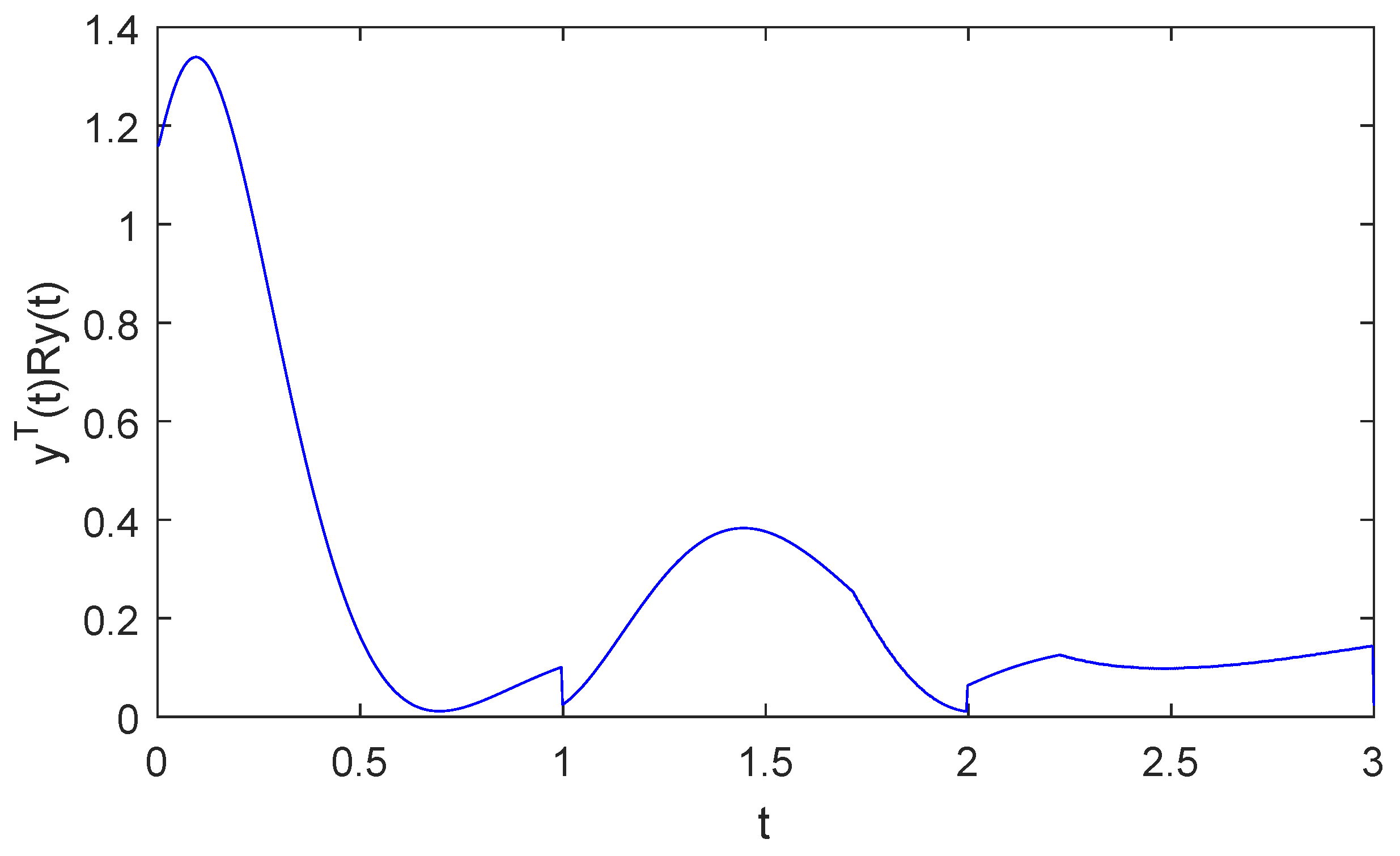
With the initial states defined as $x\left(0\right)={[1-0.6]}^T$ and an average dwell time of $\tau =1$, the simulation outcomes are shown in Figure 1, Figure 2 and Figure 3. Figure 1 demonstrates that the state trajectories of the open-loop switched systems exceed the threshold of $c=3$, indicating that the uncontrolled system is divergent. Based on Equation (25), we select an average dwell time ${\tau }_a=1.5$. Utilizing the proposed switched signal $\sigma \left(t\right)$ and SMC law $u\left(t\right)$, Figure 2 clearly demonstrates that the trajectory of $y^T\left(t\right)Ry\left(t\right)$ within the finite-time interval $[0,T]$ for the closed-loop switched system remains below the threshold value of $c=3$. Consequently, when the final time is reached, the state trajectories of the controlled switched systems are still bounded within the predefined threshold c. 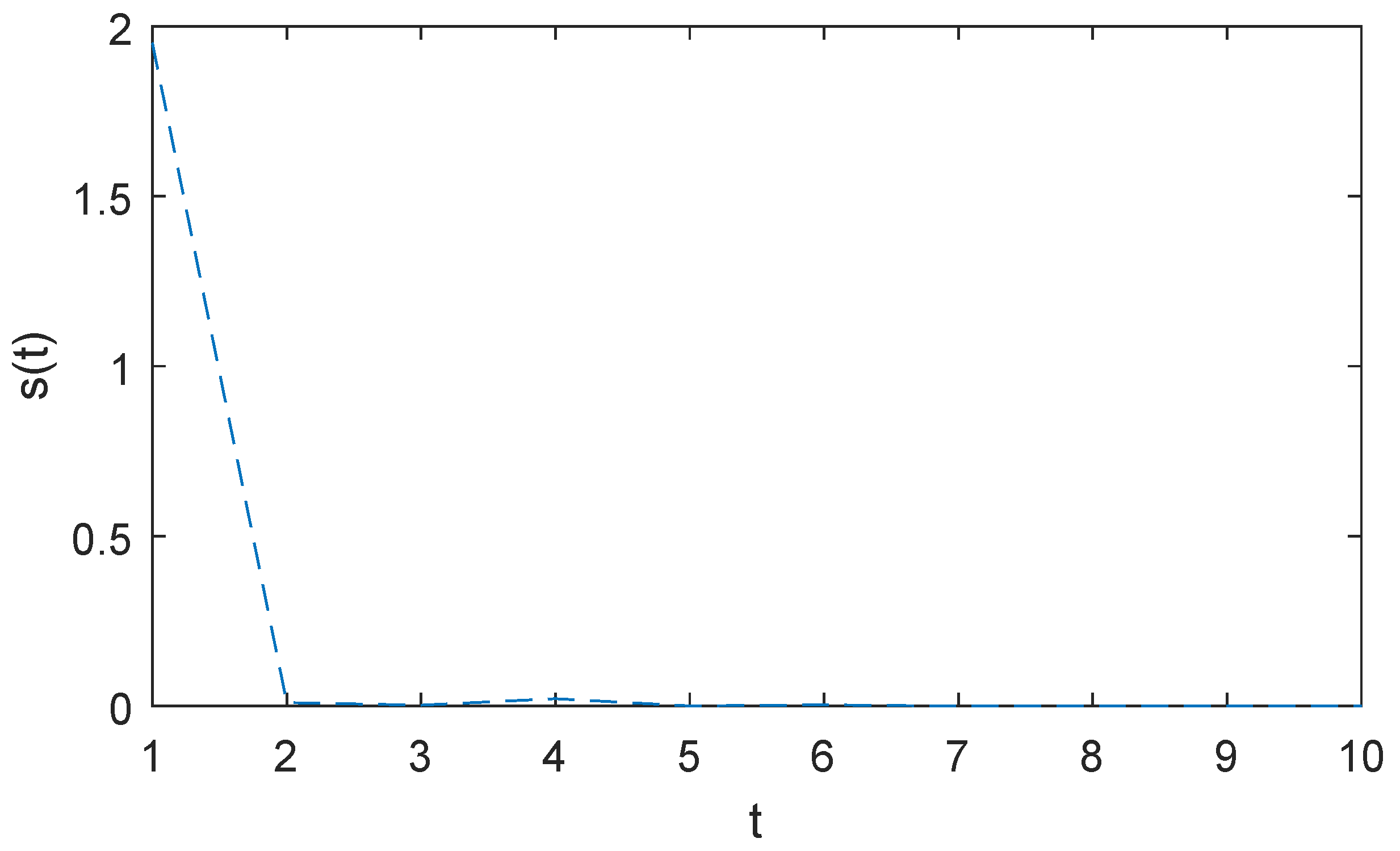Figure 3 depicts the response of the sliding variable $s\left(t\right)$.

7. Conclusions

In this research, we addressed the challenge of SMC for a class of uncertain switched systems subjected to asynchronous switching and finite-time constraints. To guarantee IO-FTS of these switched systems, a SMC controller with adjustable parameters is constructed. This controller is designed to guide the system’s state trajectory to reach the sliding surface within a predefined time interval. By applying a partitioning strategy and the MLF approach, we established sufficient conditions to ensure IO-FTS of the closed-loop switched system throughout the entire time interval $[0,T]$. In future work, we can consider incorporating adaptive control techniques, such as those demonstrated in [26,27], to enhance the intelligence of sliding mode control and reduce the conservatism of control law.

References

1. Long, L.; Zhao, J. Robust stabilisation of non-triangular multi-input switched non-linear systems and its application to a continuously stirred tank reactor system. IET Control Theory Appl. 2013, 7, 697–706. [Google Scholar] [CrossRef]
2. Wu, X.; Lin, J.; Zhang, K.; Cheng, M. A penalty function-based random search algorithm for optimal control of switched systems with stochastic constraints and its application in automobile test-driving with gear shifts. Nonlinear Anal. Hybrid Syst. 2022, 45, 101218. [Google Scholar] [CrossRef]
3. Liberzon, D.; Morse, A.S. Basic problems in stability and design of switched systems. IEEE Control Syst. Mag. 1999, 19, 59–70. [Google Scholar]
4. Li, Z.; Soh, C.B.; Xu, X. Lyapunov stability of a class of hybrid dynamic systems. Automatica 2000, 36, 297–302. [Google Scholar] [CrossRef]
5. Daafouz, J.; Riedinger, P.; Iung, C. Stability analysis and control synthesis for switched systems: A switched Lyapunov function approach. IEEE Trans. Autom. Control 2002, 47, 1883–1887. [Google Scholar] [CrossRef]
6. Zhao, X.; Zhang, L.; Shi, P.; Liu, M. Stability and stabilization of switched linear systems with mode-dependent average dwell time. IEEE Trans. Autom. Control 2011, 57, 1809–1815. [Google Scholar] [CrossRef]
7. San Filippo, F.A.; Dorato, P. Short-time parameter optimization with flight control application. Automatica 1974, 10, 425–430. [Google Scholar] [CrossRef]
8. Ou, M.; Du, H.; Li, S. Finite-time tracking control of multiple nonholonomic mobile robots. J. Frankl. Inst. 2012, 349, 2834–2860. [Google Scholar] [CrossRef]
9. Dorato, P. Short-Time Stability in Linear Time-Varying Systems; Polytechnic Institute of Brooklyn: New York City, NU, USA, 1961. [Google Scholar]
10. Guo, Y.; Yao, Y.; Wang, S.; Ma, K.; Liu, K.; Guo, J. Input–output finite-time stabilization of linear systems with finite-time boundedness. ISA Trans. 2014, 53, 977–982. [Google Scholar] [CrossRef]
11. Amato, F.; Ambrosino, R.; Cosentino, C.; De Tommasi, G. Input–output finite time stabilization of linear systems. Automatica 2010, 46, 1558–1562. [Google Scholar] [CrossRef]
12. Li, M.; Sun, L.; Yang, R. Finite-time H control for a class of discrete-time nonlinear singular systems. J. Frankl. Inst. 2018, 355, 5384–5393. [Google Scholar] [CrossRef]
13. Long, S.; Zhou, L.; Zhong, S.; Liao, D. An improved result for the finite-time stability of the singular system with time delay. J. Frankl. Inst. 2022, 359, 9006–9021. [Google Scholar] [CrossRef]
14. Kaviarasan, B.; Kwon, O.M.; Park, M.J.; Sakthivel, R. Input–output finite-time stabilization of T–S fuzzy systems through quantized control strategy. IEEE Trans. Fuzzy Syst. 2021, 30, 3589–3600. [Google Scholar] [CrossRef]
15. Shi, P.; Li, X.; Zhang, Y.; Yan, J. Event-triggered quantized input-output finite-time synchronization of Markovian neural networks. IEEE Trans. Circuits Syst. I Regul. Pap. 2022, 70, 1381–1391. [Google Scholar] [CrossRef]
16. Liu, L.; Cao, X.; Fu, Z.; Song, S. Input-output finite-time control of positive switched systems with time-varying and distributed delays. J. Control Sci. Eng. 2017, 2017, 4896764. [Google Scholar] [CrossRef]
17. Feng, T.; Wu, B.; Wang, Y.E.; Chen, Y. Input-output finite-time stability of switched singular continuous-time systems. Int. J. Control Autom. Syst. 2021, 19, 1828–1835. [Google Scholar] [CrossRef]
18. Yu, Q.; Xue, N. Input-output finite-time stability of fractional-order switched singular systems with D-perturbation. Fractal Fract. 2023, 7, 341. [Google Scholar] [CrossRef]
19. Wang, R.; Xing, J.; Xiang, Z. Finite-time asynchronous control of linear time-varying switched systems. Int. J. Adapt. Control Signal Process. 2021, 35, 1824–1841. [Google Scholar] [CrossRef]
20. Wu, Z.; Chen, W.; Fei, Z.; Liu, K.Z. Finite-time state zonotopes design for asynchronously switched systems with application to a switched converter. IEEE Trans. Circuits Syst. I Regul. Pap. 2023, 70, 4137–4145. [Google Scholar] [CrossRef]
21. Su, X.; Liu, X.; Shi, P.; Yang, R. Sliding mode control of discrete-time switched systems with repeated scalar nonlinearities. IEEE Trans. Autom. Control 2016, 62, 4604–4610. [Google Scholar] [CrossRef]
22. Lian, J.; Li, C. Event-triggered sliding mode control of uncertain switched systems via hybrid quantized feedback. IEEE Trans. Autom. Control 2020, 66, 2809–2816. [Google Scholar] [CrossRef]
23. Zhao, H.; Niu, Y.; Jia, T. Security control of cyber-physical switched systems under round-robin protocol: Input-to-state stability in probability. Inf. Sci. 2020, 508, 121–134. [Google Scholar] [CrossRef]
24. Wang, J.; Yang, Y.; Xia, J.; Shi, K.; Shen, H. Coding-decoding-based sliding mode control for networked persistent dwell-time switched systems. Int. J. Robust Nonlinear Control 2021, 31, 6055–6068. [Google Scholar] [CrossRef]
25. Zhao, H.; Niu, Y.; Song, J. Finite-time output feedback control of uncertain switched systems via sliding mode design. Int. J. Syst. Sci. 2018, 49, 984–996. [Google Scholar] [CrossRef]
26. Zhou, X.; Wang, Z.; Shen, H.; Wang, J. Systematic synthesis of a class of smooth parameter projection operators for stable adaptive systems. ASME Lett. Dyn. Syst. Control 2022, 2, 031009. [Google Scholar] [CrossRef]
27. Akella, M.R.; Subbarao, K. A novel parameter projection mechanism for smooth and stable adaptive control. Syst. Control Lett. 2005, 54, 43–51. [Google Scholar] [CrossRef]
Figure 1. Evolution of x ( t ) in an open-loop case.
Electronics 12 04519 g001
Figure 2. Evolution of y T ( t ) R y ( t ) in a closed-loop case.
Electronics 12 04519 g002
Figure 3. Sliding variable s ( t ) .
Electronics 12 04519 g003
Disclaimer/Publisher’s Note: The statements, opinions and data contained in all publications are solely those of the individual author(s) and contributor(s) and not of MDPI and/or the editor(s). MDPI and/or the editor(s) disclaim responsibility for any injury to people or property resulting from any ideas, methods, instructions or products referred to in the content.