Abstract
Over the past few decades, advances in satellite and aerial imaging technology have made it possible to acquire high-quality remote sensing images. As one of the most popular research directions of computer vision, remote sensing object detection is widely researched due to the wide application in military and civil fields. The algorithms based on convolutional neural network have made great achievements in the field of object detection. However, plenty of small and densely distributed remote sensing objects against complex background pose some challenges to object detection. In this work, an efficient anchor-free based remote sensing object detector based on YOLO (You Only Look Once) is constructed. Firstly, the backbone network is simplified for the high efficiency of detection. In order to extract the features of densely distributed objects effectively, the detection scales are adjusted based on the backbone network. Secondly, aiming at the shortcomings of CBAM, the improved CJAM (Coordinate Joint Attention Mechanism) is proposed to deal with object detection under complex background. In addition, feature enhancement modules DPFE (Dual Path Feature Enhancement) and IRFE (Inception-ResNet-Feature Enhancement) as well as PRes2Net (Parallel Res2Net) are proposed. We combine CJAM with the above modules to create DC-CSP_n, CSP-CJAM-IRFE, and CJAM-PRes2Net for better feature extraction. Thirdly, a lightweight auxiliary network is constructed to integrate the low-level and intermediate information extracted from remote sensing images into the high-level semantic information of the backbone network. The auxiliary network allows the detector to locate the target efficiently. Fourthly, Swin Transformer is introduced into the ‘Neck’ part of the network so that the network can effectively grasp the global information. The mAP on DOTA1.5 and VEDAI datasets, which both contain a large number of small objects, reached 77.07% and 63.83%, respectively. Compared with advanced algorithms such as YOLO V4, YOLO V5s, YOLO V5l, and YOLO V7, our approach achieves the highest mAP.
1. Introduction
In contrast to object recognition, it is necessary for object detection not only to determine the types of the objects but also to obtain the coordinates of the objects. So, object detection is more complex and challenging. From the whole point of view, the tasks of object detection can be seen as the fusion of object location and object recognition. In traditional object detection tasks, the mainstream approaches are usually as follows:
(1) Searching for regions of interest (ROIs);
(2) Extracting the features of ROIs;
(3) Transmitting the features to the classifiers.
Although the models of handcrafted feature design have obtained good results in object detection, there is an insurmountable bottleneck in accuracy. Within the last decade, the rapid advancement of deep convolutional neural networks (DCNN) [1,2,3,4,5,6] has revolutionized object detection. The whole new computing model and increase in computational power have made CNN-based object detection feasible.
As a significant milestone of CNN, the introduction of region-based CNN (R-CNN) [7] marked a pivotal breakthrough in the field of object detectors. Subsequently, a plethora of CNN-based object detection models have emerged, reflecting the rapid and prolific growth in this field. The approaches represented by R-CNN are called two-stage algorithms since their detection procedures contain two steps: (1) acquire regions of interest; (2) calculate the category and position of each bounding box. Based on the fundamentals of R-CNN, researchers have proposed a number of improved models such as Fast R-CNN [8], Faster R-CNN [9], Mask R-CNN [10], etc. The other main type of frameworks are called one-stage algorithms, represented by YOLO (You Look Only Once) series such as YOLO V1–V6 [11,12,13,14,15,16] as well as SSD series such as SSD [17], DSSD [18], and FSSD [19]. Usually, two-stage algorithms pay more attention to accuracy while one-stage algorithms focus on the detection efficiency.
Remote sensing object detection is widely used in military, navigation, location, and tracking of vehicles and vessels, etc. Due to the huge amount of images and the variety of objects in remote sensing images, the introduction of CNN is necessary and preferred. Unfortunately, there are big differences between traditional object detection and remote sensing object detection. Upon investigation, it becomes apparent that the sizes of remote sensing objects are highly varied, setting them apart from conventional objects. The angles and heights of the imaging equipment as well as the light conditions of the scenes vary greatly compared to conventional objects. Specifically, according to a number of studies, remote sensing object detection usually faces the following problems:
(1) Scale diversity: In remote sensing images, there are usually multi-scale objects, and the diversity of scales is not only reflected in different categories of objects, but also in the same category of objects. Aiming at this problem, the current research direction is feature fusion.
Li et al. [20] improved the R(3)Det by using the feature pyramid network to further enrich the feature information of multi-scale objects. The improved algorithm is robust for complex backgrounds, but the backbone network creates difficulties in extracting deep semantic information. In view of this defect, Zhang et al. [21] realized the fusion of multi-scale information through attention network, which enhanced the ability to extract deep semantic information. However, the redundancy of the structure is high, and it is not easy to implement. Teng et al. [22] used a simplified network to encode and design an adaptive anchor to deal with scale changes of objects in remote sensing images. This method can effectively extract semantic information, but it is difficult to deal with rotating object detection.
(2) Distribution density: Due to the wide coverage of remote sensing images, some objects are in a state of dense distribution, which makes it difficult for a feature extraction network to distinguish different objects. In response to this problem, researchers have focused on feature enhancement.
Zhou et al. [23] used the backbone network of CSP structure to achieve high-precision detection. Although the algorithm has a high accuracy, the mAP is still lower than expected when facing some small objects. Hou et al. [24] enhanced the feature extraction of the network by CBAM, and the use of attention mechanism improves the feature extraction capability of the network. However, the detection performance is still insufficient when facing small objects.
(3) Shape diversity: The object in optical remote sensing image is also reflected in the shape diversity, that is, the shape of the object in different categories is often very different. To solve this problem, the prevailing approaches are to improve the anchor and network.
The improvement strategy of anchor is usually to increase the number and categories of anchor boxes [25,26,27,28]. However, the effect is not obvious.
In the aspect of network improvement, deformable convolution stands as a significant breakthrough. Xu et al. [29] used a backbone network consisting almost entirely of deformable convolution to detect multi-shaped objects. Ren et al. [30] improved Faster RCNN by deformable convolution. Deformable convolution is not satisfactory for performance improvement and increases the complexity of network.
(4) Background complexity: Due to its wide coverage, remote sensing images contain a large number of objects of various categories, while the marked object categories to be detected are relatively small. As a result, the background accounts for most of the entire image area. Remote sensing objects are often surrounded by a complex background. Researchers often address this problem by enhancing object features while weakening the background information.
Wang et al. [31] proposed an improved cascade algorithm to accurately locate remote sensing objects. Cheng et al. [32] proposed a CNN-base diversified context information fusion algorithm to improve the detection accuracy under a complex background.
Although a series of algorithms have been proposed for remote sensing object detection, their performance is still not satisfactory. In this paper, an efficient remote sensing object detector with an anchor-free mechanism is proposed to achieve the balance between high-precision detection and real-time detection. The contributions of this paper are as follows:
(1) In order to reduce the computing load of the network, a lightweight network is proposed in this paper.
(2) Aiming at the difficulty of feature extraction of densely distributed remote sensing objects, the detection scales are adjusted on the basis of lightweight network. The detection scales are expanded so that the network can effectively separate the features of densely distributed objects.
(3) In order to improve the overall performance of the network for remote sensing object detection under complex background, a new attention mechanism called CJAM is proposed based on CBAM.
(4) In addition, the feature enhancement modules DPFE and IRFE are proposed to improve the feature extraction capability of the network and make the network adapt to the detection of multi-shaped objects.
(5) In order to improve the overall receptive field of the network, an improved PRes2Net is proposed to replace the SPP in YOLO V4.
(6) In order to improve the sensitivity of the network to global information, Swin Transformer is integrated into the ‘Neck’ part of the network.
(7) In order to enhance the localization of an object, a small auxiliary network is proposed to realize the fusion of different levels of feature information.
The remainder of this paper is organized as follows: Section 2 introduces the principle and development of YOLO. Section 3 describes the methodology of our approach. Section 4 exhibits the experimental results. Section 5 presents the discussion. Finally, Section 6 provides the conclusion and prospects for future work.
2. The Proposal and Development of YOLO
Similar to as SSD, YOLO is a typical one-stage detector that does not have the process of region proposal. In contrast to two-stage detectors, YOLO treats the process of target detection as a regression problem. The core idea of YOLO is to feed the entire image into the network and acquire the location and classification information of the targets directly. The output of YOLO is the tensor containing the location, classification information, and confidence score. Therefore, it can detect multiple targets. Since the framework and the process of detection is concise, it gains faster detection speed. However, the number of the output grid cells is limited to . YOLO has poor performance on small target detection. In addition, only one target can be detected by one grid cell, YOLO does not have the ability to deal with densely contributed targets.
To solve these problems, the improved version YOLO-V2 was proposed. YOLO-V2 adopts a series of measures: (1) it YOLO-V2 improves the accuracy by introducing BN (Batch Normalization). (2) The size of the input is replaced from to . (3) The concept of the anchor box is adopted. With these adopted measures, the performance of YOLO-V2 is distinctly improved.
The performance of YOLO-V2 for detecting small targets especially densely distribution small targets, still has drawbacks that are unsatisfactory. Therefore, YOLO-V3 was proposed, based on YOLO-V2. The most important improvements are as follows: (1) YOLO-V3 adopts FPN (Feature Pyramid Network) to predict bounding boxes at three scales. (2) A brand new deep convolutional neural network named Darknet 53 was adopted as the backbone network of YOLO-V3. As its name implies, it contains 53 layers. Darknet53 adopts successive and convolutional kernel and uses skip connections, inspired by ResNet. YOLO-V3 obtains a clear advantage compared to YOLO-V2 in detecting small targets.
Based on YOLO V3, more advanced versions such as YOLO V4–V6 have been successively proposed. As a type of classic target detection model, YOLO shows good performance in speed and accuracy.
3. Materials and Methods
Although YOLO-V4 has achieved great achievements on object detection, there are still limitations regarding specific tasks. In remote sensing images, a complex environment often results in lower detection accuracy. In addition, dense distribution and illumination interference will also affect the performance of object detection. In this paper, we aim to realize three objectives: (1) To improve the accuracy in detecting remote sensing objects, surpassing the performance of existing state-of-the-art detectors. (2) To effectively detect densely distributed objects and small objects under complex background. (3) Finally, to consider both accuracy and detection speed.
3.1. The Lightweight Feature Extraction Network
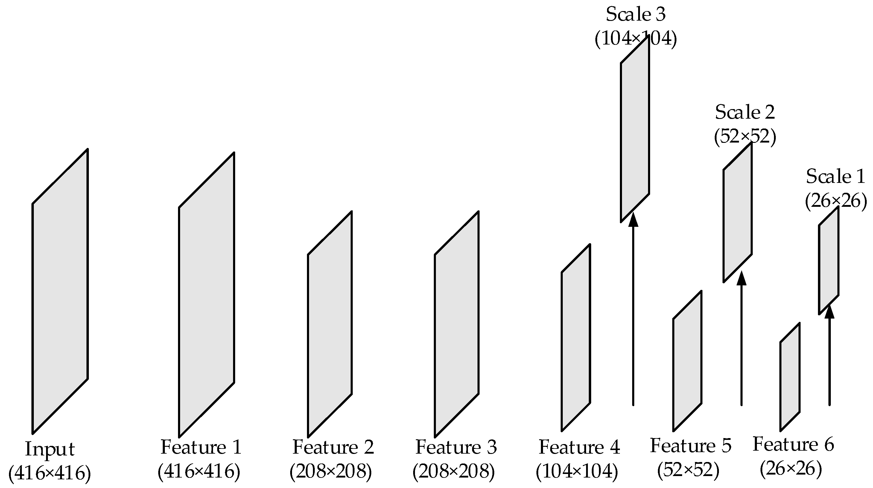
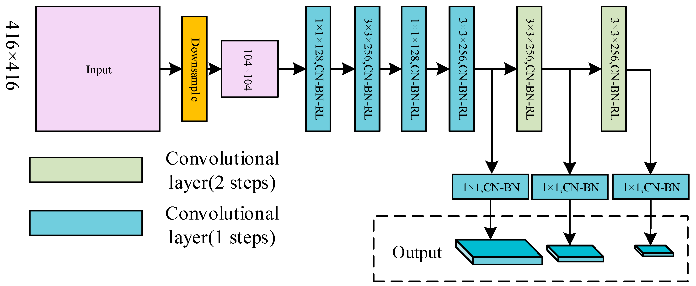
The structure of CSPDarkNet53 employed by YOLO-V4 is concise. However, CSPDarkNet53 has its inherent disadvantages in detecting very small objects or densely distributed objects. There are 3 detection scales in the network. If the input size is , the sizes of the detection scales will be , , and , respectively. That is to say, the features of the 3 detection scales are down sampled by , and , respectively. So, the size of the objects that can be detected is limited. After being down sampled by , the size of the object feature that is less than will take up less than 1 pixel, and the object will not be detected effectively. Similarly, if the center distance between the 2 objects is less than 8 pixels, the features of them will be located in 1 grid cell. The defects mentioned above make it difficult for the network to detect very small and densely distributed objects. Although the existing YOLO models enhance the performance of object detection, they still exhibit limitations in detecting small-sized, densely distributed remote sensing objects. For the backbone networks of the existing YOLO models, high-sampling feature maps will lead to network redundancy, which is unnecessary. In this section, the convolutional layers of size are removed. Then, the sizes of the detection layers after streamlining the structure of backbone network are changed from , , and to , , and . The streamlined network can effectively separate the features of small and densely distributed objects. The simplified transitional backbone network is shown in Figure 1.
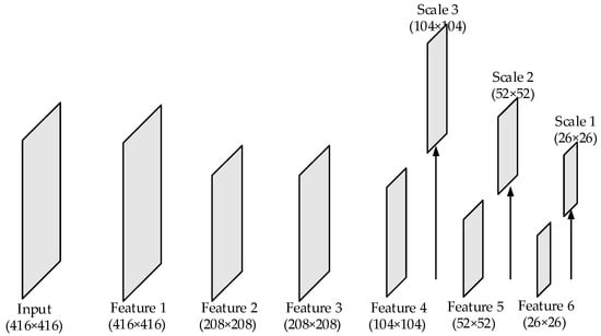
Figure 1.
The structure of transitional backbone network. The arrows point to three detection scales: Scale 1, Scale 2, and Scale 3. Their sizes are 26 × 26, 52 × 52, and 104 × 104, respectively.
3.2. Coordinate Joint Attention Mechanism
Remote sensing images often contain complex backgrounds. In order to address this problem, we consider introducing attention mechanism [33,34,35,36] into the feature extraction network to suppress background information and strengthen object feature information.
When the human eye encounters a scene, it quickly focuses on certain areas of the scene after a quick search to make timely and accurate response measures. This mechanism is referred to as the visual attention mechanism.
Researchers have proposed the idea of visual attention mechanism in deep learning by drawing on the feature of human intuition. The attention mechanism simulates the uneven distribution of human eye attention. By weighting the coding information, more valuable computing resources are allocated in a biased way to obtain more useful coding information. When training the network, the distribution of weights is constantly changing in the direction that the loss function decreases. The network learns the importance of different information until it converges and finally completes the object detection task.
So far, the attention mechanism models adopted by a large number of networks are the channel attention mechanism represented by SENet [37], ECA [38], and CBMA [39] or their improved models. SENet and ECA calculate the attention between channels by two-dimensional global pooling and achieve good results at a relatively low computational cost. However, the channel attention mechanism only takes into account the information between coded channels and ignores the importance of location information. The CBAM attempts to mine location information by reducing the channel dimension of the input tensor and then calculates spatial attention using convolution. However, it only obtains the local relation of the location and cannot model the remote dependence, which is important for object detection.
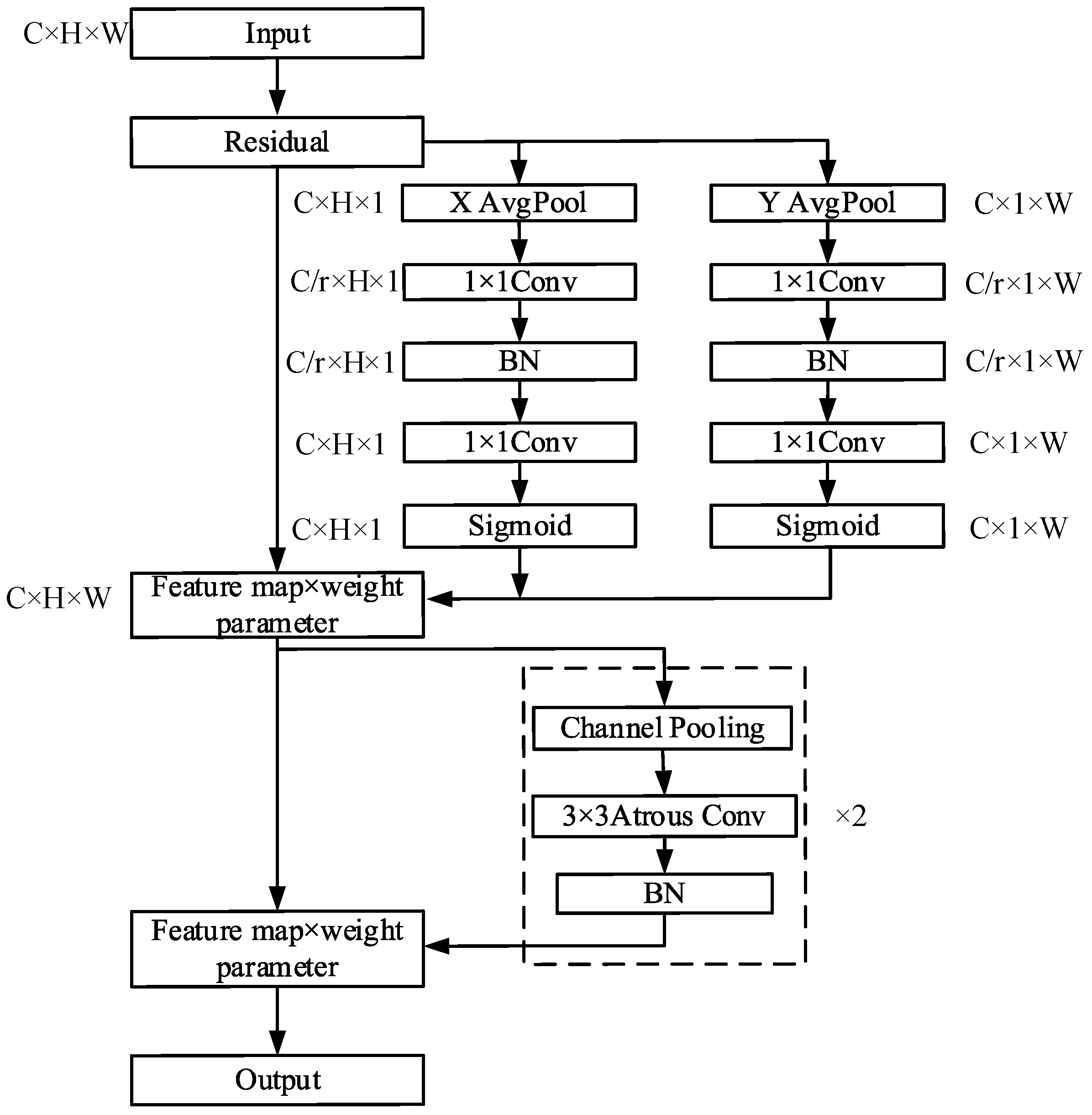
To overcome the shortcomings of CBAM, a new attention mechanism model is proposed. By incorporating local information into CBAM, it can mitigate local information loss caused by 2D global pooling. In the newly proposed attention mechanism, the channel attention mechanism is divided into 1D pooling processes to effectively integrate spatial coordinate information into the attention mappings. The proposed attention mechanism is called coordinate joint attention mechanism (CJAM) and the structure is shown in Figure 2.
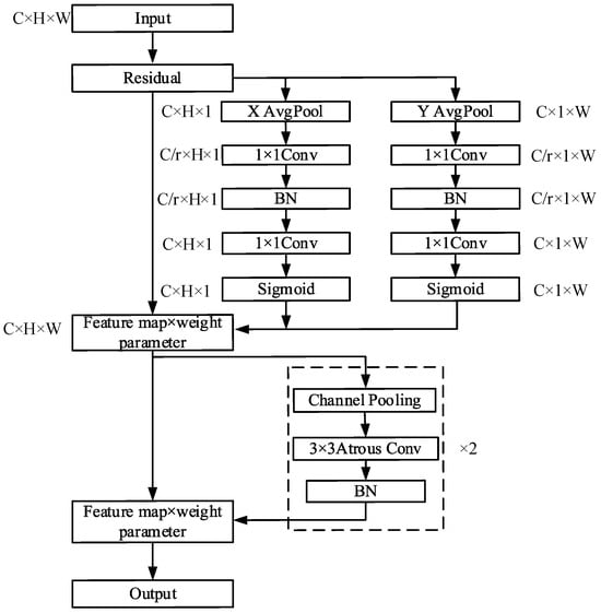
Figure 2.
The structure of CJAM.
To be specific, in order to convert the input feature mappings into a vertical direction and horizontal direction, 1D global average pooling is adopted. After that, two feature mappings with directional information are decoded into two attention maps by two 1 × 1 convolution kernels. Each attention map can capture the long distant dependencies along a particular direction in the feature map. Thus, the coordinate information can be saved.
In the channel attention mechanism, global pooling compresses global spatial information into channel information. This makes location information difficult to retain, which will adversely affect the acquisition of object location information in object detection tasks. Therefore, we decompose global pooling into the vertical and horizontal mappings mentioned above. Each channel is encoded by two kernels: and . For input , the output of channel, where the height is , can be shown in Equation (1).
Similarly, the output of the channel, where the width is , can be shown in Equation (2).
The above two equations generate direction-aware feature mappings in different directions. This allows the attentional mechanism model to acquire long distant dependencies when it goes along a particular direction while reserving precise location information in the other direction. Then, similar to the SE attention mechanism and CBAM attention mechanism, CJAM also performs the squeeze and excitation steps on the channels. The difference is that CJAM eliminates the full connection layer and adopts two 1 × 1 convolutions, respectively, for channel compression. Then the channels are expanded by two 1 × 1 convolutions, respectively, and the obtained weight parameters are multiplied with the feature graph to obtain the coordinate attention feature graph. This process can be expressed in Equations (3)–(7).
In Equations (3) and (4), and represent the transformation function of 1 × 1 convolution. represents activation function ReLU. and represent the horizontal and vertical eigenvectors of encoding spatial information acquisition. In Equations (5) and (6), and represent the transformation function of 1 × 1 convolution. represents activation function Sigmoid. and are the same tensor as the number of input channels obtained after two convolution and activation functions. In Equation (7), the input and the two tensors , are multiplied together to get the output of the coordinate attention mechanism.
In addition, CJAM also incorporates the spatial attention mechanism. By multiplying the matrix obtained through the spatial attention mechanism and the output, the final output of CJAM can be expressed as:
In Equation (8), Avg and Max represent the average and maximum pooling, respectively. represents the addition of the corresponding parameters. represents atrous convolution, where the kernel is 3 × 3 and the dilation rate is 2. represents the activation function Sigmoid.
CJAM, which is proposed in this paper, is composed of two parts: coordinate attention mechanism and spatial attention mechanism. In view of the defect that the channel attention mechanism in CBAM can only obtain local relation of position, the channel attention mechanism in CJAM is split into two parts along the horizontal and vertical directions. Through average pooling and convolution on the x and y axes, respectively, the information between different channels can be obtained effectively. Additionally, the position information is more sensitive, which is beneficial to the accurate location of the object position information in the object detection task.
3.3. DC-CSP_n Feature Enhancement Module in Backbone Network
In Section 3.1, the backbone network is simplified, and the sizes of the detection layers are adjusted. Although the transitional backbone network in Figure 2 is able to separate the features effectively, the performance of feature extraction is confined due to the smaller number of convolutional layers. Improving the performance of CNNs remains a pressing topic for researchers, and this work is no exception.
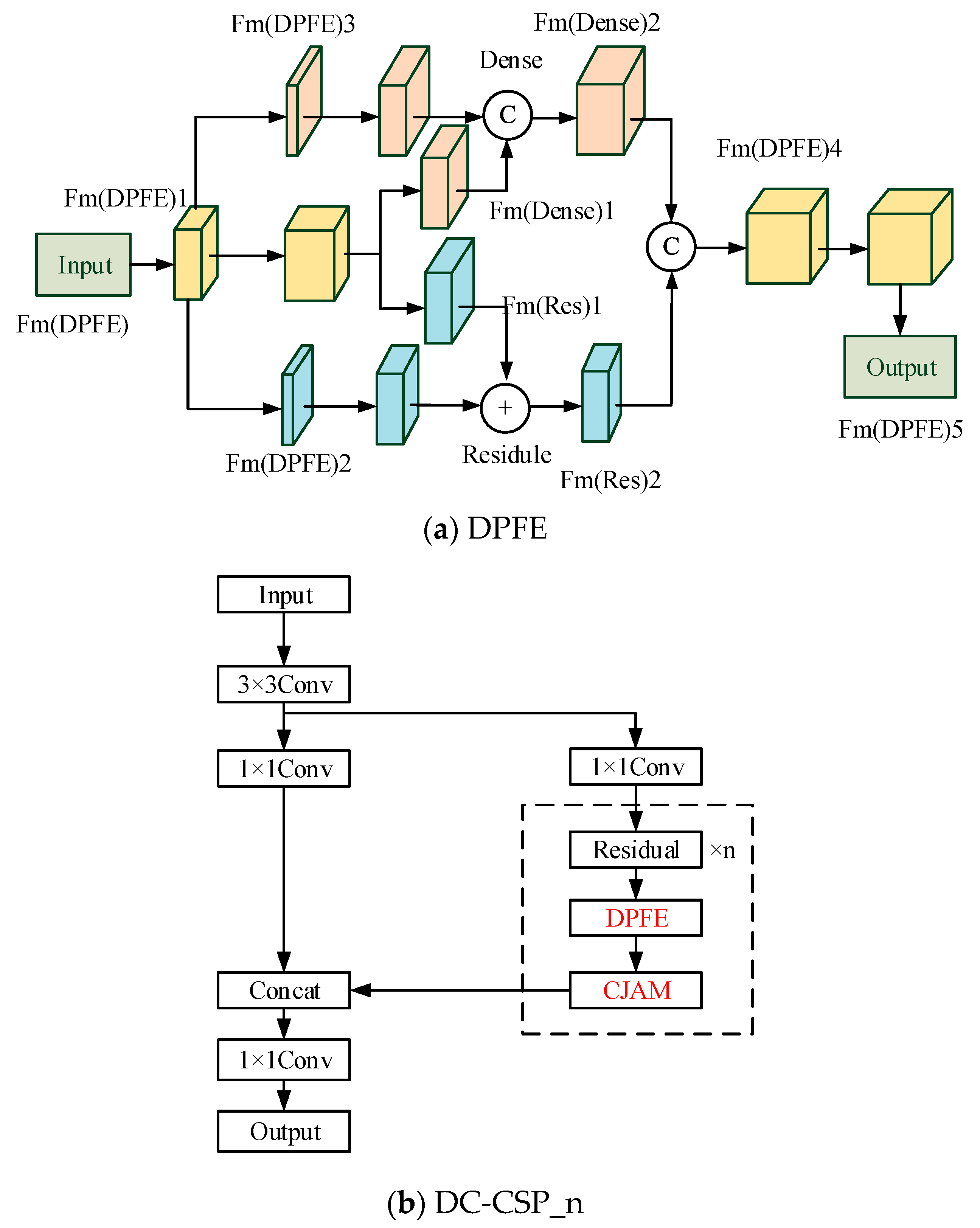
Inspired by Dual Path Network (DPN) [40], the feature enhancement module DPFE is proposed. In addition, combining CSP structure and CJAM in Section 3.2, DC-CSP_n is proposed for feature enhancement. Figure 3 exhibits the structure of DPFE and DC-CSP_n.
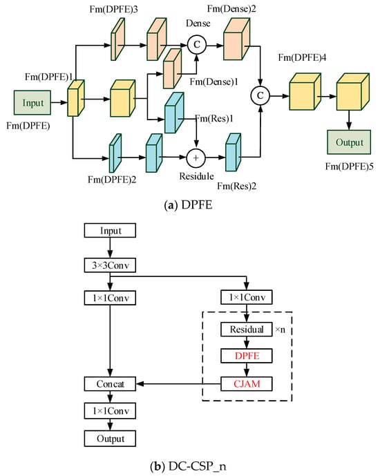
Figure 3.
The structure of DPFE and DC-CSP_n.
In Figure 3a, DPFE consists of two parts: residual structure and densely connection structure. Both parts use 1 × 1 and 3 × 3 convolution kernels. Fm(DPFE)5, Fm(DPFE)4, Fm(Res)2, and Fm(Dense)2 can be expressed as:
In Equations (9)–(12), represents the transformation function of 1 × 1 and 3 × 3 convolution. and represent the ‘Add’ and ‘Concat’ operations, respectively.
In Figure 3b, based on DPFE, the CJAM attention mechanism is integrated, and the DC-CSP_n module based on CSP structure is built to improve the performance of feature extraction.
3.4. CSP-CJAM-IRFE Feature Enhancement Module in Detection Layers
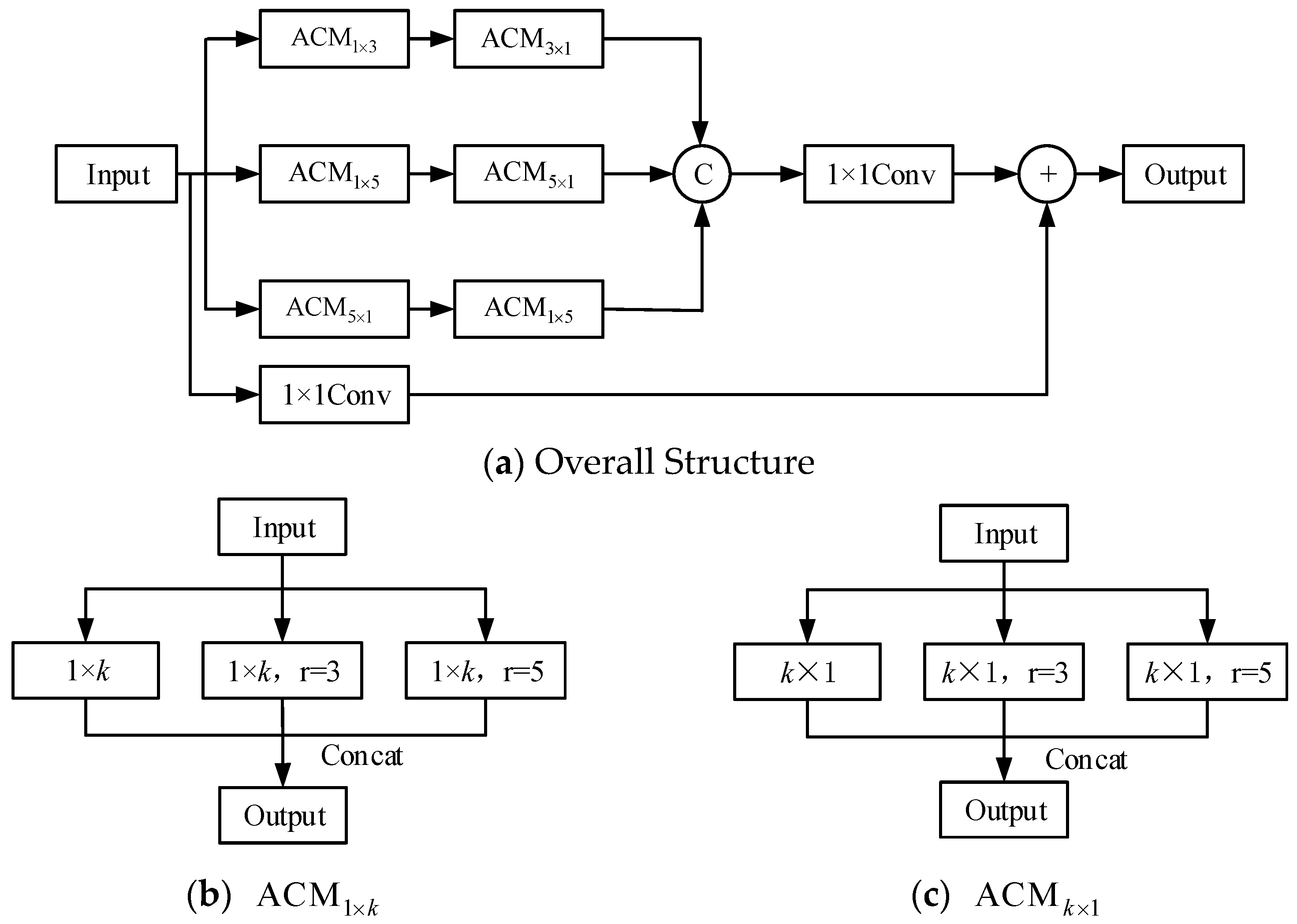
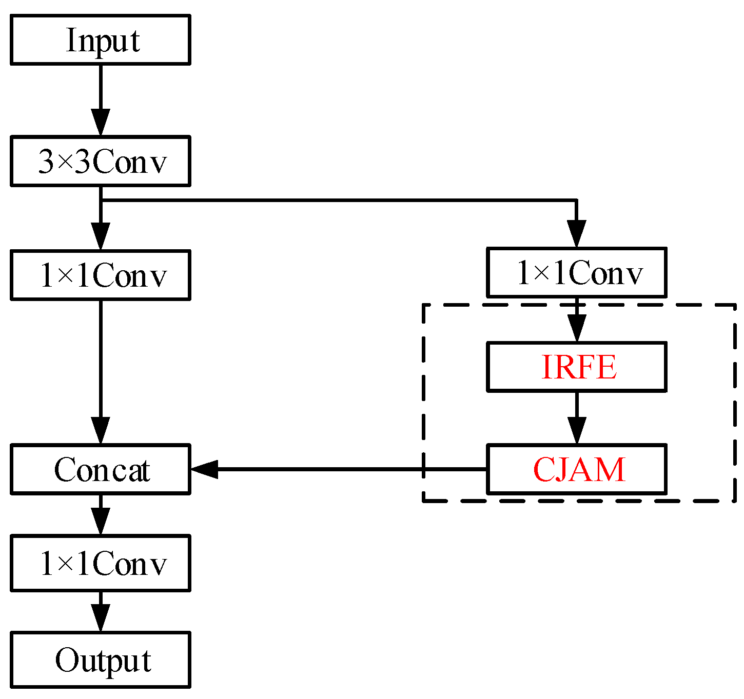
Remote sensing objects are often characterized by the diversity of shapes. For multi-shape object detection, a lot of studies focus on adding deformable convolution into the network. Due to the complexity of the calculation, deformable convolution brings some negative effects on training and parameter number control. To solve this problem, a strategy of feature extraction and fusion using convolution kernels of different sizes is adopted based on the principle of Inception [41,42,43]. For 3 × 3 and 5 × 5 convolution of size, they are split into 3 × 1 and 1 × 3 convolution as well as 5 × 1 and 1 × 5 convolution. This method greatly reduces the computation amount on the premise of constant receptive field. Adding convolution kernels of different shapes to the network can assist the network in learning the object feature information of different shapes. In addition, The Atrous Convolution Module (ACM) is proposed for the decomposition of k × k convolution kernel. We call this network integrating Inception and ResNet as IRFE (Inception-ResNet-Feature Enhancement Module). The structure is shown in Figure 4.
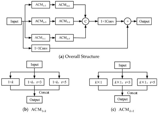
Figure 4.
The structure of IRFE.
IRFE proposed in this section adopts the method of increasing the width to improve the performance. In addition, large convolution kernels of size k × k are decomposed, and ACM is used to combine convolution kernels of different sizes. In Figure 4b, there are 3 parallel convolution operations: 1 × k convolution, 1 × k atrous convolution, where the dilation rate is 3, and 1 × k atrous convolution, where the dilation rate is 5. In Figure 4c, there are also 3 parallel convolution operations: a convolution of size k × 1, atrous convolution, where the kernel is k × 1 and the dilation rate is 3, and atrous convolution, where the kernel is k × 1 and the dilation rate is 5.
The fusion of convolution kernels of different shapes and sizes into IRFE can make the network adapt to the detection of multi-shape objects. In addition, by integrating IRFE, the CSP structure, and CJAM, CSP-CJAM-IRFE feature enhancement module is constructed, and its structure is shown in Figure 5.
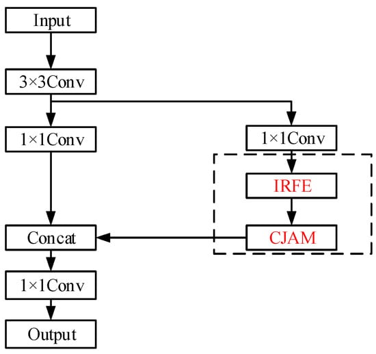
Figure 5.
The structure of CSP-CJAM-IRFE.
3.5. CJAM-PRes2Net Receptive Field Amplification Module
The backbone networks in YOLO V4 and YOLO v5 adopt SPP (Spatial Pyramid Pooling) [44] for receptive field amplification. SPP uses different convolution kernels for convolution, and then channels are spliced to enhance the receptive field. Compared to SPP, Res2Net performs better. Therefore, Res2Net will be adopted as the receptive field enhancement module in this paper.
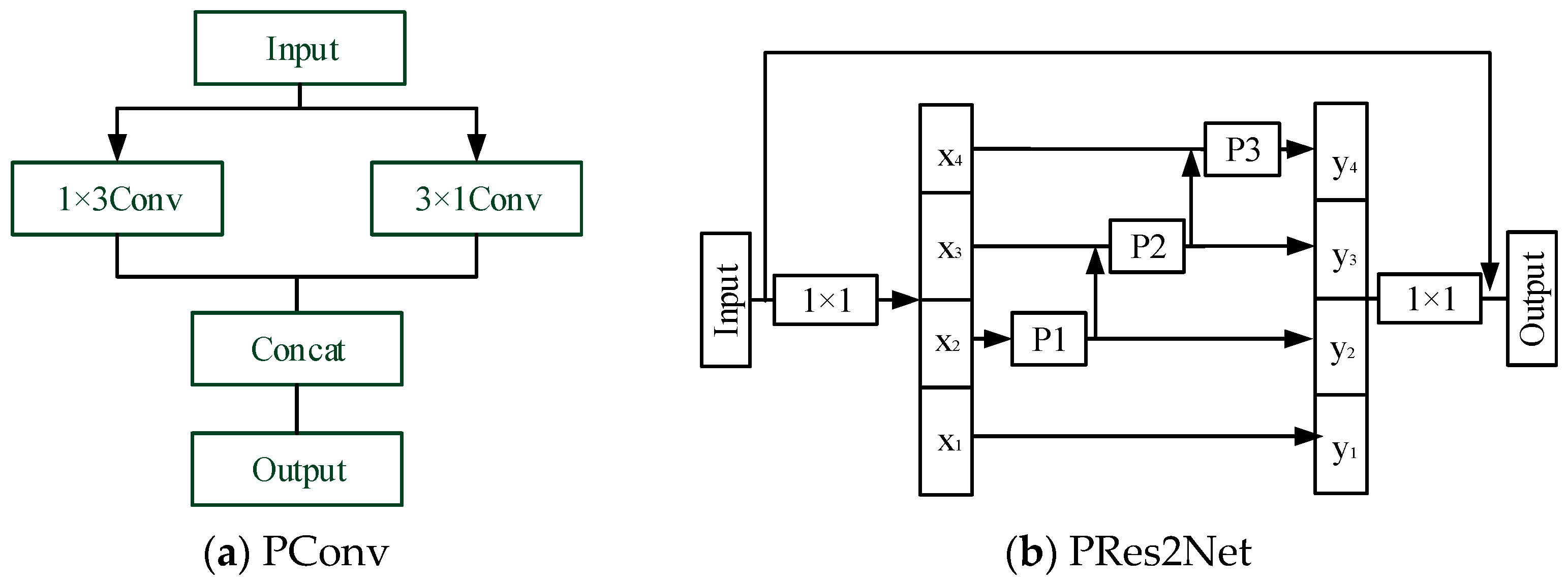
In order to reduce the computing load to a certain extent, a parallel combination of 1 × 3 and 3 × 1 convolution kernels is adopted. In this paper, Parallel Res2Net (PRes2Net) constructed by parallel convolution is used to replace the original SPP. The structure of PRes2Net is shown in Figure 6.
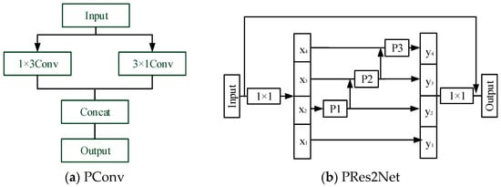
Figure 6.
The structure of PRes2Net.
In Figure 6a, parallel convolution (PConv) decomposes the 3 × 3 convolution kernel into two different shapes: 1 × 3 and 3 × 1, which not only reduces the computational load, but also obtains the same receptive field as the 3 × 3 convolution. Figure 6b shows an improved PRes2Net whose internal convolution kernels P1, P2, and P3 are parallel convolution in Figure 6a. The overall receptive field of the network is further improved by increasing the sizes of convolutional kernels, which are 3 × 3, 5 × 5, 7 × 7, respectively. In addition, we adopt the combination of 1 × k and k × 1 convolution instead of k × k convolution. The output of the internal branches of the improved PRes2Net is shown as follows.
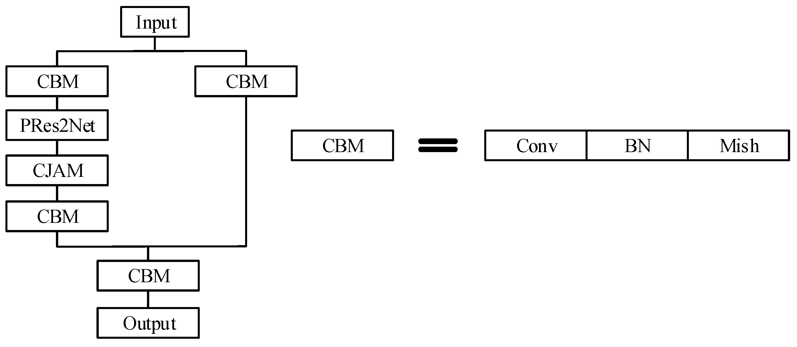
In Equation (13), represents convolution operation. represents parallel convolution kernels of size 1 × k and k × 1. We combine CJMA with the improved PRes2Net to form a residual attentional module. Figure 7 exhibits the structure of improved CJAM-Res2Net.
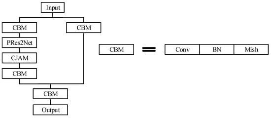
Figure 7.
CJAM-PRes2Net.
The improved CJAM-Res2Net combines PRes2Net and CJAM. First, the channel is adjusted by two CBM modules of 1 × 1 kernel and is divided into two branches. The output from the first branch is fed into PRes2Net and then into CJAM. Merging the output of the two branches and then through a CBM module of 1 × 1 kernel, the final output will be obtained. The CJAM-PRes2Net module proposed in this section can not only gradually expand the overall receptive field of the network, but also integrate the advantages of CJMA attention mechanism.
3.6. The Application of Swin Transformer Application
Transformer [45] is of great significance for object detection. Inspired by this, integrating Transformer into CNN can improve the performance of object detection. Ordinary convolution is limited by convolution kernels and cannot perceive information outside the convolution kernels. With the adopted self-attention mechanism, Transformer Encoder can perceive global information. Therefore, compared to CNN, Transformer has a better ability to capture global information. In this section, we borrow the ideas from Transformer and incorporate Swin Transformer [46] into the ‘Neck’ part of the network.
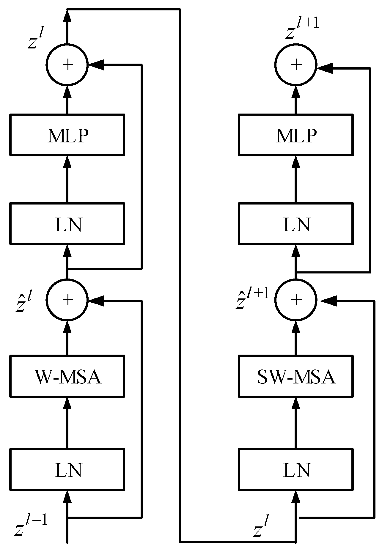
Figure 8 shows the structure of the Swin Transformer. It mainly consists of four parts, which are: LN (Layer Normalization), W-MSA (Window based Multi-head Self-Attention), SW-MSA (Shifted Window based Multi-head Self-Attention), and MLP (Multi-Layer Perceptron). LN is responsible for the normalization of information between channels. In view of the complexity of multi-head self-attention calculation in Transformer, W-MSA improves the calculation mode and uses self-attention calculation to process each window to reduce the computing load. SW-MSA improves performance by exchanging information through self-attention mechanisms between windows.

Figure 8.
The structure of the Swin Transformer.
The output of each part of the Swin Transformer can be expressed as:
In Equations (14)–(17), and refer to the output of W-MSA and SW-MSA. , , , and represent the transformation of W-MSA, MLP, LN, and SW-MSA modules, respectively.
In this section, Swin Transformer is integrated into the ‘Neck’ part of the network, and the Swin Transformer module is introduced to help the network perceive global information.
3.7. The Tiny Independent Auxiliary Network
The detection effect of existing detectors is still lower than expected when facing some small objects. In addition, most one-step detectors focus on improving the backbone networks for better performance of feature extraction. For the tasks of small object detection, low and intermediate level information is needed to describe the object information (contour, shape, etc.). Furthermore, high-level semantic information is also necessary for the separation of objects and backgrounds.
As previously discussed, when detecting multi-scale objects, low and mid-level information as well as high-level semantics information is needed. FPN fuses high-level information with high-resolution features. Despite this, this kind of top-down feature pyramid network can achieve good results in feature representation, as it only infuses high-level semantic information to the former layers. In this section, the key emphasis in work is fusing high-level information to formal layers and fusing lower and mid-level features to the later ones.
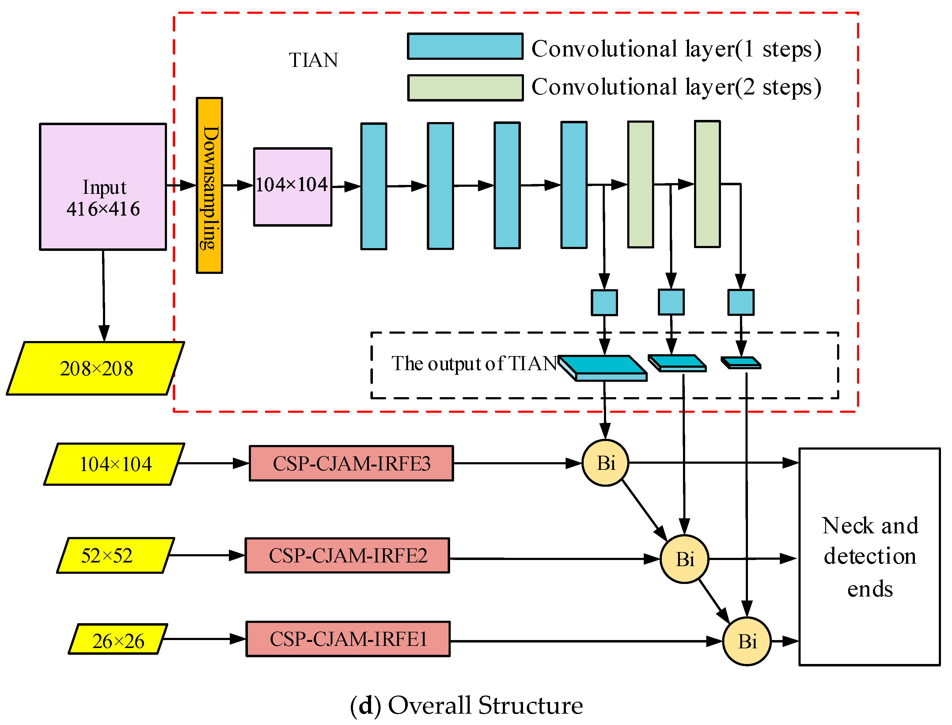
In this section, a tiny independent auxiliary network (TIAN) is built. We take the down sampled image as the input of TIAN. Then the down sampled image generates three feature maps with several convolutional layers. The three feature maps output by TIAN can effectively construct the low- and mid-level information of the image. The features are then injected into each detection layer. The structure of TIAN is shown in Figure 9 below.
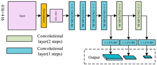
Figure 9.
The structure of TIAN.
The existing object detection framework usually adopts a deep convolutional network to produce strong semantic feature information. Semantic information is required for accurate object depict. Low- and mid-level feature information (such as outline and shape of the object) is important. In order to make up for the loss of low- and mid-level feature information from the backbone network, TIAN uses down sampling operations instead of convolutional layer for scale compression. The structure of the auxiliary network (TIAN) proposed in this section is concise. The output features of it are responsible for producing low- and mid-level information and they are then fused in the detection layers of the backbone network. Firstly, the input image is adjusted to the same size as the first detection layer by down sampling. Then the auxiliary network produces the other two scales by two convolutional layers, respectively. At last, the output features of the auxiliary are fused to the detection ends of the backbone network.
3.8. Anchor-Free Mechanism
The CNN-based algorithms for object detection can be divided into anchor-based and anchor-free algorithms. The key difference between these approaches lies in whether or not they adopt the ‘anchor box’ to extract object candidate boxes. The anchor-free mechanism is not a new concept. YOLO V1 is the earliest model to adopt the anchor-free mechanism. However, its inherent disadvantage is that each grid can only detect one object, which makes the performance of the network difficult to improve. Since version V2, YOLO has introduced the concept of anchors, continuously improving the detection accuracy. However, anchor-based algorithms need to set the anchors manually or through clustering, which makes it necessary to set the anchors with different size proportions and sizes according to the specific situation of the datasets. In addition, the operation of pre-setting many anchors makes the process time-consuming. In this section, we adopt an anchor-free mechanism for better universality of the detector.
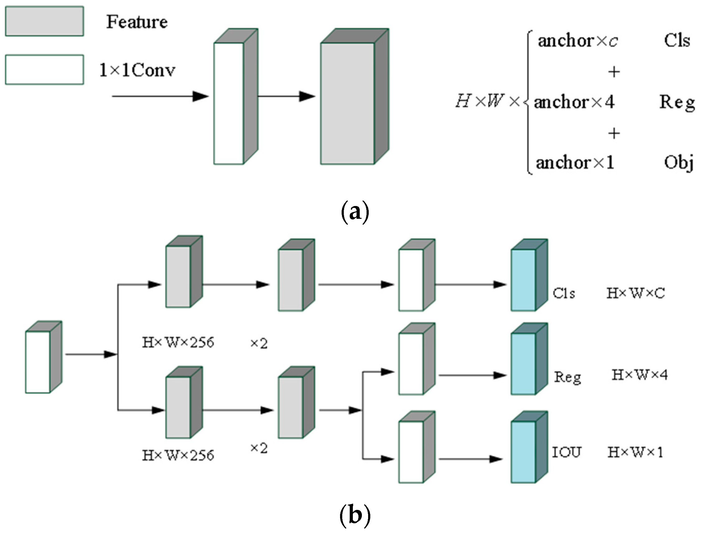
When detecting objects, many object detectors, whether one-stage or two-stage, adopt decoupling heads based on classification and positioning. During the development of YOLO, the detection end keeps coupling, and its structure is shown in Figure 10a.
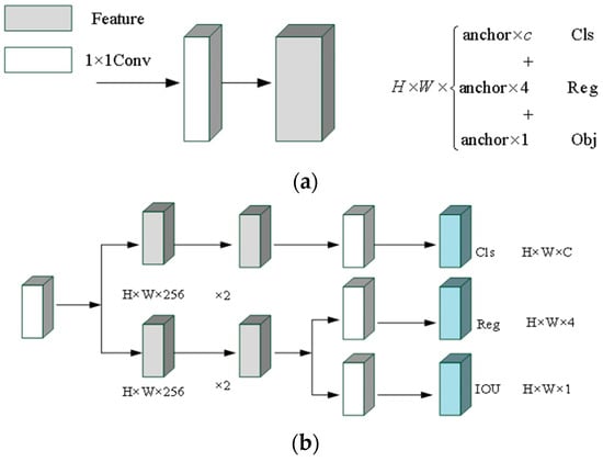
Figure 10.
The detection end of anchor-based mechanism and anchor-free mechanism. (a) Anchor-based mechanism; (b) anchor-free mechanism.
YOLO realizes the classification task and regression task with convolutional layers, which brings adverse effects to the detection and recognition of objects for the network. Inspired by the structure of detection ends of FCOS [47] and YOLOX, the anchor-free mechanism is adopted in this work. The tensor of each original detection end for the calculation of object position information and classification information are split into two parts to realize the classification task and regression task, respectively. The structure of the anchor-free detection end is shown in Figure 10b.
For each detection end, the network will predict three results. The final prediction results are , , and , respectively. In the above three prediction results, Reg is used to obtain the regression parameters for accurate location information. Obj is used to determine whether the point is included in the object. Cls is used to determine the category information of the object. After combining the three prediction results, the obtained output tensor is: . Compared with the original coupling detection end, the number of the parameters is reduced, which makes the network run faster.
3.9. Overall Framework of the Model
In this paper, BiCAM-Detector is proposed to detect densely distributed small targets under a complex background in remote sensing images. Firstly, a lightweight network is adopted, and the sizes of the detection end are adjusted to adapt to the detection of densely distributed objects. Secondly, a new coordinate joint attention mechanism, CJAM, is proposed. CJAM is integrated with DPFE and IRFE for further performance improvement. Thirdly, the internal connection structure of Res2Net is improved and combined with the CJMA module as the final output module of the backbone network, thereby expanding the receptive field of the network. Fourthly, in order to further improve network performance and enhance the network’s ability to grasp global information, Swin Transformer is adopted. Fifthly, a small independent auxiliary network is proposed to extract the low and intermediate information in the image to improve the localization ability of the network. Finally, inspired by FCOS and YOLOX, we adopt the anchor-free mechanism in the detection ends to reduce the dependence of clustering to obtain anchors from the dataset, making it more general. In Figure 11, we exhibit the backbone network and overall architecture of BiCAM-Detector.
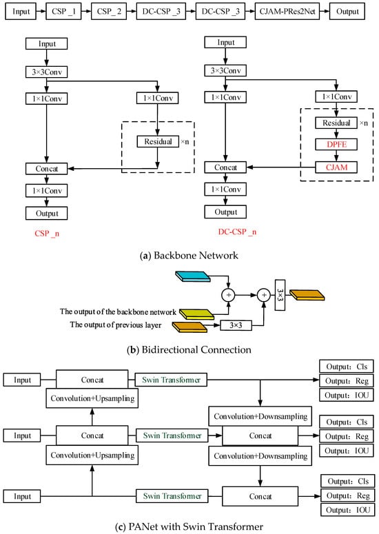
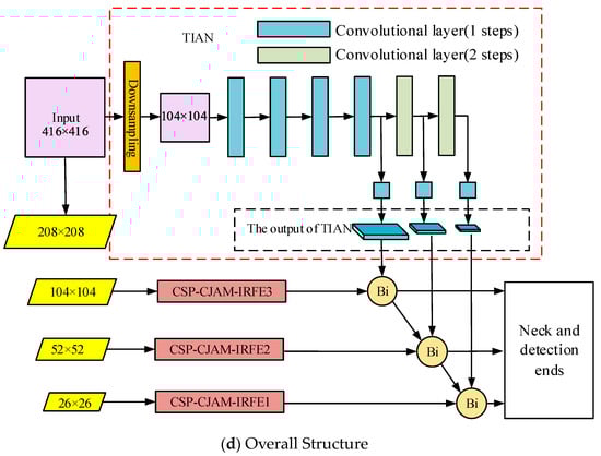
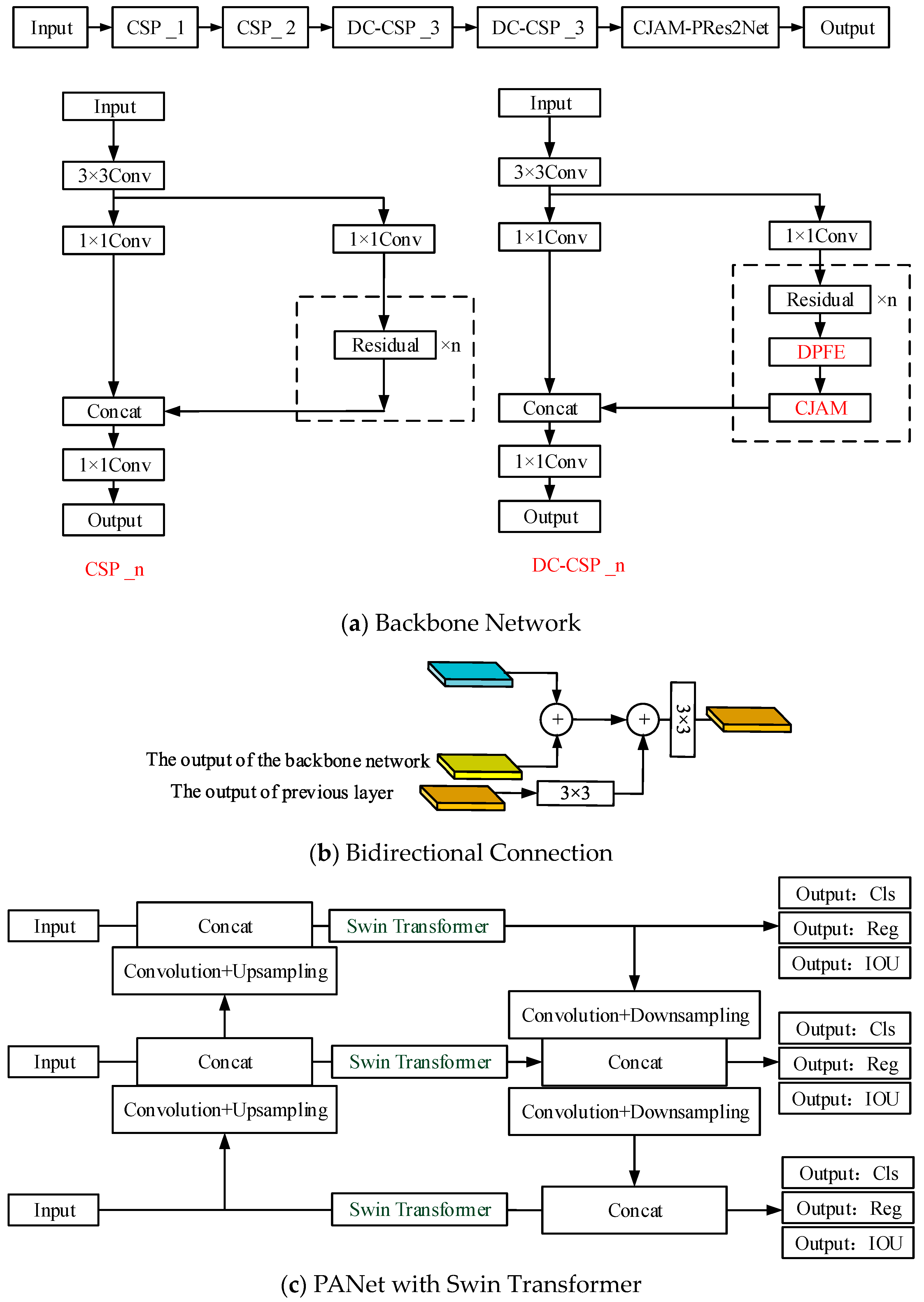
Figure 11.
The structure of the BiCAM-Detector.
Figure 11a shows the backbone network of our approach. Among them, CSP_1 and CSP_2 are residual modules with a CSP structure. DC-CSP_3 is the residual module that integrates DPFE and CJAM. Figure 11b shows the connection mode of the TIAN. First, the feature maps extracted from the backbone network are added to the outputs of TIAN. The feature map is then added with the features of the previous layer by 3 × 3 convolution transformation. Finally, the output of the current layer is obtained after 3 × 3 convolution transformation. Figure 11c shows the improved PANet, which further adds the Swin Transformer modules on the basis of the original ‘Neck’ part to improve the overall performance of the network. Figure 11d is the overall structure of our approach. It is generally composed of four parts. The backbone network is responsible for feature extraction. TIAN is responsible for the extraction of middle- and low-level features. The bidirectional connection structure is responsible for the fusion of the features from TIAN and backbone network. ‘Neck’ is responsible for the fusion of features at different levels. The detection ends are responsible for the output of the detection results.
4. Results
This section first introduces the experimental environment and datasets. Subsequently, a large number of comparative experiments are carried out on the two datasets and the proposed algorithm is compared with other state-of-the-art algorithms. Finally, ablation experiments are conducted to further verify the effectiveness of the improved strategies.
4.1. Experimental Environment and Datasets
In order to verify the performance of our approach, some typical remote sensing datasets are selected, and we conduct a large number of experiments on them. We compare our approach with other outstanding models. The experimental environment and the initialization parameters are shown in Table 1 and Table 2, respectively.

Table 1.
The experimental environment.
Table 2.
The initialization parameters.
In this work, we employ two remote sensing datasets including the DOTA1.5 [48] and VEDAI [49] datasets. The DOTA1.5 (Dataset for Object detection in Aerial Images) dataset is issued by Wuhan University. Compared to the DOTA1.0 dataset, DOTA1.5 labels 16 categories of objects including numerous small objects. It is therefore more challenging for the detector. The images of the DOTA dataset are big in size, so we cut the images and process the annotation file simultaneously. The training, validation, and test set ratio of the above two datasets is 7:2:1. Table 3 compares the distributions of DOTA1.0 and DOTA1.5.
Table 3.
The object distributions of DOTA1.0 and DOTA1.5.
The VEDAI dataset is a type of aviation dataset. The resolution is 512 × 512, and it contains 1246 images with 8 categories of objects. There are a large number of objects with similar or weak features that are difficult to distinguish. Table 4 exhibits the distribution of VEDAI.
Table 4.
The object distribution of VEDAI.
4.2. Evaluation Indicators
In the tasks of object detection or object classification, four classification results are given to evaluate the performance of the results. Table 5 presents their confusion matrix.
Table 5.
The confusion matrix.
In Table 5, if the sample is positive and predicted positive, the result will be categorized as TP. If the sample is negative but predicted positive, the result will be categorized as FP. If the sample is positive but predicted negative, the result will be categorized as FN. If the sample is negative and predicted negative, the result will be categorized as TN. With Table 5, precision and recall can be defined as follows.
In fact, considering precision or recall separately is one-sided. They are the two indicators that check and balance each other. In order to balance the two indicators, AP and mAP are adopted. AP (Average precision) is defined as:
where refers to precision of the category, refers to recall of the category. is the function with as its independent variable and as its dependent variable. mAP (Mean Average Precision) is defined as:
It measures the accuracy of object detection for all c categories.
4.3. Experimental Results and Analysis
In order to verify the superiority of our model in detecting remote sensing objects, we carried out experiments on DOTA1.5 and VEDAI. In addition to classical algorithms, this paper also compares the most advanced remote sensing target detection algorithms, such as RTMDet [50] and SuperYOLO [51]. All comparison algorithms are open source.
- (a)
- Experimental results on DOTA1.5
The DOTA1.5 dataset contains more objects than the DOTA1.0 dataset. The comparative experimental results of our approach and other comparison models on this dataset are exhibited in Table 6 and Figure 12.
Table 6.
The experimental results on the DOTA1.5 dataset.
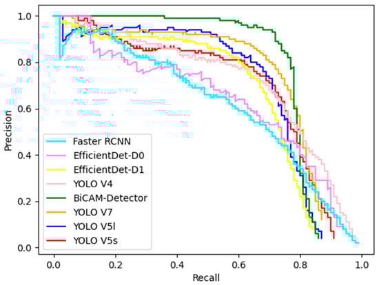
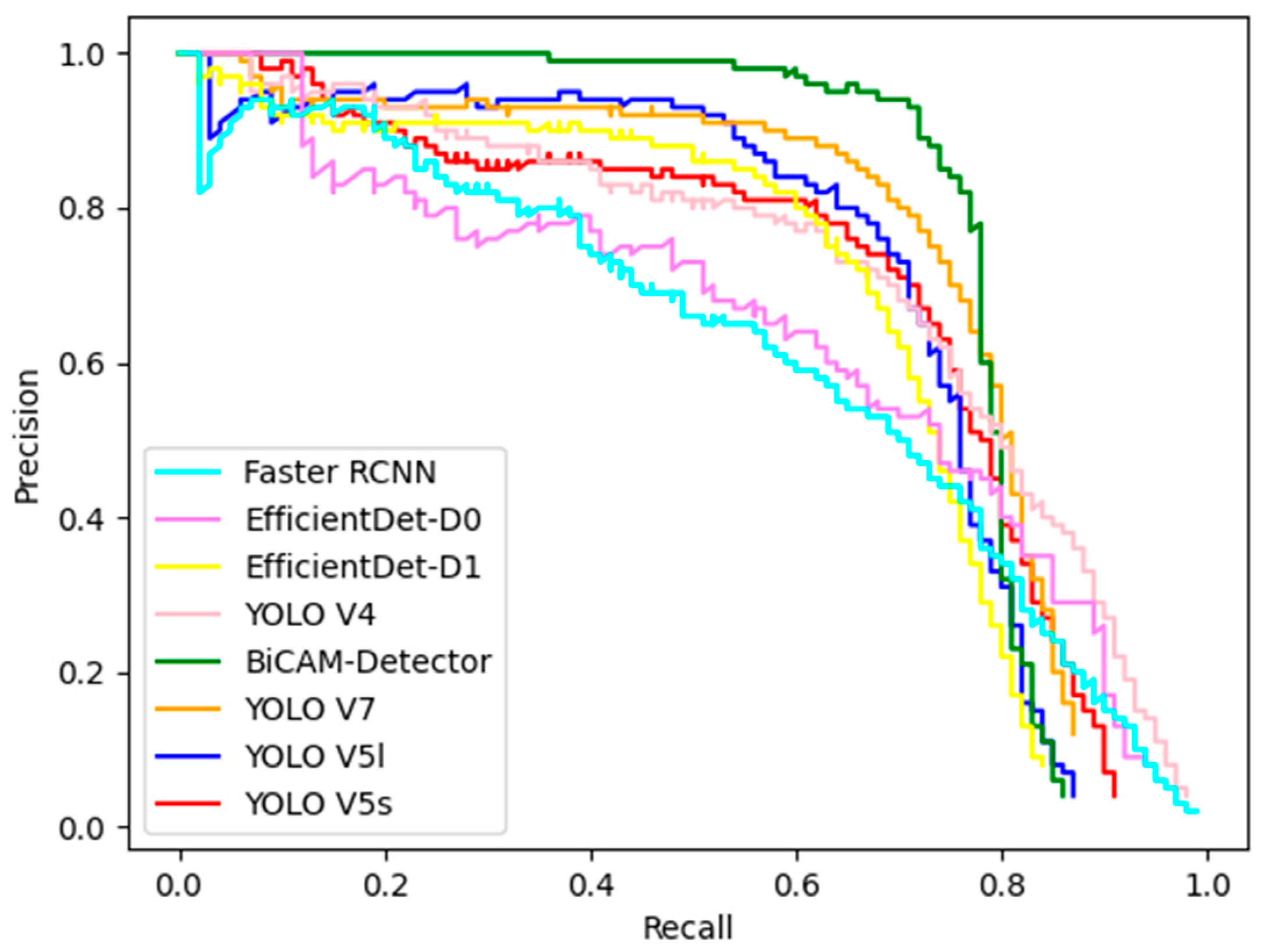
Figure 12.
The PR curves of BiCAM-Detector and the comparison algorithm on the DOTA1.5 dataset.
- (b)
- Experimental results on VEDAI
The VEDAI dataset contains a large number of weak and small objects, imposing high requirements on the detector. The comparative experimental results of our approach and other comparison models on this dataset are exhibited in Table 7 and Figure 13.
Table 7.
The experimental results on the VEDAI dataset.
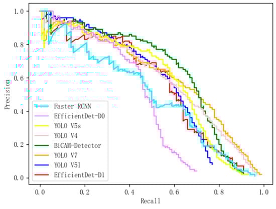
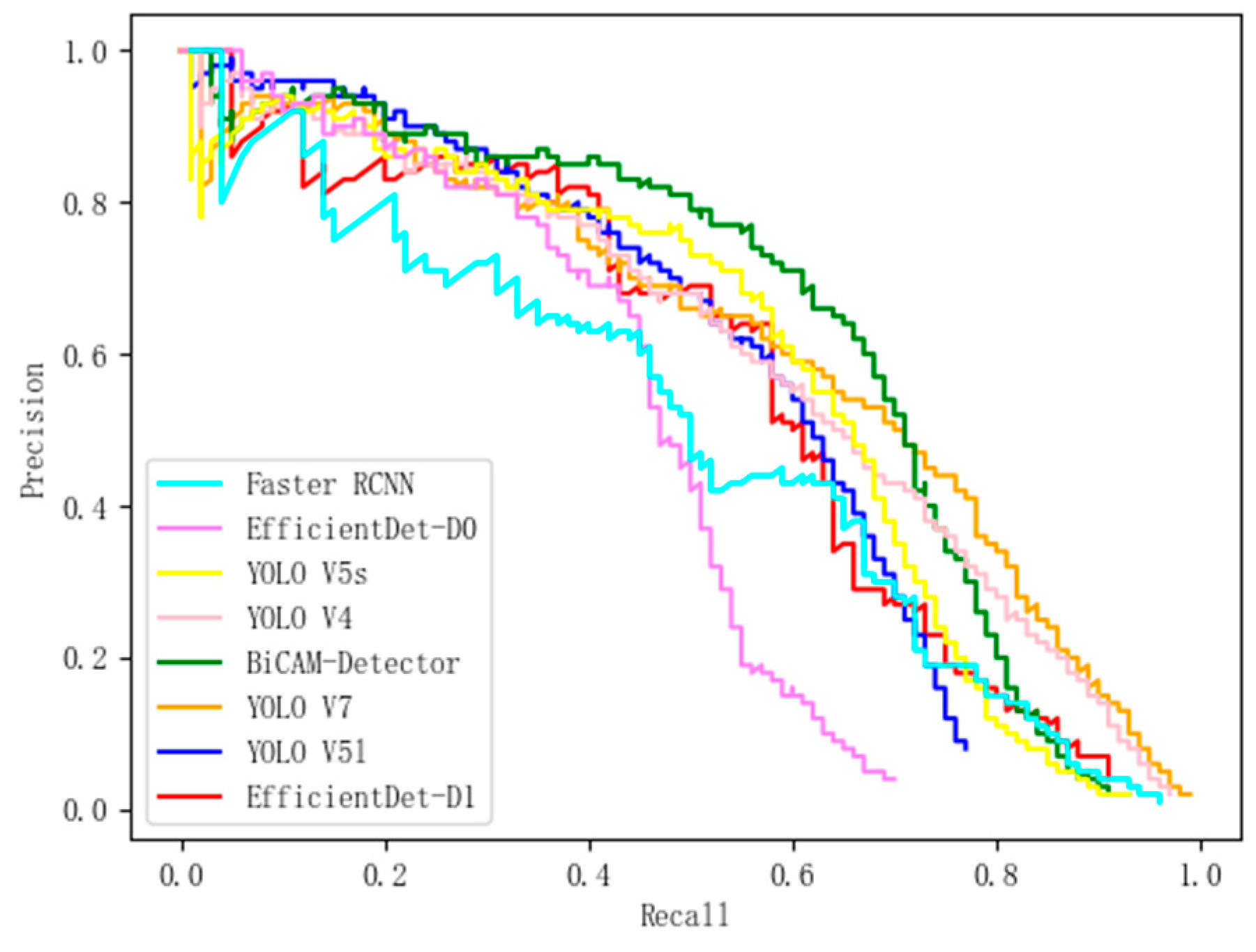
Figure 13.
The PR curves of BiCAM-Detector and comparison algorithm on the VEDAI dataset.
The experimental results shown in Table 6 and Table 7 have verified the superiority of our approach. The BiCAM-Detector achieves the optimal mean average precision with the comparison algorithms in both datasets. On the DOTA1.5 dataset, the mAP of our approach is 77.07%, and our approach achieves the highest accuracy in 12 out of 16 categories. Compared with advanced YOLO series algorithms such as YOLO V4, YOLO V5s, YOLO V5l and YOLO V7, the mAP of our approach is improved by 4.48%, 6.77%, 5.72%, and 2.51%, respectively. Compared with RTMDet, our approach can still achieve better performance. The mAP of our approach is improved by 1.06%. VEDAI dataset poses a greater challenge to the performance of detectors, as it contains a large number of objects with small sizes. The mAP of each detector is significantly reduced compared to the mAP on the DOTA1.5 dataset. The BiCAM-Detector proposed in this paper can still have good performance on VEDAI, with a mAP of 63.83%. The highest AP is obtained in 5 of the 8 categories. In addition, compared with YOLO V4, YOLO V5s, YOLO V5l, and YOLO V7, the mAP of our approach is improved by 4.23%, 7.96%, 6.28%, and 2.78% respectively. In contrast to the advanced SuperYOLO, the mAP of our approach is slightly improved by 0.75%. According to the PR curves in Figure 12 and Figure 13, our approach achieves best performance on DOTA1.5 and VEDAI, which proves the superiority of our approach.
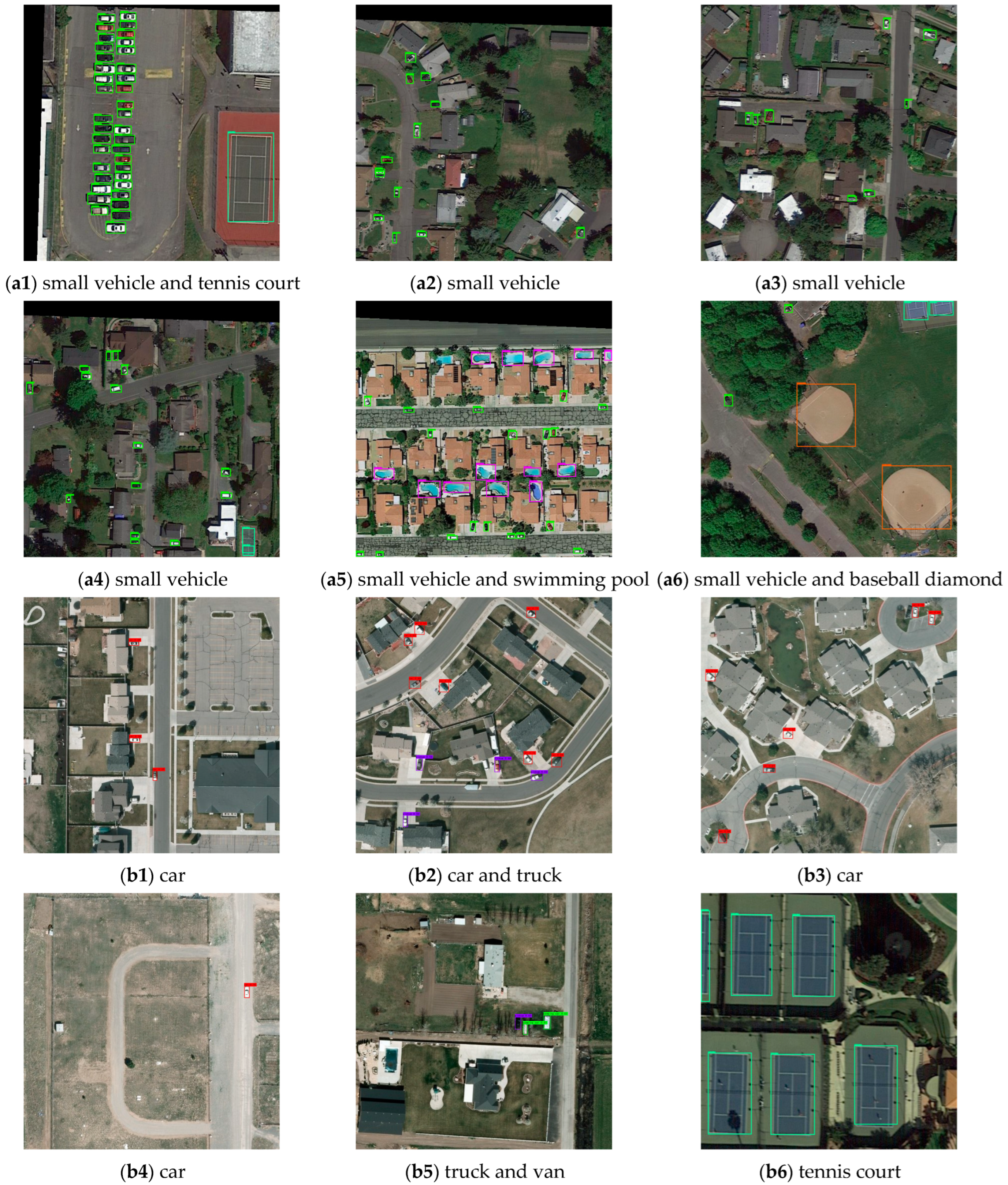
In Figure 14, we present the partial detection results of BiCAM-Detector on two datasets. The samples contain various types of scenes and many small objects. As can be seen from Figure 14, our approach can not only effectively detect densely distributed objects, small objects, and multi-shaped objects in remote sensing images, but also have good adaptability to complex environments.
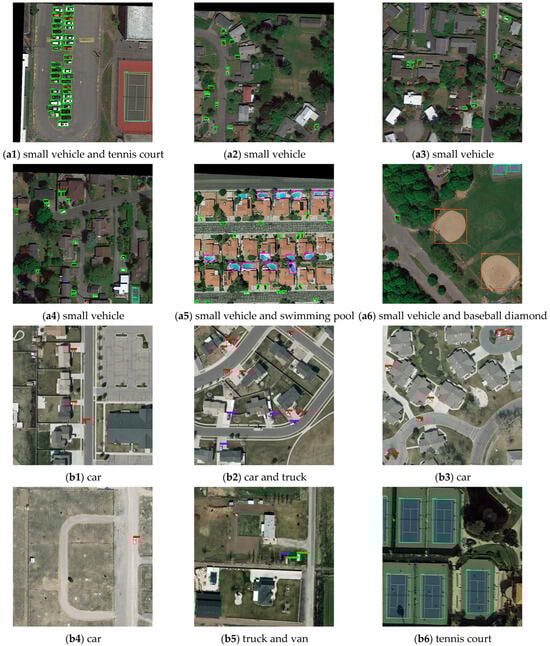
Figure 14.
The detection results of DOTA dataset. (a1–a6) The detection results on the DOTA1.5 dataset and (b1–b6) the detection results on the VEDAI dataset.
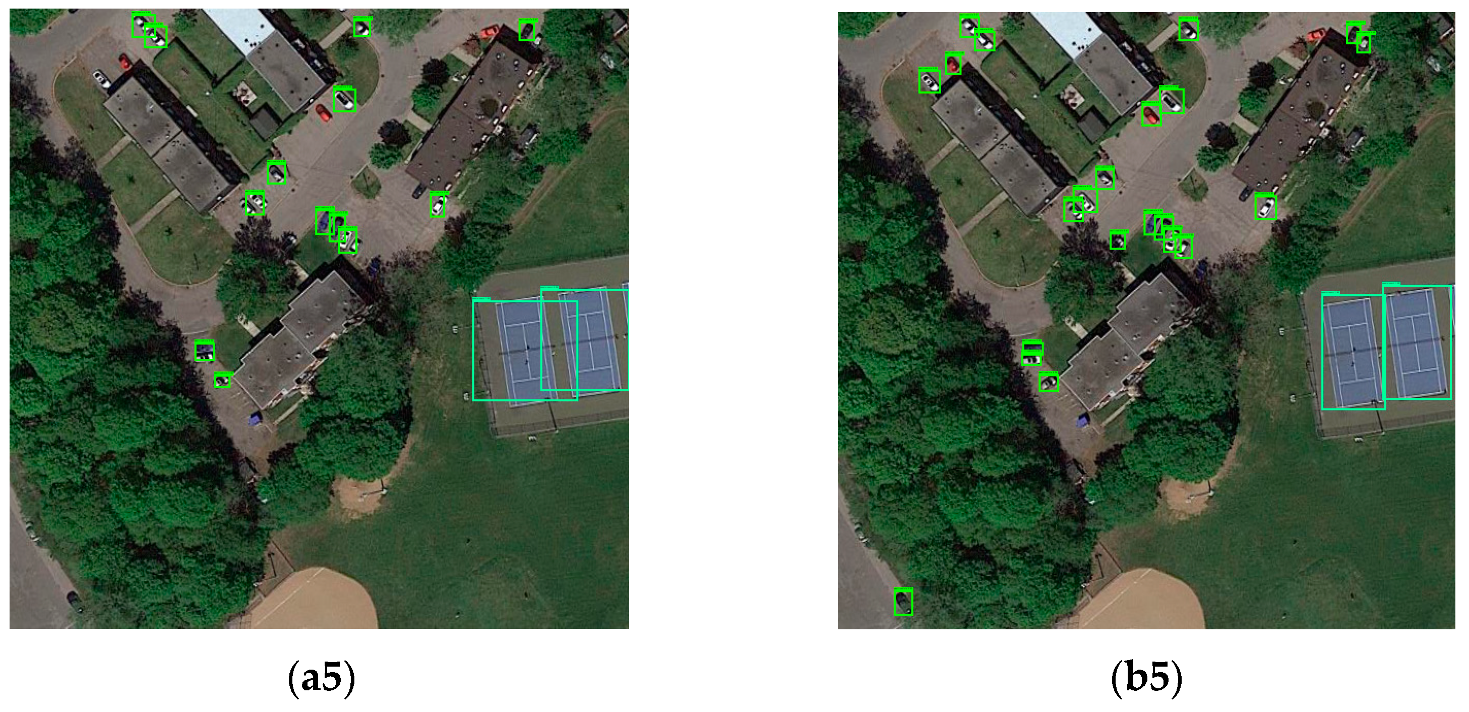
In addition, in order to highlight the superiority of our approach in small object detection in remote sensing images, we select YOLO V7 for comparison. The comparison results are shown in Figure 15.
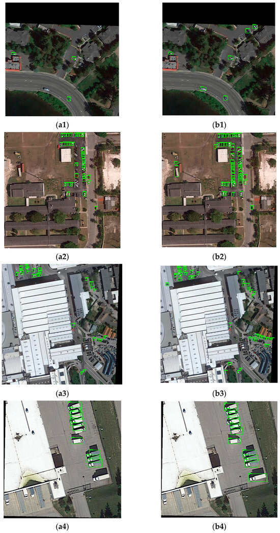
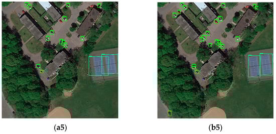
Figure 15.
Comparison of the partial detection results between BiCAM-Detector and YOLO V7. (a1–a5) The detection results of YOLO V7, and (b1–b5) the detection results of YOLO V7.
As shown in Figure 15, compared with YOLO V7, our approach has better performance, which further verifies the superiority of our approach in detecting small remote sensing objects.
In addition, Table 8 shows the comparison of real-time performance between our approach and other algorithms.
Table 8.
The real-time performance of each model.
Table 8 has verified that the BiCAM-Detector achieves the highest mAP under the conditions of the same input size and number of detection layers. The FPS of our approach is 42.9, which is higher than that of YOLO V4. Although the detection speed is lower than other comparison algorithms, the performance in mAP is superior.
4.4. Ablation Experiments
In order to verify the effectiveness of various improvement strategies proposed in this paper, we take DOTA1.5 as the experimental dataset and use different combinations of improvement strategies. The procedure for setting up the ablation experiments is as follows: We use the network with only backbone reduction as the Baseline and set it as Experiment 1. In Experiment 2, DC-CSP_n is added to the backbone network. In Experiment 3, CJAM-PRes2Net is adopted. In Experiment 4, CSP-CJAM-IRFE is used. In Experiment 5, Swin Transformer is added to the ‘Neck’ of the network. The anchor-free mechanism is adopted in Experiment 6. TIAN is added in Experiment 7.
The Baseline, which uses a streamlined backbone network, has the highest detection speed of 66.4 FPS, but its accuracy of 62.48% is lower. The use of CSP-CJAM-DPFE and CSP-Res2Net in the backbone network improves the mAP by 4.57% and 2.52%, respectively. The introduction of CSP-CJAM-IRFE improved the accuracy by 1.52%. The use of the Swin Transformer improved the accuracy by 2.38%. However, the detection speed will be greatly reduced from 55.3 FPS to 47.7 FPS. At the detection end, the anchor-free detection mechanism is adopted, which slightly improves the accuracy by 0.36%, and the FPS is increased from 47.7 to 52.4. In addition, Experiment 7 proves that the TIAN auxiliary network proposed in this paper can greatly improve the performance of the network, and the mAP is increased by 2.50%. In general, the experimental results in Table 9 have proved the effectiveness of each improvement.
Table 9.
The results of the ablation experiments on the DOTA1.5 dataset.
In order to verify the effectiveness of the CJAM, Table 10 compares the performance of CJAM with CBAM and E-ACAM.
Table 10.
The comparison of different attention mechanisms.
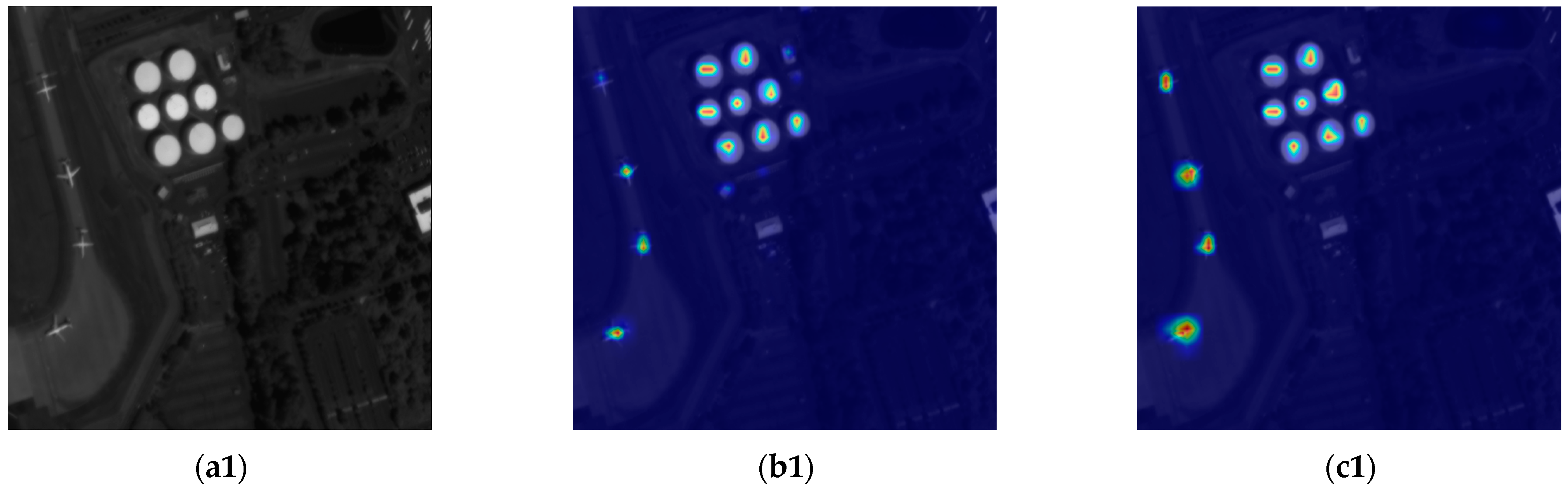
From Experiments 1 and 2 in Table 10 it can be seen that, compared with CBAM, CJAM proposed in this paper improves the mAP of the network by 2.38%. Compared with E-ACAM, CJAM improves the mAP of the network by 1.57%. From the perspective of detection speed, the detection speed of the network using CBAM is the lowest, with only 38.6 FPS. The CJAM proposed in this paper reaches the second-best detection speed, second only to E-ACAM, but the mAP is higher than it. Figure 16 shows the heatmaps of some samples.
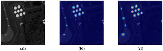
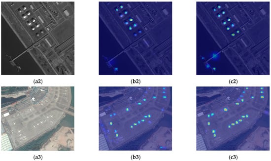
Figure 16.
The comparison of heatmaps between CBAM and CJAM. (a1–a3) The original image, (b1–b3) the heatmaps of CBAM, and (c1–c3) the heatmaps of CJAM.
In Figure 16, the heatmaps of CJAM can cover the area of a small object more perfectly than the heatmaps of CBAM. Combined with the test results in Table 10 and Figure 16, the superiority of CJAM is proved.
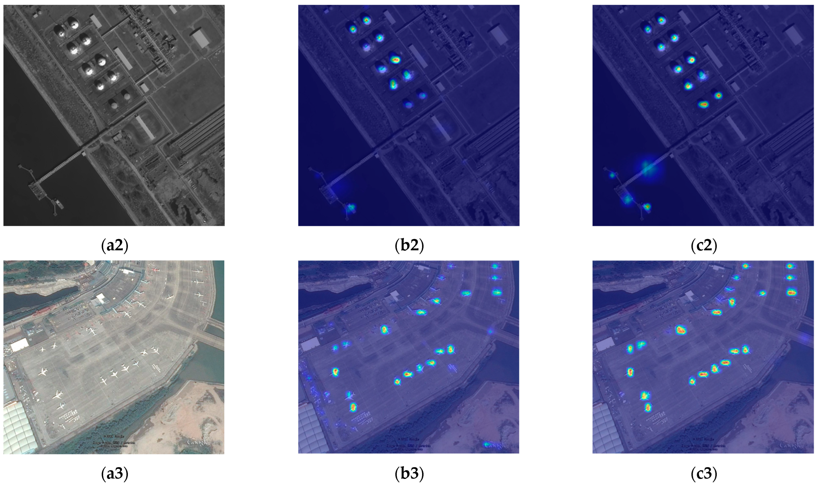
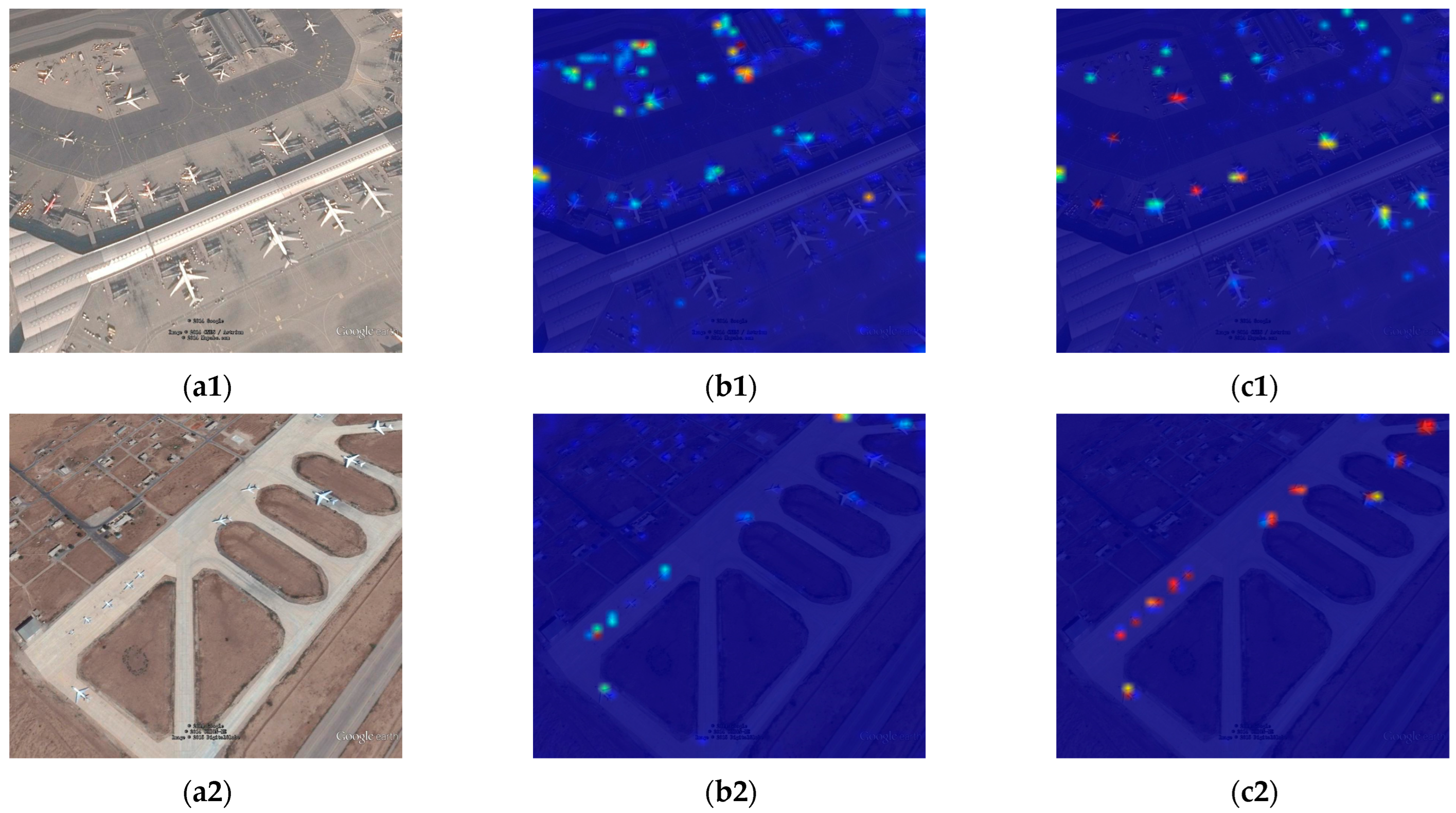
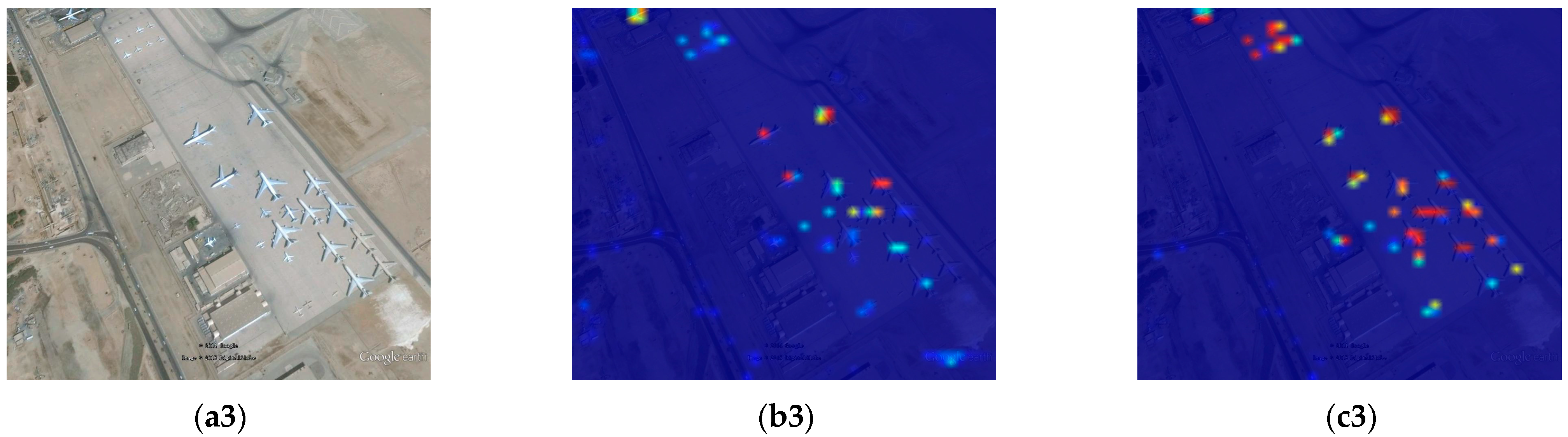
In order to test the performance of the auxiliary network TIAN, Figure 17 selects some samples and shows the Grad-CAM of their bottom layers. The bottom layer can pay more attention to the small objects.
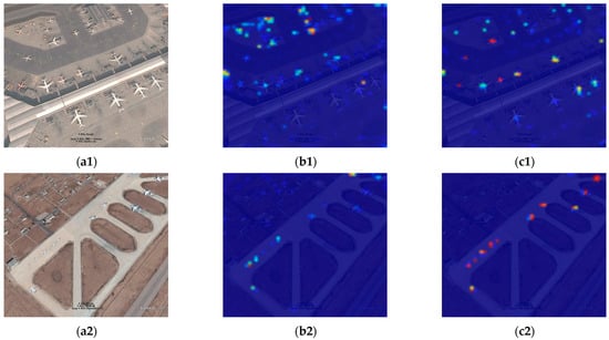
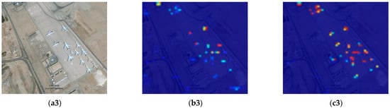
Figure 17.
The Grad-CAM images. (a1–a3) is the original image, (b1–b3) is the Grad-CAM images of the network without TIAN. (c1–c3) is the Grad-CAM images of the network with TIAN.
It can be seen in Figure 17, with TIAN added to the network that the detector can pay more attention to the small objects. The performance of the network to locate small objects is superior.
5. Discussion
The experimental results have verified the superior performance of BiCAM-Detector. The number of objects in the datasets we select is large, and the two datasets contain a large number of densely distributed and small-sized objects. The shapes of the objects is also diverse. The comparison experiments in Table 6 and Table 7 show that compared with other excellent algorithms, such as YOLO V4, YOLO V5s, YOLO V5l, and YOLO V7, the algorithm proposed in this paper has the highest mAP.
The comparison results show that the algorithm in this paper has better detection effect than YOLO V7 when facing small objects with dense distribution. In addition, for multi-directional objects, the algorithm in this chapter can also maintain a good detection effect.
In addition, ablation experiments have been carried out. The simplified backbone network can maintain a high detection speed, but the mAP is low. The analysis shows that the performance of the lightweight backbone network is limited. Although a series of improvement measures reduce the detection speed to a certain extent, mAP is greatly improved. The improved CJAM proposed in this paper gains the highest mAP and the detection speed is sub-optimal in the comparison attention mechanisms. The results of the heatmap comparison have also verified the excellent performance of CJAM on object feature extraction. Furthermore, the Grad-CAM images shows that the TIAN proposed in this paper can locate small objects effectively.
Based on the above discussion, our approach can maintain a good balance between accuracy and speed in detecting remote sensing objects. The performance of our approach is better than other advanced models.
6. Conclusions and Future Prospects
In the past few decades, CNN-based object detectors have made great progress. However, remote sensing object detection usually faces the problems of scale diversity, shape diversity, distribution density, and background complexity. The above problems bring difficulties in detecting remote sensing objects. In this paper, an efficient remote sensing object detector is proposed. A lightweight network is used for higher detection efficiency. The detection scales are adjusted to adapt to the detection of densely distributed objects. CJAM is proposed based on CBAM for better performance when facing a complex environment. DPFE and IRFE are adopted for feature enhancement and sensitivity to object scale diversity. In addition, TIAN and Swin transformer are added for object location and the improvement of the performance. The test results on DOTA1.5 and VEDAI datasets show that the proposed algorithm achieves 77.7% and 63.83%, respectively on mAP, which has better performance compared to other advanced detectors. Moreover, the detection speed of our approach is also satisfactory.
At present, remote sensing object detection still has a large room for development, and the future development directions are mainly as follows: (1) The backbone network is of great concern for feature extraction. Therefore, its structural breakthrough is the key, and the backbone network designed for the features of remote sensing image will be the focus of future research. (2) When dealing with very large datasets, accurately labeling objects is an extremely labor-intensive task. Therefore, high-precision weakly supervised detectors will be a promising development direction. (3) For the densely distributed objects, the horizontal bounding boxes will limit the performance of object detection. Therefore, the oriented bounding boxes are more suitable for the detection of densely distributed objects.
Author Contributions
Conceptualization, D.X. and Y.W.; Methodology, D.X.; Software, D.X.; Validation, D.X. and Y.W.; Formal analysis, D.X.; Investigation, D.X.; Resources, D.X.; Data curation, D.X.; Writing—original draft preparation, D.X. and Y.W.; Writing—review and editing, D.X.; Visualization, D.X.; Project administration, D.X.; Funding acquisition, D.X. All authors have read and agreed to the published version of the manuscript.
Funding
This research received no external funding.
Data Availability Statement
Not applicable.
Acknowledgments
The authors wish to thank the editor and reviewers for their suggestions and thank Yiquan Wu for his guidance.
Conflicts of Interest
The authors declare no conflict of interest.
References
- Zhou, D.X. Deep distributed convolutional neural networks: Universality. Anal. Appl. 2018, 16, 895–919. [Google Scholar] [CrossRef]
- Mirkhan, M.; Meybodi, M.R. Restricted Convolutional Neural Networks. Neural Process. Lett. 2019, 50, 1705–1733. [Google Scholar] [CrossRef]
- Gu, J.X.; Wang, Z.H.; Kuen, J.; Ma, L.Y.; Shahroudy, A.; Shuai, B.; Liu, T.; Wang, X.X.; Wang, G.; Cai, J.F.; et al. Recent advances in convolutional neural networks. Pattern Recognit. 2018, 77, 354–377. [Google Scholar] [CrossRef]
- Sarigul, M.; Ozyildirim, B.M.; Avci, M. Differential convolutional neural network. Neural Networks 2019, 116, 279–287. [Google Scholar] [CrossRef] [PubMed]
- Krichen, M.J.C. Convolutional neural networks: A survey. Computers 2023, 12, 151. [Google Scholar] [CrossRef]
- Alahmari, F.; Naim, A.; Alqahtani, H. E-Learning Modeling Technique and Convolution Neural Networks in Online Education. In IoT-enabled Convolutional Neural Networks: Techniques and Applications; River Publishers: Aalborg, Denmark, 2023; pp. 261–295. [Google Scholar]
- Girshick, R.; Donahue, J.; Darrell, T.; Malik, J. Rich feature hierarchies for accurate object detection and semantic segmentation. In Proceedings of the IEEE Conference on Computer Vision and Pattern Recognition, Columbus, OH, USA, 23–28 June 2014; pp. 580–587. [Google Scholar]
- Girshick, R. Fast r-cnn. In Proceedings of the IEEE International Conference on Computer Vision, Santiago, Chile, 7–13 December 2015; pp. 1440–1448. [Google Scholar]
- Ren, S.; He, K.; Girshick, R.; Sun, J. Faster r-cnn: Towards real-time object detection with region proposal networks. In Proceedings of the NIPS’15: Proceedings of the 28th International Conference on Neural Information Processing Systems, Montreal, QC, Canada, 7–12 December 2015. [Google Scholar]
- He, K.; Gkioxari, G.; Dollár, P.; Girshick, R. Mask r-cnn. In Proceedings of the IEEE International Conference on Computer Vision, Venice, Italy, 22–29 October 2017; pp. 2961–2969. [Google Scholar]
- Redmon, J.; Divvala, S.; Girshick, R.; Farhadi, A. You only look once: Unified, real-time object detection. In Proceedings of the IEEE Conference on Computer Vision and Pattern Recognition, Las Vegas, NV, USA, 27–30 June 2016; pp. 779–788. [Google Scholar]
- Redmon, J.; Farhadi, A. YOLO9000: Better, faster, stronger. In Proceedings of the IEEE Conference on Computer Vision and Pattern Recognition, Honolulu, HI, USA, 21–26 July 2017; pp. 7263–7271. [Google Scholar]
- Redmon, J.; Farhadi, A. Yolov3: An incremental improvement. arXiv 2018, arXiv:1804.02767. [Google Scholar]
- Bochkovskiy, A.; Wang, C.Y.; Liao, H.Y. Yolov4: Optimal speed and accuracy of object detection. arXiv 2020, arXiv:2004.10934. [Google Scholar]
- Wu, W.; Liu, H.; Li, L.; Long, Y.; Wang, X.; Wang, Z.; Li, J.; Chang, Y. Application of local fully Convolutional Neural Network combined with YOLO v5 algorithm in small target detection of remote sensing image. PLoS ONE 2021, 16, e0259283. [Google Scholar] [CrossRef]
- Li, C.; Li, L.; Jiang, H.; Weng, K.; Geng, Y.; Li, L.; Ke, Z.; Li, Q.; Cheng, M.; Nie, W.; et al. YOLOv6: A single-stage object detection framework for industrial applications. arXiv 2022, arXiv:2209.02976. [Google Scholar]
- Liu, W.; Anguelov, D.; Erhan, D.; Szegedy, C.; Reed, S.; Fu, C.-Y.; Berg, A.C. Ssd: Single shot multibox detector. In Proceedings of the Computer Vision–ECCV 2016: 14th European Conference, Amsterdam, The Netherlands, 11–14 October 2016; pp. 21–37. [Google Scholar]
- Fu, C.Y.; Liu, W.; Ranga, A.; Tyagi, A.; Berg, A.C. Dssd: Deconvolutional single shot detector. arXiv 2017, arXiv:1701.06659. [Google Scholar]
- Li, Z.; Zhou, F. FSSD: Feature fusion single shot multibox detector. arXiv 2017, arXiv:1712.00960. [Google Scholar]
- Li, J.; Li, Z.; Chen, M.; Wang, Y.; Luo, Q.J.R.S. A new ship detection algorithm in optical remote sensing images based on improved R3Det. Remote Sens. 2022, 14, 5048. [Google Scholar] [CrossRef]
- Zhang, H.; Liu, F.; Fan, Y.; Tan, F.; Qian, Y. FAFFENet: Frequency attention and feature fusion enhancement network for multiscale remote sensing target detection. J. Appl. Remote Sens. 2022, 16, 014512. [Google Scholar] [CrossRef]
- Teng, Z.; Duan, Y.; Liu, Y.; Zhang, B.; Fan, J.J.I.T.o.G.; Sensing, R. Global to local: Clip-LSTM-based object detection from remote sensing images. IEEE Trans. Geosci. Remote Sens. 2021, 60, 5603113. [Google Scholar] [CrossRef]
- Zhou, L.; Zheng, C.; Yan, H.; Zuo, X.; Liu, Y.; Qiao, B.; Yang, Y.J.I.I.J.o.G.-I. RepDarkNet: A Multi-Branched Detector for Small-Target Detection in Remote Sensing Images. ISPRS Int. J. Geo-Inf. 2022, 11, 158. [Google Scholar] [CrossRef]
- Hou, Y.; Shi, G.; Zhao, Y.; Wang, F.; Jiang, X.; Zhuang, R.; Mei, Y.; Ma, X.J.S. R-YOLO: A YOLO-Based Method for Arbitrary-Oriented Target Detection in High-Resolution Remote Sensing Images. Sensors 2022, 22, 5716. [Google Scholar] [CrossRef] [PubMed]
- Long, H.; Chung, Y.; Liu, Z.; Bu, S.J.I.A. Object detection in aerial images using feature fusion deep networks. IEEE Access 2019, 7, 30980–30990. [Google Scholar] [CrossRef]
- Yang, X.; Sun, H.; Fu, K.; Yang, J.; Sun, X.; Yan, M.; Guo, Z. Automatic ship detection in remote sensing images from google earth of complex scenes based on multiscale rotation dense feature pyramid networks. Remote Sens. 2018, 10, 132. [Google Scholar] [CrossRef]
- Azimi, S.M.; Vig, E.; Bahmanyar, R.; Körner, M.; Reinartz, P. Towards multi-class object detection in unconstrained remote sensing imagery. In Proceedings of the Asian Conference on Computer Vision, Perth, Australia, 2–6 December 2018; pp. 150–165. [Google Scholar]
- Wang, X.; Jiang, Y.; Luo, Z.; Liu, C.-L.; Choi, H.; Kim, S. Arbitrary shape scene text detection with adaptive text region representation. In Proceedings of the IEEE/CVF Conference on Computer Vision and Pattern Recognition, Long Beach, CA, USA, 15–20 June 2019; pp. 6449–6458. [Google Scholar]
- Xu, Z.; Xu, X.; Wang, L.; Yang, R.; Pu, F.J.R.S. Deformable convnet with aspect ratio constrained nms for object detection in remote sensing imagery. Remote Sens. 2017, 9, 1312. [Google Scholar] [CrossRef]
- Ren, Y.; Zhu, C.; Xiao, S.J.R.S. Deformable faster r-cnn with aggregating multi-layer features for partially occluded object detection in optical remote sensing images. Remote Sens. 2018, 10, 1470. [Google Scholar] [CrossRef]
- Wang, Y.; Jia, Y.; Gu, L.J.R.S. EFM-Net: Feature extraction and filtration with mask improvement network for object detection in remote sensing images. Remote Sens. 2021, 13, 4151. [Google Scholar] [CrossRef]
- Cheng, G.; Si, Y.; Hong, H.; Yao, X.; Guo, L.J.I.G.; Letters, R.S. Cross-scale feature fusion for object detection in optical remote sensing images. EEE Geosci. Remote Sens. Lett. 2020, 18, 431–435. [Google Scholar] [CrossRef]
- Niu, Z.; Zhong, G.; Yu, H.J.N. A review on the attention mechanism of deep learning. Neurocomputing 2021, 452, 48–62. [Google Scholar] [CrossRef]
- Soydaner, D.J.N.C. Applications. Attention mechanism in neural networks: Where it comes and where it goes. Neural Comput. Appl. 2022, 34, 13371–13385. [Google Scholar] [CrossRef]
- Zhu, H.; Xie, C.; Fei, Y.; Tao, H.J.E. Attention mechanisms in CNN-based single image super-resolution: A brief review and a new perspective. Electronics 2021, 10, 1187. [Google Scholar] [CrossRef]
- Ghaffarian, S.; Valente, J.; Van Der Voort, M.; Tekinerdogan, B.J.R.S. Effect of attention mechanism in deep learning-based remote sensing image processing: A systematic literature review. Remote Sens. 2021, 13, 2965. [Google Scholar] [CrossRef]
- Hu, J.; Shen, L.; Sun, G. Squeeze-and-excitation networks. In Proceedings of the IEEE Conference on Computer Vision and Pattern Recognition, Salt Lake City, UT, USA, 18–22 June 2018; pp. 7132–7141. [Google Scholar]
- Wang, Q.; Wu, B.; Zhu, P.; Li, P.; Zuo, W.; Hu, Q. ECA-Net: Efficient channel attention for deep convolutional neural networks. In Proceedings of the IEEE/CVF Conference on Computer Vision and Pattern Recognition, Seattle, WA, USA, 14–19 June 2020; pp. 11534–11542. [Google Scholar]
- Woo, S.; Park, J.; Lee, J.-Y.; Kweon, I.S. Cbam: Convolutional block attention module. In Proceedings of the European Conference on Computer Vision (ECCV), Munich, Germany, 8–14 September 2018; pp. 3–19. [Google Scholar]
- Chen, Y.; Li, J.; Xiao, H.; Jin, X.; Yan, S.; Feng, J. Dual path networks. In Proceedings of the 31st Conference on Neural Information Processing Systems (NIPS 2017), Long Beach, CA, USA, 4–9 December 2017. [Google Scholar]
- Szegedy, C.; Liu, W.; Jia, Y.; Sermanet, P.; Reed, S.; Anguelov, D.; Erhan, D.; Vanhoucke, V.; Rabinovich, A. Going deeper with convolutions. In Proceedings of the IEEE Conference on Computer Vision and Pattern Recognition, Boston, MA, USA, 7–12 June 2015; pp. 1–9. [Google Scholar]
- Ioffe, S.; Szegedy, C. Batch normalization: Accelerating deep network training by reducing internal covariate shift. In Proceedings of the International Conference on Machine Learning, Lille, France, 6–11 July 2015; pp. 448–456. [Google Scholar]
- Szegedy, C.; Vanhoucke, V.; Ioffe, S.; Shlens, J.; Wojna, Z. Rethinking the inception architecture for computer vision. In Proceedings of the IEEE Conference on Computer Vision and Pattern Recognition, Las Vegas, NV, USA, 27–30 June 2016; pp. 2818–2826. [Google Scholar]
- He, K.; Zhang, X.; Ren, S.; Sun, J. Spatial pyramid pooling in deep convolutional networks for visual recognition. IEEE Trans. Pattern Anal. Mach. Intell. 2015, 37, 1904–1916. [Google Scholar] [CrossRef]
- Vaswani, A.; Shazeer, N.; Parmar, N.; Uszkoreit, J.; Jones, L.; Gomez, A.N.; Kaiser, Ł.; Polosukhin, I. Attention is all you need. In Proceedings of the 31st Conference on Neural Information Processing Systems (NIPS 2017), Long Beach, CA, USA, 4–9 December 2017. [Google Scholar]
- Liu, Z.; Lin, Y.; Cao, Y.; Hu, H.; Wei, Y.; Zhang, Z.; Lin, S.; Guo, B. Swin transformer: Hierarchical vision transformer using shifted windows. In Proceedings of the IEEE/CVF International Conference on Computer Vision, Virtual, 11–17 October 2021; pp. 10012–10022. [Google Scholar]
- Tian, Z.; Shen, C.; Chen, H.; He, T. Fcos: Fully convolutional one-stage object detection. In Proceedings of the IEEE/CVF International Conference on Computer Vision, Seoul, Republic of Korea, 27 October–2 November 2019; pp. 9627–9636. [Google Scholar]
- Xia, G.-S.; Bai, X.; Ding, J.; Zhu, Z.; Belongie, S.; Luo, J.; Datcu, M.; Pelillo, M.; Zhang, L. DOTA: A large-scale dataset for object detection in aerial images. In Proceedings of the IEEE Conference on Computer Vision and Pattern Recognition, Salt Lake City, UT, USA, 18–22 June 2018; pp. 3974–3983. [Google Scholar]
- Razakarivony, S.; Jurie, F. Vehicle detection in aerial imagery (vedai): A benchmark. J. Vis. Commun. Image Represent. 2015, 34, 187–203. [Google Scholar] [CrossRef]
- Lyu, C.; Zhang, W.; Huang, H.; Zhou, Y.; Wang, Y.; Liu, Y.; Zhang, S.; Chen, K. Rtmdet: An empirical study of designing real-time object detectors. arXiv 2022, arXiv:2212.07784. [Google Scholar]
- Zhang, J.; Lei, J.; Xie, W.; Fang, Z.; Li, Y.; Du, Q. SuperYOLO: Super resolution assisted object detection in multimodal remote sensing imagery. IEEE Trans. Geosci. Remote Sens. 2023, 61, 5605415. [Google Scholar] [CrossRef]

Disclaimer/Publisher’s Note: The statements, opinions and data contained in all publications are solely those of the individual author(s) and contributor(s) and not of MDPI and/or the editor(s). MDPI and/or the editor(s) disclaim responsibility for any injury to people or property resulting from any ideas, methods, instructions or products referred to in the content. |
© 2023 by the authors. Licensee MDPI, Basel, Switzerland. This article is an open access article distributed under the terms and conditions of the Creative Commons Attribution (CC BY) license (https://creativecommons.org/licenses/by/4.0/).