Abstract
In order to deal with the problem space-time adaptive processing (STAP) performance degradation of an airborne phased array system caused by the serious shortage of independent and identical distributed (IID) training samples in the nonhomogeneous clutter environment, an improved direct data domain method based on sparse Bayesian learning is proposed in this paper, which only uses a single snapshot data of a cell under test (CUT) to suppress the clutter and has fast computational speed. Firstly, three hyper-parameters required to obtain the sparse solution are derived. Secondly, the comparative analysis of their iterative formulas is made, and the piecewise iteration of hyper-parameter that has an obvious influence on the computational complexity of obtaining sparse solution is presented. Lastly, with the approximate prior information of the target, the clutter sparse solution is given and its covariance matrix is effectively estimated to calculate the adaptive filter weight and realize the clutter suppression. Simulation results verify that the proposal can dramatically decrease the computational burden while keeping the superior heterogeneous clutter suppression performance.
1. Introduction
Strong ground clutter needs to be effectively suppressed when an airborne radar detects a low-altitude moving target. Due to the motion of the aircraft platform, the Doppler bandwidth of clutter is rapidly broadened and the clutter spatial-temporal coupling property is generated. As a result, the target is often submerged in the strong background clutter. To this problem, typical space-time adaptive processing (STAP) [1] is introduced, which estimates the clutter covariance matrix (CCM) of cells under test (CUT) mainly by using a lot of independent and identical distributed (IID) training samples to realize the clutter suppression [2,3]. However, in an actual clutter environment, the remarkable heterogeneity is one of the important characteristics of clutter because some external factors exist such as the variation of topography, strong scattering point, and electromagnetic interference. Furthermore, the number of IID samples decreases and it is hard to satisfy the requirement. This phenomenon may be aggravated with the complications of the electromagnetic environment. At last, the clutter suppression performance of STAP is worsened.
In recent years, for the sake of solving this problem, many improved methods have been put forward such as reduced-rank STAP, reduced-dimension STAP, parametric STAP, knowledge-aided STAP, and direct data domain STAP [4,5,6,7,8,9]. Even though the required IID samples available are reduced, the existing IID sample size used to achieve the favorable CCM estimation is not still enough, or they are at the cost of sacrificing system processing capacity. Especially with the inhomogeneity of ground clutter further aggravated, the IID sample size is rapidly shortened and the performance of mainly current clutter suppression methods will be severely deteriorated. In addition, the new system radar is concerned, for example, about the multiple-input multiple-output (MIMO) system [10,11]. Combined with MIMO and STAP techniques, though the virtual synthetic aperture is achieved by transmitting waveform diversity, the heavy computational burden is also difficult to realize the effective response.
At the same time, sparse recovery (SR) technique appears, which is widely applied to many fields, for example, radar imaging [12] and clutter suppression [13,14]. On the basis of this approach, Bayesian learning algorithms are particularly concerned, and sparse Bayesian learning (SBL) is one of the important sparse solution methods that have been generally utilized to realize the reconstruction of sparse signals [15,16]. They can use a few training samples, even only one sample to accomplish CCM estimation, which greatly reduce the requirement for IID training samples; however, due to sparse discretization, the large computational load is also increased. For this case, many improved SR algorithms are researched, for example, reduced-dimension sparse recovery (RD-SR) [17,18] and temporal SBL [19,20]. Even though the computational burden can be effectively decreased, the dependence of them for training samples is still difficult to eliminate.
Based on the above analysis, a comprehensive consideration of the computational complexity and extreme shortage of training samples in severely nonhomogeneous clutter environment, a fast heterogeneous clutter suppression method with improved direct data domain (DDD) based on sparse Bayesian learning (SBL) is proposed in this paper. The proposal has many advantages in severely heterogeneous clutter suppression. Firstly, only a single frame of CUT data needs to be used for realizing the nonhomogeneous clutter suppression, which solves the problem that many current methods rely heavily on training samples. At the same time, the influence of the quality of training samples and the number of IID samples on STAP performance can be completely eliminated by the approach. Secondly, the rough prior knowledge of target under test is effectively utilized to realize the elimination of target components in the proposal, which can avoid its influence on CCM estimation. Meanwhile, the sacrifice of system degrees of freedom caused by the DDD method can also be overcome. Thirdly, the influence of SBL hyper-parameter iterations on the computational complexity will be analyzed in this paper. By the piecewise processing of the proposed method, the phenomenon of high dimension and slow iteration in the initial iteration stage is avoided. Meanwhile, the speed is moderately slowed down in the later iteration stage to maintain and ensure the sparse recovery accuracy. Therefore, this method has the superior ability of relieving the contradiction between computation and performance. The main processing of the approach can be divided into three stages.
- Obtaining the single CUT data. Since only CUT is directly analyzed and utilized in the proposed method, the initial step is to realize the sparse representation of data to be used in the subsequent handling of SR-STAP.
- Calculating the sparse solution. In view of the space-time relevance of the inner structure on clutter data, a fast SBL method attempts to be applied to sparse solution calculation. This stage can also be regarded as the iteration of hyper-parameters. In order to alleviate the conflict between computational complexity and sparse solution accuracy, three hyper-parameters are compared and analyzed. By finding the main hyper-parameter affecting the calculating burden, a kind of piecewise processing is put forward in the approach. Overall, different iteration formulas are reasonably utilized in the initial stage with a higher parameter dimension and the late stage with a lower parameter dimension.
- Estimating CCM based on rough prior knowledge. With the aid of approximate prior information of CUT, the target component is removed and CCM is estimated.
The remaining content of this paper is arranged as follows: the signal model with SR-STAP is given in Section 2; the improved DDD method based on SBL is particularly described and analyzed in Section 3; some simulation experiments are shown to verify the effectiveness of the proposal in Section 4; and the relevant conclusions are drawn in Section 5.
2. Signal Model with SR-STAP
Suppose the airborne side-looking uniform linear array (ULA) has receiving elements, is the receiving element interval and is the radar wavelength. and represent the pulse repetition interval (PRI) and the number of pulses in a coherent processing interval (CPI), respectively. The flight velocity and height of airborne plane are and . The echo data of CUT can be denoted as
where is the number of clutter patches, and are separately the clutter scattering intensity and interested target scattering intensity, and represent the clutter and target spatial-temporal steering vectors, , are the normalized temporal frequencies of clutter and target, , are the normalized spatial frequencies of clutter and target, is the noise signal.
Considering the sparsity of echo data in space-time plane, Equation (1) can be further expressed as
where and are respectively, the number of quantified discrete grid points in temporal domain and spatial domain, , are separately the sparse dictionary and sparse solution, which can be defined as
where , are the spatial-temporal steering vector and sparse value of grid point , , represent the normalized Doppler frequency and spatial frequency of grid point , , .
3. Improved DDD Method Based on SBL
In view of the spatial-temporal correlation of clutter inner structure, sparse Bayesian learning framework [21,22,23,24] can be applied to calculate the sparse solution of CUT.
Since belongs to the complex domain and Bayesian criterion is mainly applicable to real domain, Equation (2) should be further transformed as
where , are the operations of obtaining the real part and the imaginary part.
By Equation (4), the dimensions of , , , are , , , and . If () submits to Gauss distribution and its mean is zero, the likelihood function of Equation (4) can be defined as
where is the variance of (), is the identity matrix.
Meanwhile, suppose that () is independent and obeys Gauss distribution, its probability distribution satisfies
where and are non-negative hyper-parameters. reflects the signal sparsity, and presents time correlation within sparse solution. The relative position of sparse solution has no significant value when equals to zero [25].
Then, according to Equation (6), the prior distribution of sparse vector can be denoted as
where , is the diagonal matrix, is the Hadamard product.
Furthermore, needs to be replaced by a same hyper-parameter for eliminating the overfitting phenomenon, and .
Hence, Equation (7) is also described as
where is the Kronecker product.
Combined with Equations (5)–(8), the posteriori Gauss distribution of is expressed as [26]
where and are separately presented as , .
Furthermore, the maximum posteriori estimation of sparse solution about CUT is defined as
Combined with Equations (9) and (10), it can be seen that calculating and is transformed into obtaining the iterative formulas of these hyper-parameters , , . Namely, these hyper-parameters need to be gradually iterated in the acquisition process of sparse solution . To this point, a kind of cost function is introduced as [27]
By solving the minimization of cost function in Equation (11), the suitable hyper-parameter values are effectively acquired. In reference [19], the expectation-maximization method [28,29] is applied to estimating the hyper-parameters , , . The iterative formulas of three hyper-parameters can be described, respectively, as
where , is the diagonal element of .
Moreover, in reference [30], for the sake of promoting the operating speed of sparse Bayesian, the fixed-point (FP) method [31] is adopted to obtain the hyper-parameter . The iterative formulas of three hyper-parameters can be denoted, respectively, as
Compared with Equation (12), it can be seen that the iteration of hyper-parameters and are similar in Equation (13). However, the iteration of is obviously changed. Therefore, the iterative process of is the main reason of affecting the computational complexity of sparse solution estimation.
Based on the above analysis, a new iteration of hyper-parameter is given to reduce the computational burden in this paper. It can be expressed as
Then, combined with Equations (12) and (13), the faster method of calculating hyper-parameters is proposed, which can be denoted as
where , is the number of element that satisfies , is the threshold of pruning the small hyper-parameter .
The ultimate purpose of piecewise calculation in Equation (15) is that the total iterative speed of hyper-parameter is further quickened while guaranteeing the accuracy of . Considering that is bigger in the initial phase of iteration, the latter iteration formula needs to be selected so that can be rapidly declined and the iterative time is shortened. However, when is smaller in the late stage, the former iteration formula needs to be chosen so as to be gradually reduction inthe iterative speed and ensure the precision of . Hence, based on Equation (15), the proposed iterative algorithm can not only reduce the computational complexity in the initial stage, but also keep accuracy in the late stage. It is beneficial to obtain the sparse solution in the heterogeneous clutter environment.
With the help of the iterative formulas of , , in Equation (15), the mean vector and covariance matrix in Equation (9) are obtained. Then, by using Equation (10), the sparse solution can be estimated. In view of the fact that the target component is contained in the sparse solution, the rough prior information of target under test can be used to remove the target component and estimate CCM. Suppose that the spatial prior area and temporal prior area are separately , , CCM is expressed as
where is the clutter sparse solution, which is equal to zero when and , and are the scope factors of approximate temporal and spatial prior information about the target under test, is the noise power, is the imaginary unit.
According to Equation (16), the adaptive weight can be estimated to realize the heterogeneous clutter suppression.
Based on processing steps of the proposed method, the theoretical analysis is provided. From part two, it can be seen that the dimension of CUT data , sparse dictionary , and sparse solution are , , and , respectively. Considering the actual application of SBL, these three vectors are transformed into , , and . Their dimensions are , , and , separately. When SBL is used to obtain the sparse solution , the iteration of hyper parameters is crucial. The hyper parameter reflects the signal sparsity, which denotes the arbitrary element of . The hyper parameter presents time correlation within sparse solution. The hyper parameter is the variance of noise. In terms of these three hyper parameters, only parameter () needs to be iteratively calculated on the whole discrete points. Its solving process plays a decisive role in computational burden of SBL. Therefore, the iterative calculation of is one of the important factors affecting the computational efficiency of SBL algorithms. For the above reasons, the original number of sparse discrete points is , which is applied to dividing point of the hyper parameter segmentation processing. When is in the initial iteration stage, the calculation is more about parameter initialization. This stage has little effect on the sparse recovery performance of the algorithm, but has great influence on the computational complexity of the algorithm. Meanwhile, the dimension of large parameter values is generally higher in the initial iteration stage. Thus, the second iterative formula of Equation (14) is adopted when the dimension of is bigger than , which can rapidly decrease the dimension of and avoid the phenomenon of slow iteration. However, when the dimension of is smaller than , the first iterative formula of Equation (14) is utilized, which can ensure the sparse recovery accuracy. As a result, the contradiction between computation and performance of SBL can be effectively relieved by this segmented iteration scheme.
4. Simulation Analyses
In this section, some simulation experiments are made to demonstrate the heterogeneous clutter suppression performance of the proposed method. Relevant parameters are set as follows: the number of receiving elements and pulses are 16, 8; radar wavelength is 0.23, pulse repetition frequency is 2434.8 Hz, receiving element interval is 0.115; velocities of airborne plane and target are 140 m/s and 28 m/s, flight height is 8000 m; the number of trials is 30; signal-to-noise ratio and clutter-to-noise ratio are separately 20 dB and 60 dB; and the normalized temporal frequency and spatial frequency of interested target are 0.4, 0. Moreover, four sparse recovery methods such as SBL [32,33], temporally sparse Bayesian learning (TSBL) [19,34], temporally sparse Bayesian learning with FP method (TSBL-FP) [35], the improved TSBL method (IMP-TSBL) [36] and the proposed method in this paper are applied and compared. The results are shown in Figure 1, Figure 2 and Figure 3.
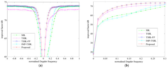
Figure 1.
Improved factor (IF) against normalized Doppler frequency: (a) Local comparison in the vertical direction, (b) Local comparison in the horizontal direction.
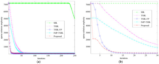
Figure 2.
Computational complexity of different methods in the sparse solution calculation: (a) Comparison with 250 iterations, (b) Comparison with 30 iterations.
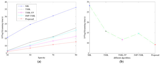
Figure 3.
Running time comparison of five different methods in the sparse solution calculation: (a) Comparison with different sparsity, (b) Comparison when sparsity is 60.
In Figure 1, from the perspective of improved factor (IF), the nonhomogeneous clutter suppression performance with five different methods is compared and analyzed. The IF is usually adopted as one of important indicators to measure STAP performance, which is equal to the ratio of output signal-to-clutter-plus-noise ratio to input signal-to-clutter-plus-noise ratio. Moreover, when the IF gap near the normalized Doppler frequency 0 becomes narrower and deeper, it indicates STAP method can better suppress the clutter. If the gap gets widened and shallower, it denotes that the method has worse nonhomogeneous clutter suppression performance and more residual clutter is contained at the output of STAP. Thus, among five different methods, local comparison with the vertical direction (60–75 dB) is made to present the width of the IF gap in Figure 1a, and local comparison with the horizontal direction (0–0.3) is made to present the depth of the IF gap in Figure 1b. According to these two results, it can be seen that the proposed method has a similar clutter suppression performance with TSBL-FP. Meanwhile, their performances on STAP are better than IMP-TSBL, SBL and TSBL under the same condition of only using single snapshot CUT data. As for IMP-TSBL, least square estimation and threshold setting of average energy superposition function are mainly applied to reduction in algorithm iterations so as to decline the computational complexity. It can also be regarded as a kind of reduced-dimension SBL method. Though the column dimension of sparse dictionary is forced down, it leads to the loss of partial useful information before the hyper-parameter iteration. As a result, the performance of this method is decreased.
In Figure 2, the computational complexity of five different methods is given, which is used to verify the STAP efficiency. Since obtaining the sparse solution process is the main step of improving the SR-STAP speed, the sparse solution complexity with each iteration is displayed, and the total calculation burden is equal to the sum of them. In descending order, these methods are arranged one by one such as SBL, TSBL, IMP-TSBL, TSBL-FP, and the proposed method. Even if TSBL-FP has the similar clutter suppression performance with the proposed method, the computational load of the latter is significantly less than that of the former, especially in the initial stage of algorithm iteration. Moreover, the sparse solution complexity of the initial iteration is critical, which can directly affect the iterative trend of algorithm. Therefore, the piecewise iteration formula is applied in the proposed method for settling the problem of large iterative computation in the initial period and keeping the effectiveness of sparse recovery. Based on the result with 250 iterations in Figure 2a, the convergence of acquiring the sparse solution is obviously shown. Furthermore, the convergence speed of the initial iteration is emphatically presented in Figure 2b. As for the proposal, it can be seen that the sparse solution complexity is sharply decreased between the first and the second iteration. Meanwhile, before the ninth iteration, the complexity of the proposed method is evidently smaller than that of TSBL-FP. In terms of IMP-TSBL, the column dimension of the sparse dictionary is obviously decreased before hyper-parameter iteration. Correspondingly, the number of participating in the iteration is also dropped rapidly when the parameter starts the first iteration. As a result, the computational burden of IMP-TSBL is smaller than SBL and TSBL. Whereas, since the iterative speed of this method slows down, the overall computational complexity of this method is bigger than the approach in this paper.
In Figure 3, the running time of SBL method in the sparse solution calculation is adopted to visually analyze its computational complexity. Comparison with different sparsity is denoted in Figure 3a. Comparison with a same sparsity is given in Figure 3b when sparsity is 60. If sparsity of SBL is 60, it means that and are both 60. Correspondingly, is equal to 3600. From Figure 3a, it can be seen that the running time of all methods will become longer with the increasing of sparsity. In descending order of running time under the same sparsity, these methods are generally arranged one by one such as SBL, TSBL, IMP-TSBL, TSBL-FP, and the proposal. When sparsity is 30, the last four methods have a similar running time. The reason is that since the number of grid points on a sparse dictionary is smaller, the performance difference of these four methods is not obvious. Overall, the approach is still better than the others; however, as the sparsity increases, the difference in running time between the proposed method and other methods is gradually widened. It is attributed to the benefit of piecewise iteration. From Figure 3b, it can be seen that when sparsity is equal to 60, the difference in computational speed of sparse solution is evidently amplified, which is matched with the whole variation in Figure 3a.
5. Conclusions
In this paper, based on sparse Bayesian learning framework, a novel heterogeneous clutter suppression method using improved direct data domain is proposed and verified, which has the ability to promote the timelessness of STAP in the nonhomogeneous clutter environment. The proposal can effectively suppress the clutter only using one snapshot data of the cell under test regardless of the heterogeneity of training samples. By analysis and piecewise iteration of the hyper-parameter that has influence on calculating sparse solution, the computational complexity of STAP is dramatically declined and the proposed method still has superior clutter suppression performance. Some simulations demonstrate the effectiveness of the proposal. Overall, significant contributions of the approach are mainly divided into four points. Firstly, aiming at the problem of STAP clutter suppression in severely nonhomogeneous clutter environment, a novel knowledge-aided scheme is provided in this paper. It can improve STAP processing performance in case of extreme shortage of IID training samples. Secondly, the computational complexity is significantly declined using this proposal, which further promotes the practicability of SBL and STAP in actual conditions. Thirdly, the iteration of hyper-parameters is one of the important factors affecting the computational efficiency of SBL algorithms, which is reasonably analyzed and utilized in this paper. Moreover, the proposal can provide a new idea for the research and promotion of SBL algorithms. Fourthly, a different perspective for low-altitude target detection of an airborne radar in a complex electromagnetic environment is given by the proposed method, which has certain application prospects in the fields of early warning detection and low-altitude area surveillance.
Author Contributions
Q.W. and Z.L. proposed the signal model and clutter suppression method; Q.W., Y.Z. and W.Z. constructed and designed the simulation experiments; Z.L. and Y.Z. completed the paper writing; W.Z. and Q.W. put the finishing touches to this paper. All authors have read and agreed to the published version of the manuscript.
Funding
This research was funded by the National Natural Science Foundation of China under Grant 62001479(Wang, Q.), by the School Scientific Research Program of National University of Defense Technology under Grants ZK19-28(Wang, Q.).
Conflicts of Interest
The authors declare no conflict of interest.
References
- Brennan, L.E.; Reed, L.S. Theory of adaptive radar. IEEE Trans. Aerosp. Electron. Syst. 1973, 9, 237–252. [Google Scholar] [CrossRef]
- Wu, D.; Zhu, D.Y.; Shen, M.W.; Li, N.; Zhou, H.Y. Clutter suppression for wideband radar STAP. IEEE Trans. Geosci. Remote Sens. 2022, 60, 1–18. [Google Scholar] [CrossRef]
- Li, X.Z.; Xie, W.C.; Wang, Y.L. A training sample selection method based on united generalized inner product statistics for STAP. IET Radar Sonar Navig. 2021, 15, 1565–1572. [Google Scholar] [CrossRef]
- Yang, Z.C.; Wang, X.Y. Reduced-rank space-time adaptive processing algorithm based on multistage selection of angle-Doppler filters. IET Radar Sonar Navig. 2022, 16, 327–345. [Google Scholar] [CrossRef]
- Huang, P.H.; Zou, Z.H.; Xia, X.G.; Liu, X.Z.; Liao, G.S. A novel dimension-reduced space-time adaptive processing algorithm for space-borne multichannel surveillance radar systems based on spatial-temporal 2-D sliding window. IEEE Trans. Geosci. Remote Sens. 2022, 60, 1–21. [Google Scholar]
- Zhao, K.; Liu, Z.W.; Shi, S.L.; Huang, Y.L.; Xu, Y.G. Augmented joint domain localized method for polarimetric space-time adaptive processing. Circ. Syst. Signal Process. 2021, 40, 3592–3608. [Google Scholar] [CrossRef]
- Klintberg, J.; Mckelvey, T.; Dammert, P. A parametric approach to space-time adaptive processing in bistatic radar systems. IEEE Trans. Aerosp. Electron. Syst. 2022, 58, 1149–1160. [Google Scholar] [CrossRef]
- Chen, H.M.; Liu, J.; Sun, H.W.; Yi, X.L.; Mu, H.Q.; Lu, Y.B. Knowledge-aided space time adaptive processing for airborne radar in heterogeneous environments. In Proceedings of the 2019 IEEE International Conference on Signal, Information and Data Processing (ICSIDP), Chongqing, China, 11–13 December 2019; pp. 1–5. [Google Scholar]
- Gao, Z.Q.; Tao, H.H. Knowledge-aided direct data domain STAP algorithm for forward-looking airborne radar. In Proceedings of the 2019 IEEE International Conference on Signal, Information and Data Processing (ICSIDP), Chongqing, China, 11–13 December 2019; pp. 1–6. [Google Scholar]
- Wen, F.Q.; Gui, G.; Gacanin, H.; Sari, H. Compressive sampling framework for 2D-DOA and polarization estimation in mmwave polarized massive MIMO systems. IEEE Trans. Wirel. Commun. 2022. [Google Scholar] [CrossRef]
- Wen, F.Q.; Shi, J.P.; Gui, G.; Gacanin, H.; Dobre, O.A. 3-D positioning method for anonymous UAV based on bistatic polarized MIMO radar. IEEE Internet Things J. 2023, 10, 815–827. [Google Scholar] [CrossRef]
- Xu, G.; Zhang, B.J.; Yu, H.W.; Chen, J.L.; Xing, M.D.; Hong, W. Sparse synthetic aperture radar imaging form compressed sensing and machine learning: Theories, applications, and trends. IEEE Geosci. Remote Sens. M. 2022, 2–40. [Google Scholar] [CrossRef]
- Cui, N.; Xing, K.; Yu, Z.J.; Duan, K.Q. Tensor-based sparse recovery space-time adaptive processing for large size data clutter suppression in airborne radar. IEEE Trans. Aerosp. Electron. Syst. 2022, 1–17. [Google Scholar] [CrossRef]
- Xia, D.P.; Zhang, L.; Wu, T.; Meng, X.D. A clutter suppression method for airborne bistatic polarization radar based on polarization space-time adaptive processing. Multidim. Syst. Signal Process. 2022, 33, 899–916. [Google Scholar] [CrossRef]
- Tipping, M.E. Sparse Bayesian learning and the relevance vector machine. J. Mach. Learn. Res. 2001, 1, 211–244. [Google Scholar]
- Wipf, D.P.; Rao, B.D. Sparse Bayesian learning for basis selection. IEEE Trans. Signal Process. 2004, 52, 2153–2164. [Google Scholar] [CrossRef]
- Zhang, W.; An, R.X.; He, N.Y.; He, Z.S.; Li, H.Y. Reduced dimension STAP based on sparse recovery in heterogeneous clutter environments. IEEE Trans. Aerosp. Electron. Syst. 2020, 56, 785–795. [Google Scholar] [CrossRef]
- Cui, W.C.; Wang, T.; Wang, D.G.; Liu, K. An efficient sparse Bayesian learning STAP algorithm with adaptive Laplace prior. Remote Sens. 2022, 14, 3520. [Google Scholar] [CrossRef]
- Zhang, Z.L.; Rao, B.D. Sparse signal recovery with temporally correlated source vectors using sparse Bayesian learning. IEEE J. Sel. Top. Signal Process. 2011, 5, 912–926. [Google Scholar] [CrossRef]
- Qiao, G.; Song, Q.J.; Ma, L.; Sun, Z.X.; Zhang, J.R. Channel prediction based temporal multiple sparse Bayesian learning for channel estimation in fast time-varying underwater acoustic OFDM communications. Signal Process. 2020, 175, 107668. [Google Scholar] [CrossRef]
- Cui, N.; Xing, K.; Duan, K.Q.; Yu, Z.J. Fast tensor-based three-dimensional sparse Bayesian learning space-time adaptive processing method. J. Radar 2021, 10, 919–928. [Google Scholar]
- Wang, G.S.; Wang, Y.Q.; Huang, G.C.; Ren, Q.H.; Ren, T.T. Simultaneous sparse learning algorithm of structured approximation with transformation analysis embedded in Bayesian framework. J. Electron. Imaging 2021, 30, 053006. [Google Scholar] [CrossRef]
- Xu, X.W.; Zhang, S.; Gao, F.F.; Wang, J.Z. Sparse Bayesian learning based channel extrapolation for RIS assisted MIMO-OFDM. IEEE Trans. Commun. 2022, 70, 5498–5513. [Google Scholar] [CrossRef]
- Li, H.R.; Dai, J.S.; Pan, T.H.; Chang, C.Q.; So, H.C. Sparse Bayesian learning approach for baseline correction. Chemometr. Intell. Lab. Syst. 2020, 204, 104088. [Google Scholar] [CrossRef]
- Zhang, Z.L.; Rao, B.D. Extension of SBL algorithms for the recovery of block sparse signals with intra-block correlation. IEEE Trans. Signal Process. 2013, 61, 2009–2015. [Google Scholar] [CrossRef]
- Wang, Q.S.; Yu, H.; Li, J.; Ji, F.; Chen, F.J. Sparse Bayesian learning using generalized double pareto prior for DOA estimation. IEEE Signal Process. Lett. 2021, 28, 1744–1748. [Google Scholar] [CrossRef]
- Cui, N.; Xing, K.; Duan, K.Q.; Yu, Z.J. Knowledge-aided block sparse Bayesian learning STAP for phased-array MIMO airborne radar. IET Radar Sonar Navig. 2021, 15, 1628–1642. [Google Scholar] [CrossRef]
- Moon, T.K. The expectation-maximization algorithm. IEEE Signal Process. Mag. 1996, 13, 47–60. [Google Scholar] [CrossRef]
- Zhou, W.; Zhang, H.T.; Wang, J. Sparse Bayesian learning based on collaborative neurodynamic optimization. IEEE Trans. Cybernetics 2022, 52, 13669–13683. [Google Scholar] [CrossRef]
- Wang, B.; Zhu, Z.; Dai, Y. A fast underwater acoustic target direction of arrival estimation method based on sparse Bayesian learning. Acta Acust. 2016, 41, 81–86. [Google Scholar]
- MacKay, D.J.C. Bayesian interpolation. Neural Comput. 1992, 4, 131–134. [Google Scholar] [CrossRef]
- Song, Q.J. Research on Sparse Bayesian Learning Based Sparse Channel Estimation in Underwater Acoustic OFDM Communication. Ph.D. Thesis, Harbin Engineering University, Harbin, China, November 2020. [Google Scholar]
- Liu, S.; Tang, L.; Bai, Y.C.; Zhang, X.G. A sparse Bayesian learning-based DOA estimation method with the Kalman filter in MIMO radar. Electronics 2020, 9, 347. [Google Scholar] [CrossRef]
- Cao, Z.; Dai, J.S.; Xu, W.C.; Chang, C.Q. Fast variational Bayesian inference for temporally correlated sparse signal recovery. IEEE Signal Process. Lett. 2021, 28, 214–218. [Google Scholar] [CrossRef]
- Wang, B.; Zhu, Z.H.; Dai, Y.W. On fast estimation of direction of arrival for underwater acoustic target based on sparse Bayesian learning. Chin. J. Acoust. 2017, 36, 102–112. [Google Scholar]
- Hong, D.Y.; Wang, W.; Yin, L.; Pu, Z.Q.; Zhou, C.Y.; Huang, H.N. An improved temporal multiple sparse Bayesian learning under-ice acoustic channel estimation method. Acta Acust. 2022, 47, 591–602. [Google Scholar]
Disclaimer/Publisher’s Note: The statements, opinions and data contained in all publications are solely those of the individual author(s) and contributor(s) and not of MDPI and/or the editor(s). MDPI and/or the editor(s) disclaim responsibility for any injury to people or property resulting from any ideas, methods, instructions or products referred to in the content. |
© 2023 by the authors. Licensee MDPI, Basel, Switzerland. This article is an open access article distributed under the terms and conditions of the Creative Commons Attribution (CC BY) license (https://creativecommons.org/licenses/by/4.0/).