Adaptive Line Enhancer Based on Maximum Correntropy Criterion and Frequency Domain Sparsity for Passive Sonars

Abstract

The low-frequency narrowband components (known as lines) in the radiated noise of underwater acoustic targets are an important feature of passive sonar detection. Conventional adaptive line enhancer (ALE) based on the least mean square algorithm has limited performance under colored background noise and low signal-to-noise ratio (SNR). In this paper, by combining the frequency domain sparse model of lines and maximum correntropy criterion (MCC), a β-adaptive l₀-MCC-ALE is proposed to solve the above-mentioned problem. The proposed ALE uses a sparse-driven MCC algorithm to update the weight vector in the frequency domain to further suppress the colored background noise. For the problem that the value of parameter β is sensitive to the performance, β is updated adaptively according to the frequency response of ALE in each iteration. Simulation and real data processing results show that the proposed ALE is insensitive to the given parameter β and has excellent performance for line enhancement. Compared with conventional ALE, the SNR of lines can be improved by 7~8 dB.

1. Introduction

Passive sonar systems have been widely used in underwater unmanned platforms to detect, locate, and identify targets by receiving and processing underwater acoustic signals. [1]. Radiated noise is the main object of passive sonar detection, which is composed of a wideband continuous spectrum and some narrowband discrete components [2]. The continuous spectrum is mainly caused by propeller cavitation. Narrowband components are usually generated by the ship’s mechanical vibration and propeller operation, which are known as lines [3]. With the continuous improvement of target concealment, the spectral level of the continuous spectrum of underwater acoustic targets is greatly reduced, and conventional energy detection methods make it difficult to detect the target effectively. However, low-frequency lines in radiated noise have the characteristics of long propagation distance and high signal-to-noise ratio (SNR) and represent the important feature of the target [4]. Therefore, line detection can improve the operating range of passive sonars, which is of great significance for underwater low-noise target detection [5].

Because of the complex marine environment, weak lines are often overwhelmed by strong noise and difficult to extract. In general, spatial processing gain and time processing gain are the two SNR gains sought by passive sonars. Spatial gain is generally obtained by array signal reception using a beamforming method [6]. However, due to the size of the underwater unmanned platform, the number and spacing of the array elements are limited, which makes it difficult to obtain the expected effect. Time gain is generally obtained by increasing the discrete Fourier transform (DFT) integration time, but it is not applicable to the case of non-stationary or the frequency shift of lines [7]. In the absence of any prior information, an adaptive line enhancer (ALE) is used as a preprocessing method for radiated noise to improve the SNR of lines in a certain integration time [8]. ALE is a special form of adaptive filter making use of the uncorrelation of wideband noise to improve the SNR through an adaptive algorithm, which has been widely used in speech, biomedicine, underwater acoustics, and other fields [9,10,11]. To date, passive sonar systems mainly use conventional ALE based on the least mean square (LMS) algorithm [12]. The LMS algorithm uses the squared error as the cost function, which is simple to implement and has low computational complexity. However, the weight vector obtained by the LMS algorithm will fluctuate around the steady-state solution, resulting in high steady-state misalignment, which limits the performance of the adaptive filter. Especially under low SNR, the performance of conventional ALE decreases rapidly and has limited improvement on the SNR of lines [13]. For passive sonar systems, ALE with stronger noise suppression ability needs to be studied.

From the perspective of the frequency domain, lines show sparsity in the frequency spectrum. To make full use of the frequency domain sparsity of lines, Hao et al. migrated adaptive algorithms of sparse systems to the frequency domain [14]. Three kinds of ALE, ZA, RZA, and l₀, were proposed according to different approximate methods of the l₀ norm and significantly improved the SNR of lines. Jin et al. generalized sparse constraints to the l_p norm and proposed an l_1/2-ALE to greatly improve the SNR of lines [15]. However, these algorithms are still based on LMS, and under the assumption of wideband white background noise, only the second-order statistics of the error signal are used. Considering that ocean ambient noise is generally colored, the above existing methods based on frequency domain sparsity lack targeted optimization. Its advantage is no longer under colored background noise, and the improvement is limited compared to the conventional ALE. Therefore, an ALE that can perform well under colored background noise is needed for passive sonars.

Recently, adaptive algorithms based on the maximum correntropy criterion (MCC) have been widely used in the application of adaptive filters, such as system identification, noise cancellation, channel estimation, etc. In these works, the conventional LMS algorithm is replaced by MCC, which further enhances the noise suppression ability to improve the performance of the adaptive filter [16,17,18]. Correntropy is a local similarity measure that includes all even moments and is robust to outliers [19]. The results show that MCC is not only effective in the non-Gaussian environment but also has a good suppression ability to colored background noise [20,21]. Qi et al. applied the Kalman filter based on MCC to TOA localization, which effectively suppressed the Gaussian-colored noise generated by multipath and nonlinear in the system [20]. Ahmad et al. proposed an estimator based on correntropy to achieve efficient parameter estimation under colored and non-Gaussian noise [21]. In order to make ALE have better performance under colored background noise, MCC is applied to the ALE of passive sonars in this paper.

By combining MCC with the frequency domain sparsity, a new l₀-MCC-ALE is proposed. It is iteratively updated in the frequency domain using l₀-pseudo-norm penalty and correntropy, which takes advantage of both sparse constraint and MCC. Further, a β-adaptive l₀-MCC-ALE with adaptive adjustment of parameter β is proposed to the problem that the performance of l₀-MCC-ALE is sensitive to parameter β. β-adaptive l₀-MCC-ALE can reduce the sensitivity of parameter β effectively, while ensuring the performance, reducing the cost of parameter β selection. Simulation and sea trail data analysis show that the proposed ALE has better performance for line enhancement under colored background noise, and the SNR of lines can be improved by 7~8 dB compared with conventional ALE.

The rest of this paper is organized as follows. In Section 2, convectional ALE, MCC, and frequency domain sparsity are introduced. In Section 3, β-adaptive l₀-MCC-ALE is proposed. Section 4 and Section 5 are simulation performance analysis and the results of real data processing, respectively. Finally, the work is summarized in Section 6.

2. Basic Theory

In this section, the signal model of conventional ALE and LMS algorithms are first introduced, which are the basis for our improvements. Secondly, the principles and steps of MCC are introduced. Finally, the frequency domain sparsity of lines is explained, which provides support for the proposed method.

2.1. Conventional ALE

The received radiated noise signal is composed of lines (single frequency components) and wideband noise. Assuming that the received time domain signal is x(n) and the wideband noise is v(n), the received signal can be expressed as:

$$x(n)=\sum _{m=0}^{M-1}{A}_m\sin \left(2\pi f_{m}n/f_s+{\phi }_m\right)+v(n),$$

(1)

where M is the number of lines, A_m, f_m and φ_m are the amplitude, frequency, and phase of the mth line, respectively, and f_s is the sampling rate.

Signal x(n) can be passed through an ALE to pre-enhance the lines. The structure of conventional ALE is shown in Figure 1. By making a delay of Δ points, the correlation of wideband noise no longer exists, while the correlation of lines is retained. Therefore, the irrelevant noise will be suppressed after passing through the filter. The output y(n) of ALE is the signal after the wideband noise is suppressed, which can be expressed as:

$$y(n)=w^{\mathrm{T}}(n)x(n-\Delta ),$$

(2)

where w(n) = [w₀(n), w₁(n), …, w_L−1(n)]^T is the weight vector, x(n − Δ) = [x(n − Δ), x(n − Δ − 1), …, x(n − Δ − L+1)]^T is the delayed input vector, L is the order of the adaptive filter and [∙]^T represents the transpose operation. Then the estimated error can be expressed as:

$$e(n)=x(n)-y(n).$$

(3)

The LMS algorithm uses the square of the error as the cost function, and updates the weight vector based on the steepest descent method:

$$w(n+1)=w(n)-\mu \frac{\partial J_{\mathrm{LMS}}(n)}{\partial w(n)}=w(n)+\mu e(n)x(n-\Delta ),$$

(4)

where μ is the step size. The performance of LMS is limited under low SNR for its high steady-state misalignment. Moreover, LMS is not suitable for colored background noise because it is based on the assumption of white noise and uses only second-order statistics of the error.

2.2. MCC

MCC uses correntropy to improve the adaptive algorithm. Correntropy is a nonlinear similarity measure. Specifically, given two random variables X and Y, with a finite number of N samples, the correntropy can be estimated as:

$$\widehat{V}(X,Y)=\frac{1}{N}\sum _{i=0}^{N-1}\kappa \left(x_i,y_i\right),$$

(5)

where κ(∙) represents a shift-invariant Mercer kernel, and the most commonly used is Gaussian kernel function:

$$\kappa (x,y)=\frac{1}{\sigma \sqrt{2\pi }}\exp \left(-\frac{e^2}{2{\sigma }^2}\right),$$

(6)

where e = x − y, σ is the standard deviation of the Gaussian distribution, called kernel width. Compared with other similarity measures, such as the mean square error (MSE), correntropy (with Gaussian kernel) has the following ideal properties [19]: (1) it is always bounded for any distribution; (2) all even moments are included, and the weight of higher moments is determined by the size of the kernel; (3) it is a local similarity measure, which is robust to outliers.

MCC uses correntropy as a measure of error, replaces the minimized square error by maximizing the correntropy estimated at the current iteration round n, and its cost function can be written as:

$$J_{\mathrm{MCC}}(n)=-\frac{1}{\sqrt{2\pi }\sigma }\exp \left(-\frac{e^2(n)}{2{\sigma }^2}\right).$$

(7)

Similarly, the updated formula of the weight vector can be obtained by using gradient descent as follows:

$$w(n+1)=w(n)-\mu \frac{\partial J_{\mathrm{MCC}}(n)}{\partial w(n)}=w(n)+\mu \exp \left(-\frac{e^2(n)}{2{\sigma }^2}\right)e(n)x(n-\Delta ).$$

(8)

MCC is not only simple to implement but also robust to different types of noise because of the properties of correntropy. At present, MCC is widely used in adaptive filters to suppress non-Gaussian noise and colored noise in systems. In this paper, it is applied to the ALE of passive sonars to suppress ocean ambient noise.

2.3. Frequency Domain Sparse Model

Lines are considered discrete narrowband components, which show ideal sparsity in the frequency spectrum. When a signal is enhanced by ALE, it passes through an FIR filter, and the ALE weight vector is the coefficient of the filter. The function of ALE is to enhance the energy at line frequency points and suppress the noise at other frequency points. Therefore, the ideal frequency response of the filter should be sparse, which is the frequency domain sparse model of ALE.

Consider a simple case where ALE input is assumed to consist of a line superimposed with noise, expressed as:

$$x(n)=A_0\sin (2\pi f_{0}n/f_s+{\phi }_0)+v(n).$$

(9)

According to [22], the optimal impulse response of an ideal ALE is also a sinusoidal sequence:

$$w_i^{opt}=a\cos (2\pi f_0(i+\Delta )/f_s),\hspace{1em}\hspace{1em}\hspace{1em}i=0,1,\dots ,L-1,$$

(10)

where

$$a=\frac{2(A_0^2/{\sigma }_v^2)}{2+L\cdot (A_0^2/{\sigma }_v^2)}.$$

(11)

The frequency response of the ideal ALE is the DFT of Equation (10):

$$W^{opt}(f)=\frac{a}{2}{e}^{\mathrm{j}2\pi f_0\Delta /f_s}{e}^{\mathrm{j}\pi (f_0-f)(L-1)/f_s}\frac{\sin (\pi (f_0-f)L/f_s)}{\sin (\pi (f_0-f)/f_s)}.$$

(12)

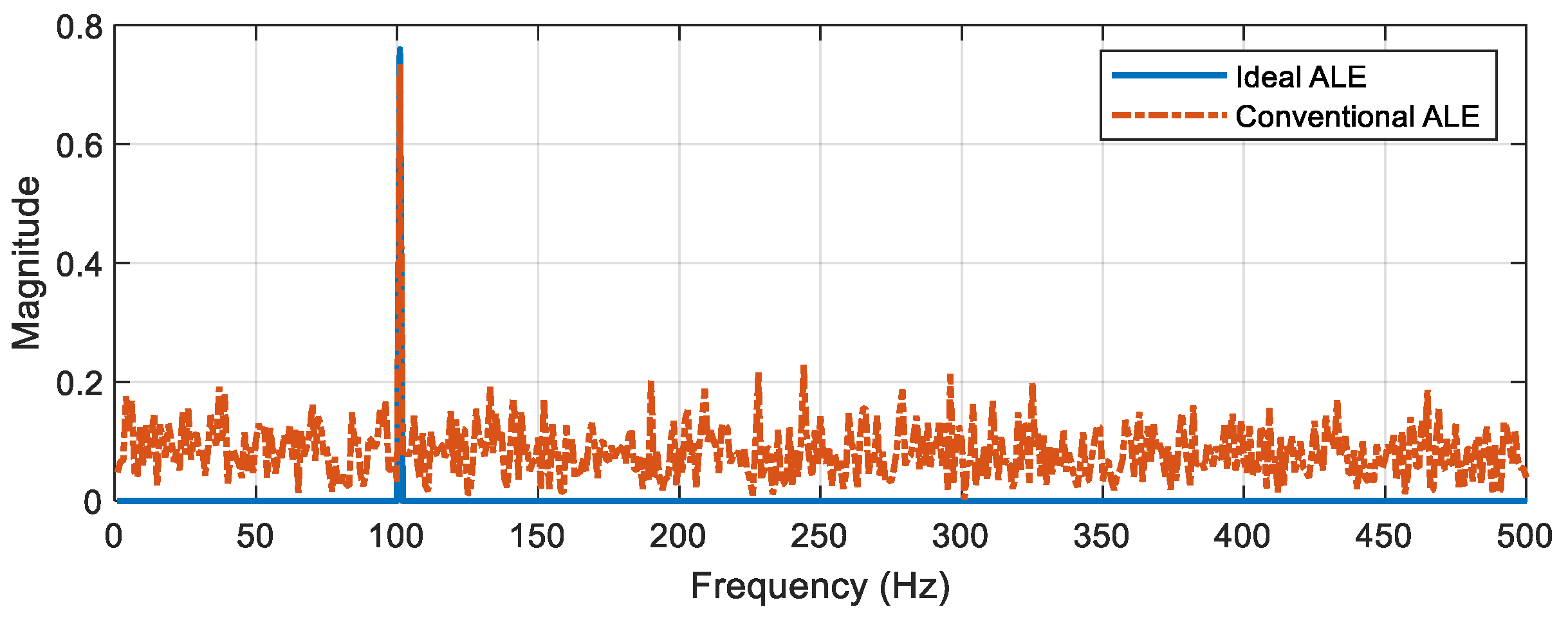
As can be seen from Equation (12), the magnitude of an ideal ALE only has a value of aL/2 at the line frequency point f₀, and is affected by the input SNR and the order, while other points are equal to zero. Therefore, the frequency response is sparse.

In practical applications, it is hoped that the frequency response of ALE can further approximate the ideal situation. Figure 2 shows the comparison of frequency response between the ideal ALE and the conventional ALE, in which the simulated line frequency is 100 Hz. Although the conventional ALE has been able to suppress noise, it is still far from the ideal sparse model and can be optimized. Therefore, the SNR of lines can be further improved by making the ALE frequency response sparser.

3. The Proposed Method

In this paper, we combine MCC with a frequency domain sparse model to deduce the l₀-MCC-ALE and β-adaptive l₀-MCC-ALE. The proposed method updates the weight vector in the frequency domain and uses the kernel function of MCC plus the l₀-pseudo-norm penalty as the cost function to improve the performance.

3.1. l₀-MCC-ALE

The frequency domain form of the ALE input vector can be expressed as:

$$x_F(n-\Delta )=Fx(n-\Delta ),$$

(13)

where F is the normalized DFT matrix:

$$F=\frac{1}{\sqrt{L}}\left[\begin{array}{ccccc}1& 1& 1& \cdots & 1\\ 1& e^{-\mathrm{j}(2\pi /L)}& e^{-\mathrm{j}(4\pi /L)}& \cdots & e^{-\mathrm{j}(2\pi (L-1)/L)}\\ ⋮& ⋮& ⋮& \ddots & ⋮\\ 1& e^{-\mathrm{j}(2\pi (L-1)/L)}& e^{-\mathrm{j}(4\pi (L-1)/L)}& \cdots & e^{-\mathrm{j}(2\pi {(L-1)}^2/L)}\end{array}\right].$$

(14)

Then, the ALE output y(n) can be expressed as:

$$y(n)=w^{\mathrm{T}}(n)F^{\mathrm{H}}Fx(k-\Delta )=w_F^{\mathrm{H}}(n)x_F(n-\Delta ),$$

(15)

where (∙)^H represents the conjugate transpose operation, w_F(n) is the complex weight vector in the frequency domain. Accordingly, w(n) will be updated in the frequency domain by the adaptive algorithm. For LMS, the update of w_F(n) can be expressed as:

$$w_F(n+1)=w_F(n)+\mu e(n)x_F(n-\Delta ).$$

(16)

The structure of ALE in the frequency domain is shown in Figure 3.

The sparsity of a model is usually expressed by the l₀ norm, which refers to the number of non-zero elements in the weight vector. According to the compressed sensing theory, the sparsity of the model can be enhanced by minimizing its l₀ norm [23]. Since ALE updates the weight vector iteratively based on minimizing its cost function, to make the frequency response sparser, the l₀ norm is added to the cost function:

$$J_{l_0}(n)=J(n)+\lambda {‖w_F(n)‖}_0,$$

(17)

where ${‖·‖}_0$ represents the l₀ norm of the vector and λ is the parameter to balance sparsity and original cost. However, applying gradient descent to the l₀ norm is an NP-hard problem. In practice, some approximations of the l₀ norm are usually used to approximate it, so as to be applied in optimization problems. A popular l₀-pseudo-norm [24] for approximation is used in this paper, whose expression is as follows:

$${‖w_F(n)‖}_0\approx {\displaystyle \sum _{i=0}^{L-1}\left(1-\exp \left(-\beta \left|w_{F,i}(n)\right|\right)\right)},$$

(18)

where |·| is the modular operation of a complex number. Combined with the kernel function of MCC, the cost function of l₀-MCC-ALE can be obtained as follows:

$$J_{l_0-\mathrm{MCC}}(n)=-\frac{1}{\sqrt{2\pi }\sigma }\exp \left(-\frac{e^2(n)}{2{\sigma }^2}\right)+\lambda {\displaystyle \sum _{i=0}^{L-1}\left(1-\exp \left(-\beta \left|w_{F,i}(n)\right|\right)\right)}$$

(19)

Equation (19) is a function of the complex vector w_F(n); different from real numbers, the gradient to its conjugate form gives the steepest descent direction for the optimization surface. Therefore, the update of the frequency domain weight vector can be expressed as:

$$w_F(n+1)=w_F(n)-\mu \frac{\partial J_{l_0-\mathrm{MCC}}(n)}{\partial w_F^{*}(n)}.$$

(20)

In order to reduce the computational complexity of the algorithm, the exponential part in l₀-pseudo-norm can be expanded by the first-order Taylor series:

$$\exp \left(-\beta \left|z\right|\right)\approx \left\{\begin{array}{l}1-\beta \left|z\right|,\hspace{1em}\hspace{1em}\left|z\right|<1/\beta \\ 0,\hspace{1em}\hspace{1em}\hspace{1em}\hspace{1em} \mathrm{otherwise}.\end{array}\right.$$

(21)

Finally, the iterative expression of l₀-MCC-ALE can be given:

$$w_F(n+1)=w_F(n)+\mu \exp \left(-\frac{e^2(n)}{2{\sigma }^2}\right)e(n)x_F(n-\Delta )-\rho f(w_F(n)),$$

(22)

$$f(w_F(n))=\left\{\begin{array}{l}(\beta -{\beta }^2\left|w_F(n)\right|)\mathrm{sgn}(w_F(n)),\hspace{1em}\hspace{1em}\hspace{1em}\left|w_F(n)\right|\le 1/\beta \\ 0,\hspace{1em}\hspace{1em}\hspace{1em}\hspace{1em}\hspace{1em}\hspace{1em}\hspace{1em}\hspace{1em}\hspace{1em}\hspace{1em}\hspace{1em}\hspace{1em}\hspace{1em}\mathrm{otherwise},\end{array}\right.$$

(23)

where ρ = μλ controls the intensity of sparse penalty, β controls the shape of function f (∙), which determines the threshold for applying sparse constraint. It can be clearly seen from Equation (22) that the updating of the weight vector depends on two items: the first item is brought by the kernel function in MCC, which provides the ability to suppress colored noise; the second term is the penalty brought by the l₀ norm, which forces the vector to become sparser.

The proposed algorithm overcomes the defects of conventional LMS effectively. On the one hand, only the square of the error is used in the LMS, making it applicable only to the assumption of white noise. The correntropy in MCC contains high-order moments of the error signal, and as a nonlinear measure can effectively eliminate the outliers, which is more suitable for the assumption of colored background noise. On the other hand, the LMS cannot completely suppress the background noise, and the frequency response of ALE can be sparser by imposing the l₀ norm constraint, which is conducive to the improvement of the SNR of lines.

3.2. β-Adaptive l₀-MCC-ALE

To achieve better performance of l₀-MCC-ALE, three parameters should be adjusted, one is the kernel width σ in MCC, and the other two are ρ and β controlling the sparse term. How to select appropriate parameters is a problem of the algorithm.

For the kernel width σ, its value is usually determined by Silverman’s rule of thumb [25], which performs well in most cases. For the parameter ρ in the l₀ norm penalty, the appropriate value range is 10⁻⁴~10⁻³ μ according to [14]. In practice, the step size μ of ALE tends to remain constant, so the parameter ρ is relatively easy to determine. However, for the parameter β in the l₀ norm penalty, its value is related to the frequency response of ALE according to Equation (23). In our simulation of l₀-MCC-ALE, the value of β has a great influence on the performance of line enhancement. Its variation trend is shown in Figure 4 and the detail of the simulation will be described in the next section. Based on the above analysis, a β-adaptive method is proposed.

As can be seen from Equation (23), if 1/β is too large, the sparse penalty is applied to almost all weights, leading to the possible suppression of lines. If 1/β is too small, the sparse penalty will not be applied to most of the weights, resulting in insufficient sparsity of the frequency response. Therefore, a method that can dynamically adjust β to an appropriate value according to the range and distribution of w_F(n) needs to be designed.

From the discussion in [14], 1/β is suitable for 1/5~1/20 of the maximum value of the ideal frequency response. Based on this conclusion and our experience, a β-adaptive l₀-MCC-ALE is proposed for the adaptive change in β, using the maximum value obtained in each iteration as an estimate, and limiting 1/β within the interval of 1/5~1/20. Since the weight vector is initialized to all zeros, it is still necessary to give a non-zero value of β as the initial value as input for the first iteration. The process of self-adaptation is specifically expressed as:

$$\begin{array}{l}\beta (0)=\beta \\ \beta (n)=\left\{\begin{array}{l}\beta ,\hspace{1em}\hspace{1em}\max \left(\left|w_F(n)\right|\right)/20\le 1/\beta \le \max \left(\left|w_F(n)\right|\right)/5\hspace{1em}\hspace{1em}\hspace{1em}\\ 20/\max \left(\left|w_F(n)\right|\right),\hspace{1em}\hspace{1em}\hspace{1em}1/\beta <\max \left(\left|w_F(n)\right|\right)/20\\ 5/\max \left(\left|w_F(n)\right|\right),\hspace{1em}\hspace{1em}\hspace{1em}\hspace{1em}1/\beta >\max \left(\left|w_F(n)\right|\right)/5\end{array}\right.\hspace{1em}\hspace{1em}\hspace{1em}\hspace{1em}\hspace{1em}\hspace{1em}\hspace{1em}\hspace{1em}\hspace{1em}\hspace{1em}n=1,2,3,\dots \end{array}$$

(24)

The method always controls the value of β within a reasonable range to achieve more robust performance. Finally, the proposed β-adaptive l₀-MCC-ALE algorithm flow is shown in

Table 1. The algorithm flow of β-adaptive l₀-MCC-ALE.

Parameters:	μ, σ, ρ, β
Initialization:	$w_F(0)=0$$, \beta (0)=\beta$
Iterations:	$x_F(n-\Delta )=Fx(n-\Delta )$$, y(n)=w_F^{\mathrm{H}}(n)x_F(n-\Delta )$ $e(n)=x(n)-y(n)$ $f(w_F(n))=\left\{\begin{array}{l}(\beta (n)-{\beta }^2(n)\left|w_F(n)\right|)\mathrm{sgn}(w_F(n)),\hspace{1em}\left|w_F(n)\right|\le 1/\beta (n)\\ 0,\hspace{1em}\hspace{1em}\hspace{1em}\hspace{1em}\hspace{1em}\hspace{1em}\hspace{1em}\hspace{1em}\hspace{1em}\hspace{1em}\hspace{1em}\hspace{1em}\hspace{1em}\mathrm{otherwise},\end{array}\right.$ $w_F(n+1)=w_F(n)+\mu \exp \left(-\frac{e^2(n)}{2{\sigma }^2}\right)e(n)x_F(n-\Delta )-\rho f(w_F(n)),$ $\beta (n+1)=\left\{\begin{array}{l}\beta ,\hspace{1em}\hspace{1em}\max \left(\left|w_F(n+1)\right|\right)/20\le 1/\beta \le \max \left(\left|w_F(n+1)\right|\right)/5\hspace{1em}\hspace{1em}\hspace{1em}\hspace{1em}\\ 20/\max \left(\left|w_F(n+1)\right|\right),\hspace{1em}\hspace{1em}\hspace{1em}\hspace{1em}1/\beta <\max \left(\left|w_F(n+1)\right|\right)/20\\ 5/\max \left(\left|w_F(n+1)\right|\right),\hspace{1em}\hspace{1em}\hspace{1em}1/\beta >\max \left(\left|w_F(n+1)\right|\right)/5\end{array}\right.$

.

4. Simulation

In this section, the simulation performance of the proposed ALE is analyzed. The ultra-low frequency (<100 Hz) lines in radiated noise have stronger energy than the high-frequency lines and are the focus of passive sonar detection [5]. Therefore, the simulation mainly studies the performance of ALEs to ultra-low frequency lines.

The simulated received signal contains two ultra-low frequency lines of 14 Hz and 27 Hz, and the simulated ocean ambient noise is added [26]. Within 100 Hz, the background noise is flat, and beyond 100 Hz, it declines at a rate of 6 dB/oct. The spectrum of the noise is shown in Figure 5, which is a Gaussian-colored noise. The input SNR of the signal is expressed using the spectral level SNR, which is the ratio of the power of the line to the average noise power in the 1 Hz bandwidth. Compared with traditional wideband SNR, spectrum-level SNR can accurately measure the power of the line relative to its local bandwidth noise. In the simulation, the spectrum level SNR of each line was set as −5 dB, the signal sampling rate was 512 Hz, and the duration was 300 s. The ALE order L was 4096, the delay Δ was 100, and the step size μ was 10⁻⁵. The parameters of the l₀-MCC algorithm were set to σ = 0.5, ρ = 10⁻⁹, β = 500, respectively.

Low-frequency analysis and recording (LOFAR) [27] was first used to verify ALE performance. Lofargrams were generated by integrating a length of 16 s, and the results shown in Figure 6a–d show lofargrams of the original signal, the output of conventional ALE, l₀-MCC-ALE, and β-adaptive l₀-MCC-ALE, respectively. It can be seen that in the lofargram of the original signal, the two lines of 14 Hz and 27 Hz cannot be observed. However, after passing through ALEs, the two lines are significantly enhanced. The ALE proposed in this paper has better performance than the conventional ALE, and the suppression ability of background noise has been greatly improved.

To further quantify the enhancement performance of ALEs, the local SNR of each line was estimated. Assuming that the signal duration is T seconds, the estimation method of local SNR is as follows:

(1)

Complete power spectrum estimation of the whole signal (f_s × T points) by periodogram;

(2)

Take the value on the frequency point of the line as the power of the line P_l;

(3)

Calculate the average value of 0.1~1 Hz around the line as the average power of local noise P_n;

(4)

Calculate the power ratio of line to noise, subtract the gain brought by integrating time T [28], and finally obtain the local SNR of the line at decibel level:

$${\mathrm{SNR}}_{\mathrm{local}}=10 {\log }_{10}(P_l/P_n)-10 {\log }_{10}T.$$

(25)

The results of 50 simulations were averaged to obtain the estimation of local SNR, as shown in

Table 2. Local SNR of lines obtained by different methods. (Simulation).

Enhancement Method	Local SNR of 14 Hz (dB)	Local SNR of 27 Hz (dB)
Original signal	−5.0	−5.1
Conventional ALE	6.0	5.5
l0-MCC-ALE	13.1	12.7
β-adaptive l0-MCC-ALE	13.8	13.6

. It can be seen that β-adaptive l₀-MCC-ALE has the best enhancement ability. Compared with conventional ALE, the local SNR of each line is improved by about 8 dB; compared with the original signal, the local SNR of each line is improved by more than 18 dB. It can be proved that the proposed method can effectively suppress colored background noise and enhance lines, which is conducive to line detection.

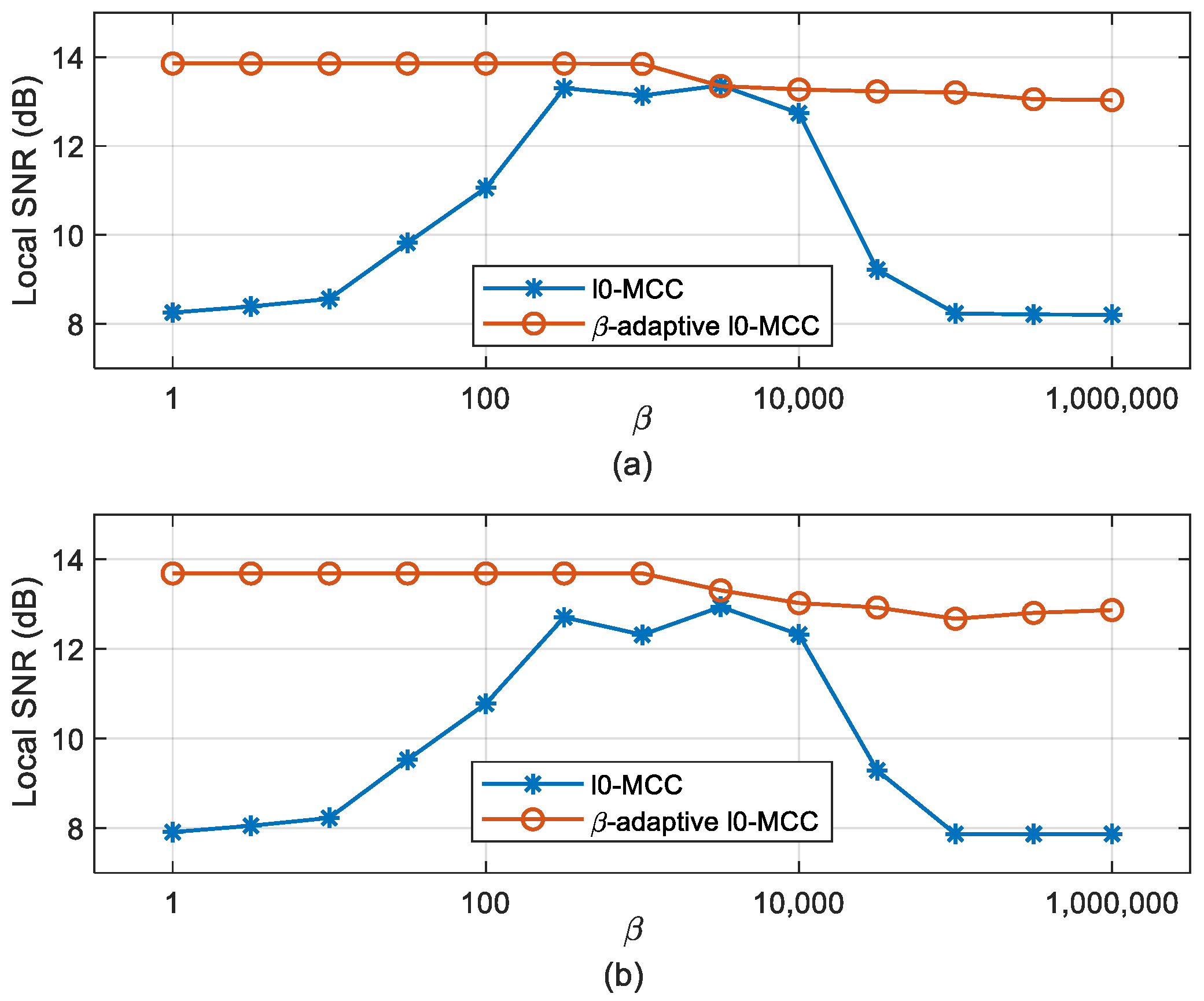
The sensitivity of β was also analyzed. β was set to a wide range, from 1 to 10⁶. The local SNR of ALE output under different values of β is compared, and the results are shown in Figure 7. The performance of l₀-MCC-ALE drops close to 6 dB when β is too large or too small, but β-adaptive l₀-MCC-ALE always maintains good performance. The simulation results show that β-adaptive l₀-MCC-ALE effectively reduces the sensitivity of parameter β, which makes the implementation of the ALE simpler and more reliable.

5. Experiment

To further verify the proposed ALE, the sea trial data were collected in the South China Sea during the summer of 2022. The sea depth was about 130 m, and the sea state was very smooth (code 1). An ultra-low frequency transmitting transducer was carried by an anchored ship to transmit two single-frequency signals of 21 Hz and 23 Hz. The depth of the transducer was 15 m. At a distance of about 7 km to the east, the underwater acoustic signal is received using a single hydrophone at a depth of 15 m. The received data were processed by the conventional ALE, l₀-MCC-ALE, and β-adaptive l₀-MCC-ALE, respectively. ALE parameters were consistent with those in the simulation above.

The lofargrams of different methods are shown in Figure 8, and the estimated local SNR is shown in

Table 3. Local SNR of lines obtained by different methods. (Experiment).

Enhancement Method	Local SNR of 21 Hz (dB)	Local SNR of 23 Hz (dB)
Original signal	−5.4	−2.6
Conventional ALE	3.5	5.6
l0-MCC-ALE	10.9	13.2
Al0-MCC-ALE	10.9	13.6

. From the lofargrams, it can be seen that there are strong and complex interferences in real marine environments. Results show that the performance of the proposed ALE is much better. The local SNR of β-adaptive l₀-MCC-ALE output is more than 7 dB higher than that of conventional ALE. Figure 9 shows the variation of the local SNR with the input parameter β. It can be seen that β-adaptive l₀-MCC-ALE maintains good performance when β changes in a wide range. This means that we no longer need to focus on the appropriate value of β, which simplifies the selection of parameter β.

6. Conclusions

In this paper, a β-adaptive l₀-MCC-ALE is proposed for passive sonars to enhance lines in radiated noise. On the one hand, inspired by the sparsity of lines in the frequency domain, ALE is constrained by the l₀ norm to update the weight vector in the frequency domain. By making the frequency response of ALE sparser, the steady-state misalignment of conventional ALE is reduced, and the SNR of lines is further improved. On the other hand, MCC is used to replace the cost function of LMS, overcoming the defect that conventional ALE is under the assumption of white noise, which makes it more suitable for the colored background noise of real marine environments. In addition, to solve the problem that the performance is sensitive to the parameter β, a β-adaptive method is proposed to keep β in a proper range during iteration. Simulation results show that the proposed ALE has a strong line enhancement ability, and the local SNR of lines is improved by about 8 dB compared with conventional ALE. The value of β is insensitive to its performance, which effectively reduces the cost of selecting β. The results of sea trial data processing also verify the validity of the proposed ALE. In the face of powerful and complex real environment interference, the proposed ALE still has excellent performance.