An Efficient Transmitter Feature Extraction Scheme with IQ Imbalance and Nonlinearity in TDD OFDM Systems

Abstract

Radio frequency (RF) fingerprints have been an emerging research topic for the last decade. Numerous algorithms for recognition have been proposed. However, very few algorithms for the accurate extraction of IQI and PA nonlinearity are available, especially when multiple paths are considered. In this study, we present a scheme that uses the transmitter in-phase/quadrature-phase imbalance (IQI) and the power amplifier (PA) nonlinearity as RF fingerprint features in time-division duplexing (TDD) OFDM systems, which are always considered to be harmful to data transmission. The scheme consists of two round trips with four steps for two cases: in the first, the IQI and PA nonlinearity are unknown at the terminal; in the second, they are known at the terminal. A channel state information (CSI)-tracking algorithm based on the sliding-window least squares method is first adopted at the terminal. In case A, the obtained CSI is sent to the base station (BS) to remove its impact there; in case B, this removal is conducted directly by using pre-equalization at the terminal. Then, by following a sequential iterative approach, the IQI and nonlinearity are individually calculated. Theoretical analyses reveal how CSI estimation errors influence subsequent estimates at the BS in these two cases. Furthermore, the approximate unbiasedness is verified. The theoretical variance and Cramer–Rao lower bound (CRLB) are also given. It is indicated that the theoretical minimum variance in case B is lower than that in case A from the perspective of the CRLB. The numerical results demonstrate the efficiency of the scheme in comparison with existing techniques in the literature.

1. Introduction

With the development of B5G and 6G communication technologies, the physical-layer security of communication is becoming increasingly important, not only for future mobile communication systems but also for the internet of things (IoT) [1,2,3]. Security mechanisms that do not need to be built by using cryptography-based means in the upper layers and that rely solely on inherent physical-layer characteristics have their own unique characteristics, such as the inherent fingerprints of electronic components in transmitters, design defects or vulnerabilities in components in circuits, and the open propagation of electromagnetic waves in wireless communications [4]. In-phase/quadrature-phase imbalance (IQI) and power amplifier (PA) nonlinearity are two key transmitter characteristics that are relatively stable over the long term and vary from device to device [5,6]. They are harmful for data transmission, but are unique to each transmitter for use as a radio frequency (RF) fingerprint. Therefore, it is intuitive to use the transmitter IQI and PA nonlinearity as the RF fingerprint of a transmitter.

IQI estimation is always found in the field of channel equalization and is used to compensate for the distortion of the received signal generated by the IQI. A large number of methods based on linear technology have already been extensively discussed. In [7,8], Alireza Tarighat proposed the least squares (LS) and adaptive equalization method for estimating the combination of transmitter and receiver IQI and channel state information (CSI) to compensate for the resulting transceiver performance degradation. The CSI and IQI were independently estimated based on the pilot by using linear estimation technology in a multiuser single-input–multiple-output (MU-SIMO) system; first, the linear minimum mean squared error (LMMSE) was used to estimate the CSI, and then LS was used to estimate the IQI, thus achieving the separation of the CSI and IQI parameters due to the assumption of IQI at the receiver only [9]. The transmitter (TX) and receiver (RX) IQI compensation problem in differential space–time block-coded orthogonal frequency division multiplexing (STBC-OFDM) systems was studied in [10] and developed further in [11]; the TX and RX IQIs were extracted by employing an algorithm based on a widely linear estimation. An iterative decision feedback (DFB) receiver was proposed to compensate for the IQI due to imperfections in the transceiver RF link for a single carrier with a frequency-domain equalization (SC-FDE) system [12]. This method was a nonlinear compensation method that could greatly improve the equalization performance of an SC-FDE system under IQI compared to the above-mentioned approaches. The authors of [13] used an iterative nonlinear least squares (NLS) method to jointly estimate the IQI in the TX, RX, and channels for generalized orthogonal frequency-division multiplexing (GFDM) systems. Ayse Elif Canbilen [14] investigated the impact of the IQI under generalized Beckmann fading channels for SM-MIMO systems, and both TX and RX IQIs were involved. A performance analysis of the effective channel estimation (e.g., the joint effect of the IQI and channel) and MMSE-based estimation was conducted in [15,16], where the RX IQI was considered in uplink MIMO-OFDM systems. Xiantao Cheng addressed two similar algorithms for estimating the IQI and CSI. One was a sequential estimation algorithm for determining the transmitter IQI and CSI [17], and the other was an EM-based estimation algorithm for determining the transceiver IQI and CSI [18]. Unlike previous methods, they were able to obtain separate estimates of the IQI and CSI. However, our simulation studies showed that these algorithms tended to fall into local minima.

The various methods mentioned above are able to effectively combat performance degradation due to IQI in direct conversion systems, but none of them take the PA nonlinearity of the transmitter into account. PA nonlinearity exists at the front-end of an RF link, and it distorts digitally modulated signals in wireless communications [19,20]. In addition to in-band distortion, the spectral regrowth of digitally modulated signals and adjacent channel interference are also produced by PA nonlinearity [19,20]. PA nonlinearity and IQI are always exploited in specific emitter identification (SEI) (also known as RF-distinct native attribute (RF-DNA) fingerprints) due to their uniqueness and long-term invariant nature [4].

In [21], Ming-Wei Liu extracted PA nonlinearity by using an alternate iterative LS estimation of the channel coefficients and distorted baseband signal to obtain this reliable characteristic in a transmitter based on a training sequence. However, this algorithm required a certain number of samples with a low-enough amplitude in the sequence; otherwise, severe performance degradation would be inevitable. Recently, many works have employed machine learning technology, such as classification algorithms and deep learning technology, to cope with SEI [5,6,22,23]. In such works, a number of simulated and practical trials were conducted, thus verifying the efficiency and reliability of their proposed methods. Nevertheless, unlike traditional approaches [7,8,9,10,11,12,13,14,15,16,17,18], machine learning is powerless in environments without samples, due to its requirements for learning.

In a word, in the previous literature, there are almost no algorithms that directly extract these two transmitter features separately, especially in the presence of multiple paths. The contributions of this study are summarized as follows:

• We establish a feature model of the IQI and PA nonlinearity at the transmitter with multiple paths. Following a brief analysis, we reveal that it is not possible to separately extract the parameters from just one transmission. However, separately extracting IQI and PA nonlinearity under the impact of the CSI is necessary for robust feature extraction. To this end, we propose a scheme for separately estimating the IQI and PA nonlinearity, which involves two round trips with four steps.
• The CSI is estimated/tracked via a sliding-window LS algorithm based on previously depicted training sequences in the first round trip. Then, the IQI and PA nonlinearity of the transmitter are obtained by utilizing a sequential iterative approach after removing the impact of the CSI in the second round trip. The scheme includes two cases: A: IQI and PA nonlinearity are unknown at the terminal; B: IQI and PA nonlinearity are known at the terminal. These have different procedures in steps 3 and 4. The terminal needs to send the coded CSI to the base station (BS) in order to eliminate the channel effect at the BS for case A. The latter deals with the channel effect directly via pre-equalization in step 3 so as to estimate the IQI and PA nonlinearity more simply at the BS for case B.
• We also derive the performance expressions for the two cases and indicate the influence of CSI estimation/tracking. The results of the theoretical analysis show that the theoretical minimum variance in case B is lower than that in case A from the perspective of the Cramer–Rao lower bound (CRLB). In addition, the results of a numerical simulation verify the efficiency of the proposed scheme.

The rest of this study is organized as follows: We first describe the system model and give a CSI tracking algorithm based on the sliding-window LS (CTA_SWLS) with the IQI at the receiver of a terminal in Section 2.  In Section 3, we propose an efficient scheme, with four steps, for eliminating the channel impact, and a sequential iterative approach for simultaneously and separately estimating the TX IQI and nonlinear coefficient at the BS is given. This is followed by a performance analysis and an analysis of the CRLB and complexity of the proposed scheme with the two cases in Section 4. Section 5 demonstrates the simulation results. Finally, conclusions are given in Section 6.

Notation: ${(•)}^{*}$, ${(•)}^T$, and ${(•)}^H$ denote the complex conjugate, transpose, and complex conjugate transpose, respectively. ⊙ denotes element-by-element multiplication. ∗ represents circular convolution. DFT{x} and IDFT{X} denote the discrete Fourier transform of x and the inverse discrete Fourier transform of X, respectively. X mod Y refers to taking the remainder after the division of X by Y. Imaginary units are represented by j. Re{X} and Im{X} denotes taking the real part and imaginary part of X, respectively. $\frac{{\mathbf{X}}_{•}}{\mathbf{Y}}$ indicates element-by-element division. The subscript or superscript i or k indicates the index of a variable, vector, or matrix in its context. $\frac{\partial \Im }{\partial x_0}={\left.\frac{\partial \Im }{\partial x}\right|}_{x=x_0}$ refers to taking the partial derivative of ℑ with respect to x when $x=x_0$.

2. System Model and Analysis

Here, we consider a direct upconversion transmitter in which the carrier frequency from an oscillation source is $f_c$, the phase difference between the I-branch and Q-branch is 90 degrees, and the amplitude coefficients are equal under ideal conditions. However, due to imperfections in the components of the analog circuits in the transmitter RF link and the diversity in manufacturing, the phases of the two branches do not have a difference of strictly 90 degrees, and the amplitude coefficients are not strictly the same, resulting in errors in the demodulated data on the receiver side if there is no countermeasure. On the other hand, the nonlinearity of the transmitter PA also leads to performance degradation at the receiver.

We assume here that no IQI and PA linearity are maintained across the operating range at the BS. Generally speaking, the BS has a more powerful function and can use higher-cost wide-linearity-region PA- and IQI-free devices; IQI and nonlinearity are even present in the RF link, which can also be pre-corrected to achieve more perfect IQ balance and PA linearity, while this is more difficult to achieve at the terminals due to the relatively low cost and performance of the devices, as well as the relatively large number of terminals.

2.1. TX IQI at the Terminal Only

Let $d\left(t\right)=d_I\left(t\right)+j{d}_Q\left(t\right)$ denote the ideal baseband equivalence symbol of the transmitter link at the terminal OFDM system. Because of the impact of the TX IQI at the terminal, this signal is distorted into the following form:

$$s\left(t\right)=ud\left(t\right)+v{d}^{*}\left(t\right),$$

(1)

where u and v are the TX IQI coefficients, which are defined by the following two equations:

$$\begin{array}{c}\hfill u=cos(\theta /2)+j\alpha sin(\theta /2)\\ \hfill v=\alpha cos(\theta /2)+jsin(\theta /2),\end{array}$$

(2)

where $\alpha$ and $\theta$ are the amplitude imbalance and the phase imbalance, respectively, generated by the same local oscillator; this is called a symmetric IQI model. As shown in Figure 1a, under conditions of no IQI, $u=1$ and $v=0$.

Considering that the OFDM system consists of N subcarriers, the symbol period is T, $T=N{T}_s$, the cyclic prefix is $N_{cp}$, and $T_s$ denotes the sampling period. The discrete signal expressions in the following parts of this study are all normalized by the sampling period unless specifically stated. The uplink signal received by the BS is

$$r\left(n\right)=\left[ud\left(n\right)+v{d}^{*}\left(n\right)\right]\ast h\left(n\right)+w\left(n\right),$$

(3)

where $h\left(n\right)$ is the multipath channel length of L, and $w\left(n\right)$ is additional white Gaussian noise (AWGN).

2.2. CSI Estimation with the RX IQI at the Terminal

If we consider the RX IQI at the terminal, a high-frequency (HF) signal that is received passes through a bandpass filter (BPF) and enters a low-noise amplifier (LNA), whose function is mainly to increase the output signal-to-noise ratio (SNR) (unlike the PA), so it can be considered linear over the entire operation range, as shown in Figure 1b. To facilitate the illustration of estimating the CSI at the terminal, we use an asymmetric model to describe the received signal in this section [9,24]. Thus, the signal received at the terminal in the time-division duplexing (TDD) system is

$$\begin{array}{c}\hfill y_{down\_r}\left(n\right)={\beta }_1[d_B\left(n\right)\ast h\left(n\right)+w_{dwon\_r}\left(n\right)]+{\beta }_2[d_B^{*}\left(n\right)\ast h^{*}\left(n\right)+w_{down\_r}^{*}\left(n\right)],\end{array}$$

(4)

where $d_B\left(n\right)$ represents a training sequence sent by the BS to the terminal, $w_{dwon\_r}\left(n\right)$ is AWGN, and $w_{dwon\_r}\left(n\right)\sim \mathcal{CN}(0,{\sigma }_{w_{down\_r}}^2)$. ${\beta }_1=\frac{1+g{e}^{j{\theta }^{\prime }}}{2}$ and ${\beta }_2=\frac{1-g{e}^{-j{\theta }^{\prime }}}{2}$ are the RX IQI coefficients. Their complementary property is ${\beta }_1+{\beta }_2^{*}=1$, and this can be exploited to separate the received signal and the RX IQI. By taking the conjugate to (4) and adding it, we obtain

$$\begin{array}{c}\hfill y_{down\_r}\left(n\right)+y_{down\_r}^{*}\left(n\right)=d_B^{*}\left(n\right)\ast h^{*}\left(n\right)+d_B\left(n\right)\ast h\left(n\right)+w_{down\_r}\left(n\right)+w_{down\_r}^{*}\left(n\right).\end{array}$$

(5)

Let $\mathrm{DFT}\left\{x\right(n\left)\right\}=X\left(k\right)$, which satisfies the conjugate symmetry $\mathrm{DFT}\left\{x^{*}\left(n\right)\right\}=X^{*}(N-k)$. Taking the DFT of (5) and using conjugate symmetry and the complementary property results in

$$\begin{array}{c}\hfill \left\{\begin{array}{c}{Y}_{down\_r}\left(k\right)+Y_{down\_r}^{*}(N-k)\hfill \\ =D_B\left(k\right)H\left(k\right)+D_B^{*}(N-k)H^{*}(N-k)\hfill \\ +W_{down\_r}\left(k\right)+W_{down\_r}^{*}(N-k)1\le k\le \frac{N}{2}-1\hfill \\ \mathrm{Re}\left\{Y_{down\_r}\left(k\right)\right\}\hfill \\ =\mathrm{Re}\{D_B\left(k\right)H\left(k\right)+W_{down\_r}\left(k\right)\}k=0,\frac{N}{2}.\hfill \end{array}\right.\end{array}$$

(6)

It can be seen in (6) that when sending $P(P\ge 2)$ different training sequences, we can obtain $\frac{N}{2}+1$ independent linear equations; each equation can estimate two variables of the CSI via the LS. However, considering the time-varying nature of wireless channels, P sequences are required to be no longer than the channel coherence time [25].

$$P(T+T_{cp})<T_c=\frac{0.423}{f_m},$$

(7)

where $f_m$ is the Doppler shift. For better tracking performance within the channel coherence time, we can send P consecutive but different training sequences circularly, herein utilizing the sliding-window LS algorithm to estimate the CSI for each symbol period. We introduce the symbol period index i and rewrite (6) in matrix form, resulting in

$$\begin{array}{c}\hfill {\mathbf{A}}_k^i{\mathbf{H}}_k^i+{\mathbf{W}}_k^i=[{\mathbf{A}}_{k1}^i,{\mathbf{A}}_{k2}^i]{\mathbf{H}}_k^i+{\mathbf{W}}_k^i={\mathbf{Y}}_k^{i}P\le i,0\le k\le \frac{N}{2},\end{array}$$

(8)

where

$$\begin{array}{c}\hfill {\mathbf{A}}_{k1}^i=\left\{\begin{array}{c}[D_{B,(i-P+1)modP}\left(k\right),D_{B,(i-P+2)modP}\left(k\right),\dots ,\hfill \\ D_{B,imodP}{\left(k\right)]}^{T}P\le i,1\le k\le \frac{N}{2}-1\hfill \\ 2[\mathrm{Re}\left\{D_{B,(i-P+1)modP}\left(k\right)\right\},\mathrm{Re}\left\{D_{B,(i-P+2)modP}\left(k\right)\right\},\dots ,\hfill \\ \mathrm{Re}\left\{D_{B,imodP}\left(k\right)\right\}{]}^{T}P\le i,k=0,\frac{N}{2},\hfill \end{array}\right.\end{array}$$

(9)

$$\begin{array}{c}\hfill {\mathbf{A}}_{k2}^i=\left\{\begin{array}{c}[D_{B,(i-P+1)modP}^{*}(N-k),D_{B,(i-P+2)modP}^{*}(N-k),\dots ,\hfill \\ D_{B,imodP}^{*}{(N-k)]}^{T}P\le i,1\le k\le \frac{N}{2}-1\hfill \\ 2[-\mathrm{Im}\left\{D_{B,(i-P+1)modP}\left(k\right)\right\},-\mathrm{Im}\left\{D_{B,(i-P+2)modP}\left(k\right)\right\},\dots ,\hfill \\ -\mathrm{Im}\left\{D_{B,imodP}\left(k\right)\right\}{]}^{T}P\le i,k=0,\frac{N}{2},\hfill \end{array}\right.\end{array}$$

(10)

$$\begin{array}{c}\hfill {\mathbf{H}}_k^i=\left\{\begin{array}{c}{[H^i\left(k\right),{H^i}^{*}(N-k)]}^{T}P\le i,1\le k\le \frac{N}{2}-1\hfill \\ {[\mathrm{Re}\left\{H^i\left(k\right)\right\},\mathrm{Im}\left\{H^i\left(k\right)\right\}]}^{T}P\le i,k=0,\frac{N}{2},\hfill \end{array}\right.\end{array}.$$

(11)

$$\begin{array}{cc}\hfill {\mathbf{Y}}_k^i=& [Y_{down\_r,(i-P+1)}\left(k\right)+Y_{down\_r,(i-P+1)}^{*}(N-k),\hfill \\ & Y_{down\_r,(i-P+2)}\left(k\right)+Y_{down\_r,(i-P+2)}^{*}(N-k),\dots ,\hfill \\ & Y_{down\_r,i}\left(k\right)+Y_{down\_r,i}^{*}{(N-k)]}^{T}P\le i,0\le k\le \frac{N}{2},\hfill \end{array}.$$

(12)

$$\begin{array}{cc}\hfill {\mathbf{W}}_k^i=& [W_{down\_r,(i-P+1)}\left(k\right)+W_{down\_r,(i-P+1)}^{*}(N-k),\hfill \\ & W_{down\_r,(i-P+2)}\left(k\right)+W_{down\_r,(i-P+2)}^{*}(N-k),\dots ,\hfill \\ & W_{down\_r,i}\left(k\right)+W_{down\_r,i}^{*}{(N-k)]}^{T}P\le i,0\le k\le \frac{N}{2}.\hfill \end{array}$$

(13)

It is easy to obtain the CSI estimate as follows:

$${\widehat{\mathbf{H}}}_k^i={\left({\mathbf{A}}_k^{iH}{\mathbf{A}}_k^i\right)}^{-1}{\mathbf{A}}_k^{iH}{\mathbf{Y}}_k^{i}P\le i,0\le k\le \frac{N}{2}.$$

(14)

Since interchanges of rows or columns of a matrix do not change its singular values, ${\left({\mathbf{A}}_k^{iH}{\mathbf{A}}_k^i\right)}^{-1}={\left({\mathbf{A}}_k^H{\mathbf{A}}_k\right)}^{-1}$ is a fixed value. Let

$$\begin{array}{c}\hfill {\mathrm{Y}}_k^i={\mathbf{A}}_k^{iH}{\mathbf{Y}}_k^i={\mathrm{Y}}_k^{i-1}+{\mathbf{A}}_k{\left(imodP\right)}^H[{\mathbf{Y}}_k^i(P-1)-{\mathbf{Y}}_k^{i-1}\left(0\right)]P\le i,\end{array}.$$

(15)

Thus,

$${\widehat{\mathbf{H}}}_k^i={\widehat{\mathbf{H}}}_k^{i-1}+{\left({\mathbf{A}}_k^H{\mathbf{A}}_k\right)}^{-1}{\mathrm{Y}}_k^{i}P\le i,0\le k\le \frac{N}{2},$$

(16)

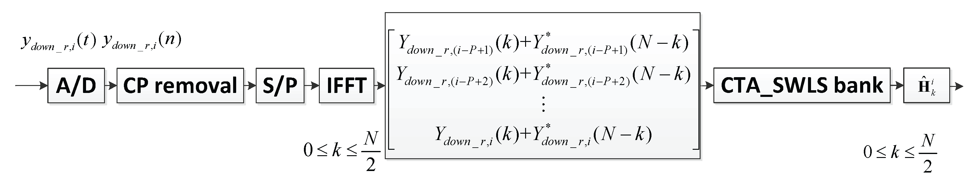
where ${\mathbf{A}}_k\left(i\right)$ denotes row $i+1$ of ${\mathbf{A}}_k$, as well as ${\mathbf{Y}}_k^i\left(i\right)$. To avoid large estimation errors, it is necessary to design the training sequences with a small condition number for ${\mathbf{A}}_k$. The CSI tracking algorithm based on the sliding window LS (CTA_SWLS) is given in the form of Algorithm 1 and is shown in Figure 2.

Algorithm 1 CSI tracking algorithm based on the sliding-window LS (CTA_SWLS).

1: Initial $i=P-1$; Calculate ${\mathbf{B}}_k={\left({\mathbf{A}}_k^H{\mathbf{A}}_k\right)}^{-1}$ and ${\widehat{\mathbf{H}}}_k^i={\mathbf{B}}_k{\mathbf{A}}_k^{iH}{\mathbf{Y}}_k^i$ offline. 2: For $i\ge P$    Calculate ${\mathrm{Y}}_k={\mathbf{A}}_k{\left(imodP\right)}^H[{\mathbf{Y}}_k^i(P-1)-{\mathbf{Y}}_k^{i-1}\left(0\right)]$;    Update ${\widehat{\mathbf{H}}}_k^i={\widehat{\mathbf{H}}}_k^{i-1}+{\mathbf{B}}_k{\mathrm{Y}}_k$;    $i=i+1$ End

2.3. TX Link with Nonlinear PA Only at the Terminal

Considering a memoryless PA, via Taylor expansions, a complex power-series expansion can be used to model the effect of a digital baseband signal passing through a transmitter front-end PA [20,21]. Accordingly, the even terms of the expanded series are discarded, leaving only the odd items, such that the baseband signal becomes

$$x=\sum _{i=0}^{M-1}{b}_m{d}^{m+1}(d^{*}{)}^m=\sum _{i=0}^{M-1}{b}_m{\left|d\right|}^{2m}d.$$

(17)

In (17), x denotes the signal after the baseband signal d passes the nonlinear PA, and $b_m$ is a complex coefficient of odd items. Equation (17) shows that the items of $m=0$ form the linear component of the PA. To facilitate analysis, herein, let $b_m$ be normalized to $b_0$, so $b_0=1$. We rewrite (17) in matrix form as follows:

$$\mathbf{x}=[\mathbf{d},{\mathbf{D}}_1]\mathbf{b}=\mathbf{Db},$$

(18)

where $\mathbf{x}={[x_0,x_1,\dots ,x_{N-1}]}^T$, $\mathbf{d}={[d_0,d_1,\dots ,d_{N-1}]}^T$, ${\left[\mathbf{D}\right]}_{i,m}={\left|d_i\right|}^{2m}$ and $\mathbf{b}={[b_0,\dots ,b_{M-1}]}^T$.

2.4. Coexistence of the TX IQI and PA Nonlinearity in the Terminal Transmitter Link

By combining the IQ imbalance and PA nonlinearity and considering multipath channels and noise, the following received signals can be obtained at the BS:

$$\mathbf{r}=\mathbf{x}\ast \mathbf{h}+\mathbf{n}=\left([\mathbf{s},{\mathbf{S}}_R]\mathbf{b}\right)\ast \mathbf{h}+\mathbf{n}=\left(\mathbf{Sb}\right)\ast \mathbf{h}+\mathbf{n},$$

(19)

where $\mathbf{s}$ is the first column of $\mathbf{S}$, and ${\mathbf{S}}_R$ is a matrix whose columns are composed of the last $M-1$ columns of $\mathbf{S}$. $\mathbf{n}$ is an additional white Gaussian noise (AWGN) vector, and $\mathbf{n}\sim \mathcal{CN}(0,{\sigma }^2{\mathbf{I}}_{N\times N})$. Thus, matrix $\mathbf{S}$ becomes ${\left[\mathbf{S}\right]}_{i,m}={\left|u{d}_i+v{d}_i^{*}\right|}^{2m}(u{d}_i+v{d}_i^{*})$.

It can be seen from $\mathbf{S}$ that the IQI coefficients u and v are in each element of $\mathbf{S}$, as well as in the nonlinearity coefficient vector $\mathbf{b}$; all of these are the transmitter features that need to be extracted. If the CSI is unknown at the BS, an arbitrary set of values of u and v can be used to determine the matrix $\mathbf{S}$ by combining arbitrary values of $\mathbf{b}$, provided that $\mathbf{h}$ takes an appropriate value; this can make (19) consistent whether there is error or not. Hence, the parameters in this model cannot be determined if the CSI is unknown at the BS. With special cases in which $b_0=1$, $b_m=0 (m>0)$, which is a scenario that has been extensively studied in many previous papers [7,8,9,10,11,12,13,14,15,16,17,18]. However, for transmitter feature extraction, the requirement of obtaining independent estimates of the transmitter IQ imbalance and PA nonlinearity from multiple paths is necessary. Therefore, we need to seek a new approach to deal with this issue.

The situation will be different under the condition that the CSI is known according to (19). If a set of values of u and v are available, by using LS estimation, an estimate of $\mathbf{b}$ can be obtained; the closer the values of u and v are to their true values in all estimates, the more accurate the estimate of $\mathbf{b}$ is in the sense of the LS. Note that the LS algorithm requires that the column rank of $\mathbf{s}$ be equal to the number of non-zero terms in $\mathbf{b}$; otherwise, it will be ill conditioned, leading to large errors. Since $\mathbf{S}$ can be written as

$$\mathbf{S}=\mathrm{diag}(\mathbf{s})\mathrm{\Psi },$$

(20)

where ${\left[\mathrm{\Psi }\right]}_{i,m}={\left|u{d}_i+v{d}_i^{*}\right|}^{2m}$ is a Vandermonde matrix, $\mathrm{rank}\left(\mathbf{S}\right)\le min\left\{\mathrm{rank}\right(\mathrm{diag}\left(\mathbf{s}\right)),\mathrm{rank}(\mathrm{\Psi }\left)\right\}$ is equal to a non-zero number, and the rank of $\mathrm{\Psi }$ is equal to the number of different non-zero $d_i$ values. In other words, the number of different non-zero $d_i$ values in the training sequence is greater than the number of non-zero elements of $\mathbf{b}$. $\mathbf{b}$ has an LS solution for the existence of IQI. Nevertheless, for IQI-free cases, the rank of $\mathrm{\Psi }$ is determined by the number of different non-zero $\left|d_i\right|$ values. It is, therefore, necessary that the number of different amplitudes is not less than M.

3. The Proposed Scheme

The above analysis shows that when the CSI is unknown at the BS, the model has no deterministic solution. Therefore, we propose a scheme for the joint and independent extraction of the IQI and nonlinear parameters in the terminal transmitter, and this scheme has two cases, which are shown in Figure 3.

3.1. Case A: IQI and PA Nonlinearity Are Unknown at the Terminal

In this case, transmitter feature extraction and authentication are conducted via two round trips with four steps in TDD systems.

Step 1: The terminal sends an access request to the BS.

Step 2: Upon receipt of the request by the BS, P consecutive but different training sequences are cyclically sent to the terminal.

Step 3: The CTA_SWLS algorithm is employed to track the CSI after P training sequences are received at the terminal. When ${\displaystyle \sum _{k=0}^{N/\phantom{N2}2}}{∥{\widehat{\mathbf{H}}}_k^i-{\widehat{\mathbf{H}}}_k^{i-1}∥}^2<\delta$ is satisfied ($\delta$ denotes a threshold), an FFT is performed on ${\widehat{\mathbf{H}}}^i$ to obtain the time-domain CSI ${\widehat{\mathbf{h}}}^i$. The first L ( $L>\frac{{\tau }_{max}}{T_s}$ is the max delay spread) values of ${\widehat{\mathbf{h}}}^i$ are retained. Then, a training sequence is sent, and the CSI is truncated to the BS. It is assumed that the CSI remains constant during the last symbol period in step 2 and step 3. Note that to maintain the relevance of the CSI, the training sequence needs to be sent to the BS before the CSI.

Step 4: The BS estimates the combination of the CSI and transmitter IQI based on the training sequence in step 3 by using the LS or MMSE with PA nonlinearity; then, it demodulates the data, which are also known as the CSI. Followed by the removal of the effect of the CSI in the received signal, the BS then estimates the terminal IQI and PA nonlinearity coefficients. The features are stored in a local database either directly or after processing. It is also possible to compare data in the database by using pattern recognition so that the resulting signal to accept or reject the transmitter’s access can be given.

Considering the effects of PA nonlinearity and noise, in step 3, when the terminal encodes and modulates the estimated CSI, it should use a lower-order modulation method, such as BPSK or QPSK, on each OFDM subcarrier. For example, the number of effective paths is generally within 10 for a frequency-selective channel; when using 10 bits (1024-level uniform quantization) and BPSK modulation, a total of 100 bits are required. As long as the number of subcarriers satisfies $N\ge 100$, this requirement is met. After the BS receives the CSI and removes the impact of the channel, Equation (19) becomes

$${\mathbf{r}}^{\mathsf{\prime }}=\mathbf{Sb}+{\mathbf{n}}^{\mathsf{\prime }},$$

(21)

where ${\mathbf{r}}^{\mathsf{\prime }}=\frac{1}{\sqrt{N}}{\mathbf{F}}^H\frac{{\mathbf{Fr}}_{•}}{\mathbf{F}{\mathbf{h}}_0}$ and ${\mathbf{n}}^{\mathsf{\prime }}=\frac{1}{\sqrt{N}}{\mathbf{F}}^H\frac{{\mathbf{Fn}}_{•}}{\mathbf{F}{\mathbf{h}}_0}$. ${\left[\mathbf{F}\right]}_{k,n}=\frac{1}{\sqrt{N}}{e}^{-j2\pi nk/N}$ is a Fourier matrix. This problem now turns into

$$\begin{array}{c}\underset{u,v,b}{min}{∥{\mathbf{r}}^{\mathsf{\prime }}-\mathbf{Sb}∥}^2\hfill \\ s.t.b_0=1.\hfill \end{array}$$

(22)

Let $\mathbf{\nu }={(\mathbf{b},u,v)}^T$. Since u and v in $\mathbf{S}$ are to be estimated, $\mathbf{b}$ is also to be estimated; we use a sequential iterative approach to estimate these quantities.

Setting the initial values to $u=1$ and $v=0$, first, we calculate

$${\widehat{\mathbf{b}}}^{\mathsf{\prime }}={\left({{\mathbf{S}}_R}^H{\mathbf{S}}_R\right)}^{-1}{{\mathbf{S}}_R}^H({\mathbf{r}}^{\mathsf{\prime }}-\mathbf{s}),$$

(23)

where $\widehat{\mathbf{b}}={[1,{\widehat{\mathbf{b}}}^{\mathsf{\prime }}]}^T$. Next, by utilizing the gradient descent method, the estimate of v can be iteratively obtained as follows:

$$\begin{array}{cc}\hfill \widehat{v}& =\widehat{v}-\mu \frac{\partial {∥{\mathbf{r}}^{\mathsf{\prime }}-\mathbf{S}\widehat{\mathbf{b}}∥}^2}{\partial v}\hfill \\ \hfill & =\widehat{v}-\mu (\frac{\partial ({\widehat{\mathbf{b}}}^H{\mathbf{S}}^H\mathbf{S}\widehat{\mathbf{b}}-{{\mathbf{r}}^{\mathsf{\prime }}}^H\mathbf{S}\widehat{\mathbf{b}}-{\widehat{\mathbf{b}}}^H{\mathbf{S}}^H{\mathbf{r}}^{\mathsf{\prime }})}{\partial v_x}\hfill \\ & -j\frac{\partial ({\widehat{\mathbf{b}}}^H{\mathbf{S}}^H\mathbf{S}\widehat{\mathbf{b}}-{{\mathbf{r}}^{\mathsf{\prime }}}^H\mathbf{S}\widehat{\mathbf{b}}-{\widehat{\mathbf{b}}}^H{\mathbf{S}}^H{\mathbf{r}}^{\mathsf{\prime }})}{\partial v_y}),\hfill \end{array}$$

(24)

where $\mu$ is a small positive value for controlling the step size. In addition,

$$\begin{array}{c}\hfill \frac{\partial ({\widehat{\mathbf{b}}}^H{\mathbf{S}}^H\mathbf{S}\widehat{\mathbf{b}}-{{\mathbf{r}}^{\mathsf{\prime }}}^H\mathbf{S}\widehat{\mathbf{b}}-{\widehat{\mathbf{b}}}^H{\mathbf{S}}^H{\mathbf{r}}^{\mathsf{\prime }})}{\partial v_x}={\widehat{\mathbf{b}}}^H(\frac{\partial {\mathbf{S}}^H}{\partial v_x}\mathbf{S}+{\mathbf{S}}^H\frac{\partial \mathbf{S}}{\partial v_x})\widehat{\mathbf{b}}-{{\mathbf{r}}^{\mathsf{\prime }}}^H\frac{\partial \mathbf{S}}{\partial v_x}\widehat{\mathbf{b}}-{\widehat{\mathbf{b}}}^H\frac{\partial {\mathbf{S}}^H}{\partial v_x}{\mathbf{r}}^{\mathsf{\prime }}\end{array}$$

$$\begin{array}{c}\hfill \frac{\partial ({\widehat{\mathbf{b}}}^H{\mathbf{S}}^H\mathbf{S}\widehat{\mathbf{b}}-{{\mathbf{r}}^{\mathsf{\prime }}}^H\mathbf{S}\widehat{\mathbf{b}}-{\widehat{\mathbf{b}}}^H{\mathbf{S}}^H{\mathbf{r}}^{\mathsf{\prime }})}{\partial v_y}={\widehat{\mathbf{b}}}^H(\frac{\partial {\mathbf{S}}^H}{\partial v_y}\mathbf{S}+{\mathbf{S}}^H\frac{\partial \mathbf{S}}{\partial v_y})\widehat{\mathbf{b}}-{{\mathbf{r}}^{\mathsf{\prime }}}^H\frac{\partial \mathbf{S}}{\partial v_y}\widehat{\mathbf{b}}-{\widehat{\mathbf{b}}}^H\frac{\partial {\mathbf{S}}^H}{\partial v_y}{\mathbf{r}}^{\mathsf{\prime }}\end{array}$$

where

$$\begin{array}{c}\hfill \begin{array}{c}\frac{\partial {\mathbf{S}}_{i,m}}{\partial v_x}={\left(\frac{\partial {\mathbf{S}}_{m,i}^H}{\partial v_x}\right)}^{*}=\frac{\partial {\left|u{d}_i+v{d_i}^{*}\right|}^{2m}(u{d}_i+v{d_i}^{*})}{\partial v_x}={\left|u{d}_i+v{d_i}^{*}\right|}^{2m}[m\frac{2v_x{\left|d_i\right|}^2+u{d_i}^2+u^{*}{d}_i{{}^{*}}^2}{{(u{d}_i+v{d_i}^{*})}^{*}}+{d_i}^{*}],\hfill \end{array}\end{array}$$

(25)

$$\begin{array}{c}\frac{\partial {\mathbf{S}}_{i,m}}{\partial v_y}={\left(\frac{\partial {\mathbf{S}}_{m,i}^H}{\partial v_y}\right)}^{*}=\frac{\partial {\left|u{d}_i+v{d_i}^{*}\right|}^{2m}(u{d}_i+v{d_i}^{*})}{\partial v_y}={\left|u{d}_i+v{d_i}^{*}\right|}^{2m}[m\frac{2v_y{\left|d_i\right|}^2-ju{d_i}^2+j{u}^{*}{d_i}^{*2}}{{(u{d}_i+v{d_i}^{*})}^{*}}+j{d_i}^{*}].\hfill \end{array}$$

(26)

The following relationship of u and v based on (2) is used here to estimate u.

$$u=\sqrt{1-v_y^2}+j\frac{v_x{v}_y}{\sqrt{1-v_y^2}}.$$

(27)

After a finite number of iterations, the temporary suboptimal values of $\widehat{v}$ and $\widehat{u}$ can be obtained. Then, $\widehat{v}$ and $\widehat{u}$ are substituted into (23), and the iterative process is repeated until the stopping criteria are met. We summarize the estimation procedure in Algorithm 2.

Algorithm 2 IQI and nonlinearity sequential estimation algorithm (IQINSEA)

1: Initialization: Set $u=1$, $v=0$, $i=0$, $\mu$, ${\epsilon }_1$, ${\epsilon }_2$ 2: For (external iteration)    Update ${{\widehat{\mathbf{b}}}^{\mathsf{\prime }}}_i$ using (23);    Form ${\widehat{\mathbf{b}}}_i={[1,{{\widehat{\mathbf{b}}}^{\mathsf{\prime }}}_i]}^T$;    If $∥[{\widehat{\mathbf{b}}}_i,{\widehat{v}}_i]-[{\widehat{\mathbf{b}}}_{i-1},{\widehat{v}}_{i-1}]∥<{\epsilon }_2$       Stop and calculate ${\widehat{u}}_i$ using (27)       Output: ${\widehat{\mathbf{\nu }}}_i$.    Else       $k=0$;       For (internal iteration)          Using (24) to update ${\widehat{v}}_{i,k+1}$;          If $∥{\widehat{v}}_{i,k+1}-{\widehat{v}}_{i,k}∥<{\epsilon }_1$             Stop          Else             $k=k+1$;          Endif       End       $i=i+1$;    Endif End

3.2. Case B: IQI and PA Nonlinearity Are Known at the Terminal

Figure 3b demonstrates the procedure for case B. Here, prior knowledge is given at the terminal, and the corresponding processing is different to that in case A. The differences between case a and case B are as follows.

Step 3: The CTA_SWLS algorithm is employed to track the CSI after P training sequences are received at the terminal. When ${\displaystyle \sum _{k=0}^{N/\phantom{N2}2}}{∥{\widehat{\mathbf{H}}}_k^i-{\widehat{\mathbf{H}}}_k^{i-1}∥}^2<\delta$ is satisfied, a modified sequence is directly obtained via a pre-equalization operation and sent to the BS instead of step 3 in case A.

Step 4: The BS receives and estimates the terminal IQI and nonlinear coefficients via Algorithm 2. The subsequent actions are the same as those in case A.

Since we only need to send a pre-equalization training sequence to the BS, case B is more suitable for faster-varying channels. With no CSI effect, the signal received by the BS should be shown as follows:

$${\mathbf{r}}^{\mathsf{″}}=\mathbf{Sb}+\mathbf{n}.$$

(28)

The matrix $\mathbf{S}$ is known at both the terminal and the BS, but due to the CSI there is no unique solution, as described in the previous section. Therefore, we are able to send a pre-equalized training sequence to the BS after the CSI is estimated, and a signal with no CSI effect is equivalently received at the BS. To satisfy

$${\mathbf{r}}^{\mathsf{″}}={\mathbf{S}}^{\mathsf{\prime }}\mathbf{b}\ast \mathbf{h}+\mathbf{n}=\mathbf{Sb}+\mathbf{n},$$

(29)

that is,

$${\mathbf{S}}^{\mathsf{\prime }}\mathbf{b}={\mathbf{F}}^H\mathrm{diag}{\left(\mathbf{H}\right)}^{-1}\mathbf{FSb}=\tilde{\mathbf{r}},$$

(30)

Equation (30) can be written as N independent equations for $d_i$:

$$\begin{array}{c}\hfill \sum _{m=0}^{M-1}{b}_m{\left|u{d}_i+v{d_i}^{*}\right|}^{2m}(u{d}_i+v{d_i}^{*})={\tilde{r}}_i+{\tilde{n}}_{i}0\le i\le N-1\end{array}$$

(31)

or

$$F=\left\{\begin{array}{c}{f}_1={\displaystyle \sum _{m=0}^{M-1}}{Q}^m\mathrm{\Phi }{x}_m-Cx=0\hfill \\ f_2={\displaystyle \sum _{m=0}^{M-1}}{Q}^m\mathrm{\Phi }{y}_m-Cy=0\hfill \end{array}\right.0\le i\le N-1,$$

(32)

where

$$Q={\left|u{d}_i+v{d_i}^{*}\right|}^2$$

$$\begin{array}{c}\hfill \mathrm{\Phi }{x}_m=b{x}_m(u_x{d}_{xi}-u_y{d}_{yi}+v_x{d}_{xi}+v_y{d}_{yi})-b{y}_m(u_x{d}_{yi}+u_y{d}_{xi}-v_x{d}_{yi}+v_y{d}_{xi})\end{array}$$

$$\begin{array}{c}\hfill \mathrm{\Phi }{y}_m=b{y}_m(u_x{d}_{xi}-u_y{d}_{yi}+v_x{d}_{xi}+v_y{d}_{yi})+b{x}_m(u_x{d}_{yi}+u_y{d}_{xi}-v_x{d}_{yi}+v_y{d}_{xi})\end{array}$$

$$Cx=\mathrm{Re}\{{\tilde{r}}_i+{\tilde{n}}_i\}$$

$$Cy=\mathrm{Im}\{{\tilde{r}}_i+{\tilde{n}}_i\}.$$

Equation (31) is a binary nonlinear system of equations with respect to $d_{xi}$ and $d_{yi}$, and the solution can be obtained via the Newton–Raphson method. We omit the subscript i and let $\mathbf{d}={\left[d_x,d_y\right]}^T$ so that we can obtain the following solution:

$${\mathbf{d}}^{k+1}={\mathbf{d}}^k-J{\left({\mathbf{d}}^k\right)}^{-1}F\left({\mathbf{d}}^k\right),$$

(33)

where $J\left(\mathbf{d}\right)=\left[\begin{array}{cc}\frac{\partial f_1}{\partial d_x}& \frac{\partial f_1}{\partial d_y}\\ \frac{\partial f_2}{\partial d_x}& \frac{\partial f_2}{\partial d_y}\end{array}\right]$ is a Jacobian matrix. In addition,

$$\frac{\partial f_1}{\partial d_x}=\sum _{m=0}^{M-1}\left(Q^m\frac{\partial \mathrm{\Phi }{x}_m}{\partial d_x}+m{Q}^{m-1}\frac{\partial Q}{\partial d_x}\mathrm{\Phi }{x}_m\right),$$

in which $f_1$ and $\mathrm{\Phi }{x}_m$ can be simultaneously replaced with $f_2$ and $\mathrm{\Phi }{x}_m$. $d_x$ can be replaced with $d_y$.

$$\begin{array}{c}\hfill \frac{\partial Q}{\partial d_x}=2(u_x{d}_x-u_y{d}_y+v_x{d}_x+v_y{d}_y)(u_x+v_x)\\ \hfill +2(u_x{d}_y+u_y{d}_x-v_x{d}_y+v_y{d}_x)(u_y+v_y)\end{array}$$

$$\begin{array}{c}\hfill \frac{\partial Q}{\partial d_y}=2(u_x{d}_x-u_y{d}_y+v_x{d}_x+v_y{d}_y)(v_y-u_y)\\ \hfill +2(u_x{d}_y+u_y{d}_x-v_x{d}_y+v_y{d}_x)(u_x-v_x)\end{array}$$

$$\frac{\partial \mathrm{\Phi }{x}_m}{\partial d_x}=b{x}_m(u_x+v_x)-b{y}_m(u_y+v_y)$$

$$\frac{\partial \mathrm{\Phi }{x}_m}{\partial d_y}=b{x}_m(v_y-u_y)-b{y}_m(u_x-v_x)$$

$$\frac{\partial \mathrm{\Phi }{y}_m}{\partial d_x}=b{y}_m(u_x+v_x)+b{x}_m(u_y+v_y)$$

$$\frac{\partial \mathrm{\Phi }{y}_m}{\partial d_y}=b{y}_m(v_y-u_y)+b{x}_m(u_x-v_x).$$

It is also possible to use nonlinear least squares to find the solution for the following optimization problem:

$$min{\left[\sum _{m=0}^{M-1}{b}_m{\left|ud+v{d}^{*}\right|}^{2m}(ud+v{d}^{*})-(\tilde{r}+\tilde{n})\right]}^2.$$

(34)

It is given as

$${\mathbf{d}}^{k+1}={\mathbf{d}}^k-\eta \nabla \left({\mathbf{d}}^k\right),$$

(35)

where $\nabla \left(\mathbf{d}\right)=2J{\left(\mathbf{d}\right)}^{T}F\left(\mathbf{d}\right)$, and $\eta$ is a small positive value for controlling the step size.

This is a system of N independent binary nonlinear equations that can be calculated in parallel at the transmitter side and implemented very quickly. The received signal that is transmitted to the BS can be eliminated from the CSI beforehand to facilitate subsequent processing at the BS. Once it is received by the BS, Algorithm 2 is used to directly estimate the IQI and nonlinear coefficients.

4. Performance Analysis

4.1. Performance Analysis of CTA_SWLS

Let ${\mathbf{H}}_{0k}^i$ represent the true value of ${\mathbf{H}}_k^i$. Thus, the estimated CSI with k and $N-k$ subcarriers is

$$\begin{array}{c}\hfill {\widehat{\mathbf{H}}}_k^i={\left({\mathbf{A}}_k^H{\mathbf{A}}_k\right)}^{-1}\sum _{p=0}^{P-1}\left\{{\mathbf{A}}_k{\left[\right(i-p)modP]}^H\{{\mathbf{A}}_k[(i-p)modP]{\mathbf{H}}_{0k}^{i-p}+{\mathbf{W}}_k(i-p)\}\right\}.\end{array}$$

(36)

Taking the expectation to $\Delta {\widehat{\mathbf{H}}}_k^i={\widehat{\mathbf{H}}}_k^i-{\mathbf{H}}_{0k}^i$ yields

$$\begin{array}{c}\hfill \mathbb{E}[\Delta {\widehat{\mathbf{H}}}_k^i]={\left({\mathbf{A}}_k^H{\mathbf{A}}_k\right)}^{-1}\sum _{p=0}^{P-1}\left\{{\mathbf{A}}_k{\left[\right(i-p)modP]}^H{\mathbf{A}}_k[(i-p)modP](\mathbb{E}\left[{\mathbf{H}}_{0k}^{i-p}\right]-\mathbb{E}\left[{\mathbf{H}}_{0k}^i\right])\right\}.\end{array}$$

(37)

It can be seen from (37) that the unbiasedness of Algorithm 1 depends on the means of the past $P-1$ true CSI. If the CSI is a stationary process over P symbol periods, then $\mathbb{E}[\Delta {\widehat{\mathbf{H}}}_k^i]=0$, that is, Algorithm 1 is unbiased. It is assumed here that the channel is independent and identically distributed (IID), and ${\mathbf{h}}_0^i\sim \mathcal{CN}(\overline{\mathbf{h}},{\sigma }_h^2{\mathbf{I}}_{N\times N})$ for each path; thus, ${\mathbf{H}}_0^i=\mathrm{DFT}\left({\mathbf{h}}_0^i\right)\sim \mathcal{CN}(\overline{\mathbf{H}},N{\sigma }_h^2{\mathbf{I}}_{N\times N})$, where ${\mathbf{h}}_0^i$ and ${\mathbf{H}}_0^i$ denote the true CSI time-domain and frequency-domain vectors, respectively. $\overline{\mathbf{h}}$ and $\overline{\mathbf{H}}$ denote their respective means.

Then, the autocorrelation matrix of the channel error is given in the form of (38):

$$\begin{array}{cc}\hfill & {\mathbf{R}}_k=\mathbb{E}[\Delta {\widehat{\mathbf{H}}}_k^i\Delta \widehat{\mathbf{H}}{{}_k^i}^H]=\underset{\mathrm{I}}{\underbrace{{\left({\mathbf{A}}_k^H{\mathbf{A}}_k\right)}^{-1}\left\{\sum _{p=0}^P{\mathbf{A}}_k{\left(p\right)}^H{\mathbf{A}}_k\left(p\right){\mathbf{A}}_k{\left(p\right)}^H{\mathbf{A}}_k\left(p\right)\right\}{\left({\mathbf{A}}_k^H{\mathbf{A}}_k\right)}^{-1}{\sigma }_k^2+{\sigma }_k^2\mathbf{I}}}\hfill \\ \hfill & \underset{\mathrm{I}\mathrm{I}}{\underbrace{-\left\{{\left({\mathbf{A}}_k^H{\mathbf{A}}_k\right)}^{-1}{\mathbf{A}}_k{[imodP]}^H{\mathbf{A}}_k[imodP]+{\mathbf{A}}_k{[imodP]}^H{\mathbf{A}}_k[imodP]{\left({\mathbf{A}}_k^H{\mathbf{A}}_k\right)}^{-1}\right\}{\sigma }_k^2}}+\underset{\mathrm{I}\mathrm{I}\mathrm{I}}{\underbrace{2{\left({\mathbf{A}}_k^H{\mathbf{A}}_k\right)}^{-1}N{\sigma }_{w_{down\_r}}^2}},\hfill \end{array}$$

(38)

where ${\sigma }_k^2=\left\{\begin{array}{cc}N{\sigma }_h^2\hfill & 1\le k\le \frac{N}{2}-1\\ N{\sigma }_h^2/2\hfill & k=0,\frac{N}{2}\end{array}\right.$. In (38), I is a fixed item, while II is an item with a period P. Both are generated by channel jitter, and III is generated by AWGN.

4.2. Error Propagation

In this subsection, the performance of Algorithm 2 in Step 4 is described. CSI estimation and quantization errors and demodulation errors in case A, as well as errors arising from pre-equalization in case B, are ignored. Before that, consideration of error propagation is necessary. In the scheme, error propagation affects the estimation of the terminal IQI and nonlinear parameters at the BS.

4.2.1. Case A

The received signal at the BS is

$$\mathbf{r}={\mathbf{S}}_0{\mathbf{b}}_0\ast {\mathbf{h}}_0+\mathbf{n}.$$

(39)

After removing the impact of the CSI, $\mathbf{r}$ is now turned into ${\widehat{\mathbf{r}}}^{\mathsf{\prime }}$ in the estimated version of (21). Then, an FFT is implemented on both sides:

$$\begin{array}{cc}\hfill \sqrt{N}\mathbf{F}{\widehat{\mathbf{r}}}^{\mathsf{\prime }}=& \frac{\sqrt{N}{\mathbf{Fr}}_{•}}{\sqrt{N}\mathbf{F}\widehat{\mathbf{h}}}\hfill \\ \hfill =& \frac{\sqrt{N}\mathbf{F}{\mathbf{S}}_0{{\mathbf{b}}_0}_{•}}{\sqrt{N}\mathbf{F}\widehat{\mathbf{h}}}\odot \sqrt{N}\mathbf{F}{\mathbf{h}}_0+\frac{\sqrt{N}{\mathbf{Fn}}_{•}}{\sqrt{N}\mathbf{F}\widehat{\mathbf{h}}}\hfill \\ \hfill =& \left(\frac{{\mathbf{1}}_{•}^{\circ }}{{\mathbf{1}}^{\circ }+\mathbf{F}\Delta \mathbf{h}/\mathbf{F}{\mathbf{h}}_0}\right)\odot \sqrt{N}\mathbf{F}{\mathbf{S}}_0{\mathbf{b}}_0\hfill \\ & +\left(\frac{{\mathbf{1}}_{•}^{\circ }}{{\mathbf{1}}^{\circ }+\mathbf{F}\Delta \mathbf{h}/\mathbf{F}{\mathbf{h}}_0}\right)\odot \sqrt{N}\mathbf{Fn},\hfill \end{array}$$

(40)

where ${\mathbf{1}}_N^{\circ }={[1,1,\cdots ,1]}_{1\times N}^T$.

4.2.2. Case B

The pre-equalization effect satisfies

$$\begin{array}{c}\hfill {\widehat{\mathbf{S}}}^{\mathsf{\prime }}{\mathbf{b}}_0\ast \widehat{\mathbf{h}}+\mathbf{n}=({{\mathbf{S}}^{\mathsf{\prime }}}_0+\Delta {\mathbf{S}}^{\mathsf{\prime }}){\mathbf{b}}_0\ast ({\mathbf{h}}_0+\Delta \mathbf{h})+\mathbf{n}={{\mathbf{S}}^{\mathsf{\prime }}}_0{\mathbf{b}}_0\ast {\mathbf{h}}_0+\mathbf{n}={\mathbf{S}}_0{\mathbf{b}}_0+\mathbf{n}={\mathbf{r}}^{\mathsf{″}}.\end{array}$$

(41)

Then,

$$\begin{array}{c}\hfill {\widehat{\mathbf{r}}}^{\mathsf{″}}=({{\mathbf{S}}^{\mathsf{\prime }}}_0+\Delta {\mathbf{S}}^{\mathsf{\prime }}){\mathbf{b}}_0\ast {\mathbf{h}}_0+\mathbf{n}={\mathbf{r}}^{\mathsf{″}}+\Delta {\mathbf{S}}^{\mathsf{\prime }}{\mathbf{b}}_0\ast {\mathbf{h}}_0={\mathbf{r}}^{\mathsf{″}}-{\widehat{\mathbf{S}}}^{\mathsf{\prime }}{\mathbf{b}}_0\ast \Delta \mathbf{h}.\end{array}$$

(42)

An FFT is implemented on both sides of the estimated version of (29):

$$\begin{array}{c}\hfill \sqrt{N}\mathbf{F}{\widehat{\mathbf{r}}}^{\mathsf{″}}=\sqrt{N}{\mathbf{Fr}}^{\mathsf{″}}-\sqrt{N}\mathbf{F}{\widehat{\mathbf{S}}}^{\mathsf{\prime }}{\mathbf{b}}_0\odot \sqrt{N}\mathbf{F}\Delta \mathbf{h}=\left(\frac{{\mathbf{1}}_{•}^{\circ }}{{\mathbf{1}}^{\circ }+\mathbf{F}\Delta \mathbf{h}/\mathbf{F}{\mathbf{h}}_0}\right)\odot \sqrt{N}\mathbf{F}{\mathbf{S}}_0{\mathbf{b}}_0+\sqrt{N}\mathbf{Fn}.\end{array}$$

(43)

It can be seen that apart from the noise items, the two received signals at the BS are equivalent to the convolution of the received signal and $\mathrm{IDFT}(\frac{\mathbf{F}{{\mathbf{h}}_0}_{•}}{\mathbf{F}{\mathbf{h}}_0+\mathbf{F}\Delta \mathbf{h}})$ after removing the CSI in both case A and case B. The factor vector is determined by the CSI estimation error of CTA_SWLS and the true CSI value. Note that the pre-equalization does not introduce new errors in case B, it just propagates the estimation error of the CSI. The only difference between the two cases is the noise effect.

Each element of the factor vector $\frac{\mathbf{F}{{\mathbf{h}}_0}_{•}}{\mathbf{F}{\mathbf{h}}_0+\mathbf{F}\Delta \mathbf{h}}$ follows a reciprocal normal distribution, with $\mathbf{F}\Delta \mathbf{h}$ obeying a gaussian distribution. Its expectation exists and is a scaled Faddeeva function whose exact expression depends on the sign of the imaginary part $\mathrm{Im}(\mathbf{F}{\mathbf{h}}_0)$ [26]. Accordingly, the precise analysis of the factor vector’s impact on the estimation error in Algorithm 2 is intractable. Here, we consider a moderate condition, $\Delta \mathbf{h}\approx 0$; then, $\frac{\mathbf{F}{{\mathbf{h}}_0}_{•}}{\mathbf{F}{\mathbf{h}}_0+\mathbf{F}\Delta \mathbf{h}}\approx {\mathbf{1}}^{\circ }-\frac{\mathbf{F}\Delta {\mathbf{h}}_{•}}{\mathbf{F}{\mathbf{h}}_0}$.

4.3. Performance Analysis of Algorithm 2

A detailed mathematical analysis of the performance of Algorithm 2 in case A and case B can be found in Appendix A.

4.4. Complexity Analysis

Here, we consider a time-complexity analysis based on the number of multiplications. In Step 3, the FFTs of P training sequences and ${\mathbf{B}}_k={\left({\mathbf{A}}_k^H{\mathbf{A}}_k\right)}^{-1}$ are calculated offline. A total of P FFTs are required during the coherence time, and $\frac{N}{2}{log}_{2}N$ multiplications are acquired per FFT. There are $(\frac{N}{2}+1)$ parallel calculations, with each requiring $[4P+\mathcal{O}(8\left)\right]$ multiplications.

However, during each symbol period, only ${\mathbf{Y}}_k^i$ is needed for online calculation. Then, the iterations in Algorithm 1 are executed in parallel. Lastly, an IFFT is implemented for ${\widehat{\mathbf{H}}}^i$. Therefore, a total of $N{log}_{2}N+6$ multiplications are required online.

In case B, pre-equalization is a parallel calculation of a system of N equations. Each equation requires only $KM+2$ complex multiplications, where K is the number of iterations of the Newton–Raphson method. For the implementation of Algorithm 2 in Step 4, $\{2K_1[(M^2+1)N+M(N+2)+4]+MN(2M+1)\}{K}_2$ complex multiplications are needed. $K_1$ and $K_2$ denote the numbers of internal and external iterations in Algorithm 2, respectively.

5. Simulation and Analysis

In this section, simulations, analysis, and confirmation of the effectiveness of the proposed scheme are provided. The following simulation configuration was used: OFDM signals were sent at the BS and terminal, the number of subcarriers was $N=1024$, $N_{c}p=16$, $f_s=1/T_s=10$ MHz, and 64-QAM modulation was adopted in each subcarrier. The carrier frequency was $f_c=2$ GHz, the relative movement velocity was 300 km/h, and $P=7$ satisfied $P(T+T_{cp})<T_c=\frac{0.423}{f_m}\approx 7.6\times {10}^{-4}s$. In step 3 of case A, quantification errors were ignored, and the CSI was coded by using BPSK modulation for each subcarrier. Therefore, the BS demodulation error was not considered here. The time-varying channels were set up as independent Gaussian processes, and ${\sigma }_{w_{down\_r}}^2={\sigma }^2$. The SNR was defined as follows:

$$\mathrm{SNR}=\frac{{\displaystyle \sum _{i=0}^{N-1}}{\left|d_i\right|}^2}{N{\sigma }^2}.$$

(44)

The MSE was used as a performance indicator:

$$\mathbb{MSE}\left[\widehat{\mathbf{\nu }}\right]=10log\left(\mathbb{E}\left[{∥\widehat{\mathbf{\nu }}-{\mathbf{\nu }}_0∥}^2\right]\right).$$

(45)

The proposed scheme is labeled as 1 in subscript, the method from [17] is labeled as 2, and the method from [21] is labeled as 3. A total of 1000 independent trials were implemented per setting.

5.1. CSI Tracking via CTA_SWLS in Step 3

In this subsection, we simulate cyclically sending P consecutive but different training sequences to the terminal. ${\beta }_1(5^{\circ },0.3)=0.5425-j0.1438$, ${\beta }_2(5^{\circ },0.3)=0.4575-j0.1438$, $\overline{\mathbf{h}}={\left[1,0.5,0.2,0.1,0.3\right]}^T$.

In Figure 4, one can see that the SNR difference did not significantly change the tracking performance. This performance was relatively more affected by the jitter of the channel itself. The reason for this was that the smoothing effect of RLS brought the tracking curve closer to the steady-state value of the channel, and the additive noise was effectively suppressed by using P training sequences to track the channel. Meanwhile, the time-varying nature of the P training sequences themselves had a larger cumulative impact on the tracking accuracy of the current symbol period. Thereby, the jitter of the channel had a greater impact on the tracking performance compared to the noise effect.

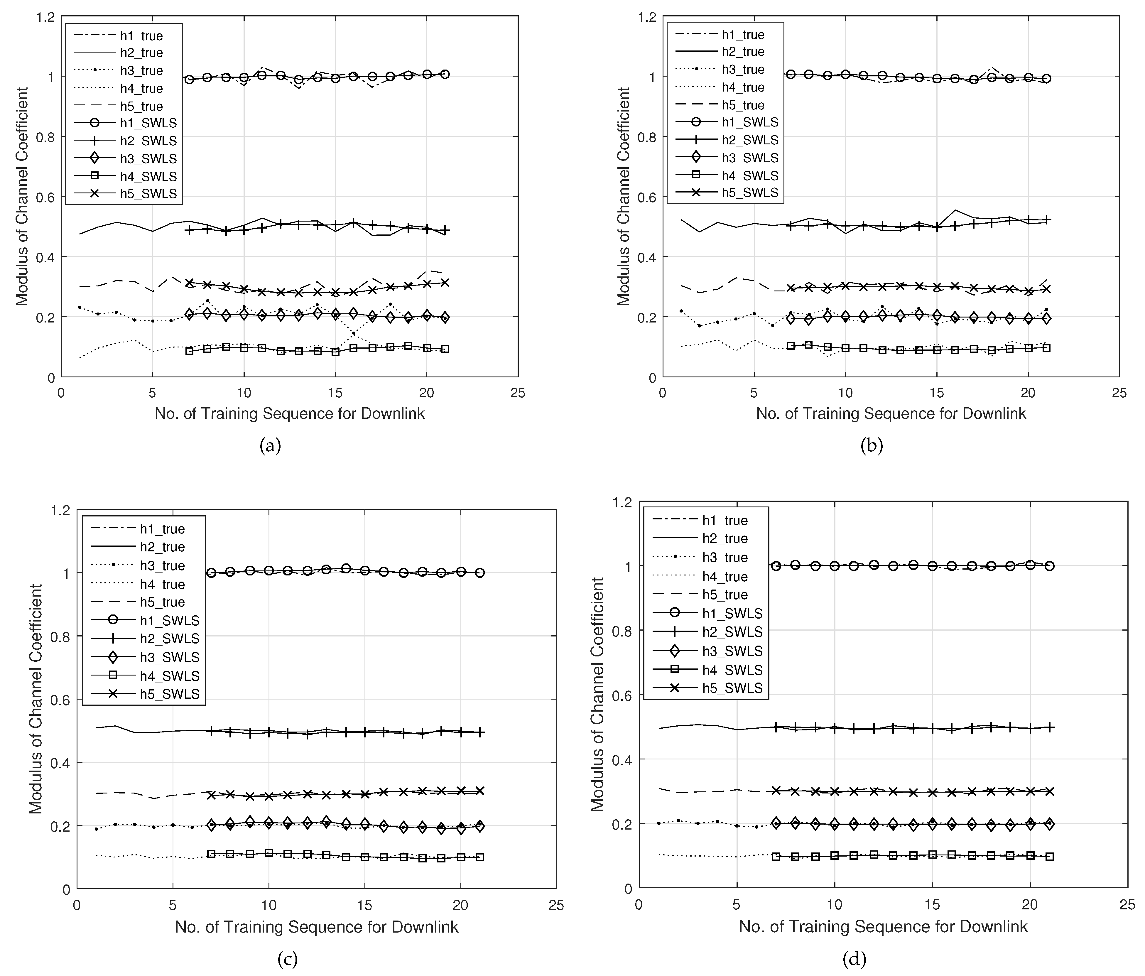
Figure 5 demonstrates the tracking performance of CTA_SWLS according to the MSE. Different noise levels only affected the mean value of the deviation, as shown by, for example, the fixed distance between the two curves at the top and bottom of Figure 5a,b, which was consistent with III in (38). However, the magnitude of the deviation was only affected by the channel jitter, which agreed with I and II in (38). In addition, the curves exhibited a cyclic pattern of the downlink with respect to the number of training sequences due to the cyclical sending of P sequences, which was in agreement with II of (38). Therefore, the theoretical variance of CTA_SWLS given by (38) was confirmed through this simulation.

5.2. IQI and PA Nonlinearity Estimation Performance via IQINSEA in Case A and Case B

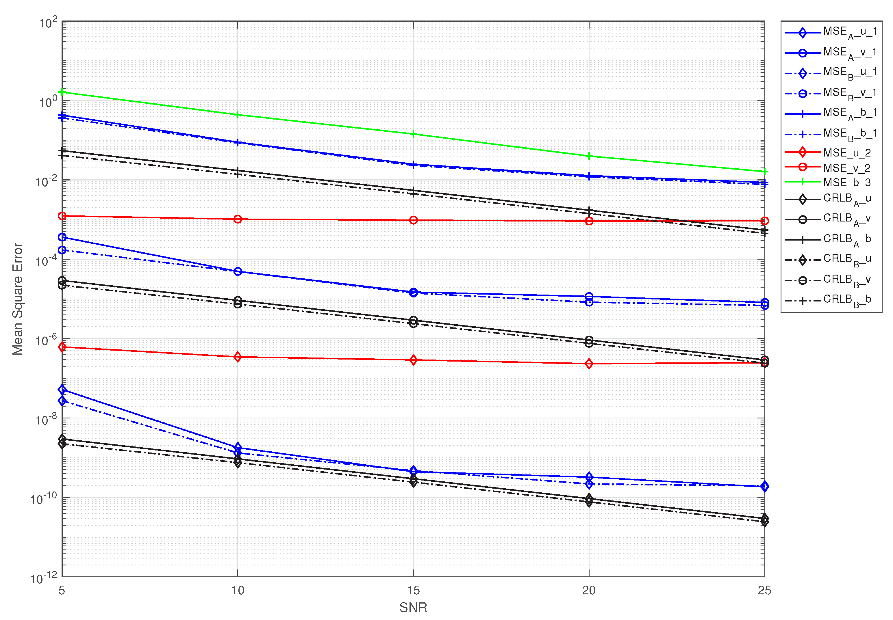
Figure 6, Figure 7 and Figure 8 show the MSE performance curves versus the SNR for IQINSEA in the two cases. The IQI and PA nonlinearity parameters were configured as follows: strong IQI and strong PA nonlinearity in Figure 6, strong IQI and weak PA nonlinearity in Figure 7, and weak IQI and strong PA nonlinearity in Figure 8. It was considered that the proposed scheme had to estimate the CSI first for both cases before the IQI and PA nonlinearity could be estimated by using IQINSEA. To facilitate fair comparisons, the ideal CSI was provided for method 2 and method 3; otherwise, the estimation performance of these two algorithms would be worse. Under this condition, since method 2 did not have the ability to estimate the PA nonlinearity and method 3 could not estimate the IQI, method 2 was only involved in the estimation of the IQI, and method 3 was only involved in the estimation of the PA nonlinearity.

In Figure 6, it can be observed that, in the strong IQI scenarios, the PA nonlinearity estimation with method 3 hardly improved as the SNR grew (Figure 6 and Figure 7) because this method did not take the IQI into account, although there was some improvement in the weak IQI scenario (Figure 8). Accordingly, it can be seen that the effect of the IQI on the estimation performance of method 3 was relatively large. Note that the MSE performance of method 2 hardly varied with the SNR in all of the scenarios because this method is prone to local minima and does not consider the PA nonlinearity. These results were obtained with the assumption that the CSI was known at the BS for methods 2 and 3. Otherwise, the estimated errors would be even larger.

Nevertheless, of all of the scenarios, our proposed scheme was the most efficient among the three methods, i.e., it had a lower MSE and was closer to the CRLB. Another noteworthy aspect is that the MSE curves slowly decreased as the SNR grew, especially in the high-SNR regime. Note that the MSEs in case B were slightly lower than those in case A, especially with a low SNR, which verified the conclusion given in Section 4. This is because when the CSI was estimated, it was placed at the transmitter to directly remove the effect of the CSI on the system; then, the signal without the impact of the CSI was transmitted, i.e., case B. On the contrary, the CSI was further distorted in transmission, resulting in the removal of the impact of the CSI on the system at the receiver, thus making the error of the system larger, i.e., case A.

6. Conclusions

In this study, two important features of a transmitter, i.e., IQI and PA nonlinearity, were utilized, and these are generated by the nonlinear circuit of the RF front-end at the terminal. They are detrimental to the efficiency of data transmission, but due to their uniqueness and long-term invariance, they can be used as RF fingerprints of a transmitter for terminal identification. This study focuses on the problem of extracting the IQI and PA nonlinearity of a transmitter efficiently and separately in the presence of multiple paths for TDD OFDM systems.

Via system modeling, it was found that only a single transmission could not yield a unique solution due to the coexistence of the IQI, PA nonlinearity, and multiple paths. To address this intractable problem, we proposed a scheme for independently estimating the IQI and nonlinearity, and this involved two round trips with four steps.

Once the training sequences from the BS were received, the real-time CSI was first estimated/tracked at the terminal by using the CTA_SWLS algorithm. The procedures were then divided into different parts for the two cases. In case A, the IQI and PA nonlinearity were unknown at the terminal; in case B, the IQI and PA nonlinearity were known at the terminal. In the two cases, the treatments for removing the impact of the CSI were distinct. Finally, the IQI and PA nonlinearity were estimated at the receiver by using IQINSEA.

With the theoretical analysis, the CSI tracking performance of CTA_SWLS was given. The influence of error propagation on further processing stages was given for both cases. Then, the approximate unbiasedness of the estimation algorithm was theoretically proven, and the variances of IQINSEA were given with the CRLB for both cases. The numerical results show the efficiency of the scheme in comparison with existing techniques in the literature.