AI-Enabled Framework for Mobile Network Experimentation Leveraging ChatGPT: Case Study of Channel Capacity Calculation for η-µ Fading and Co-Channel Interference

Abstract

Artificial intelligence has been identified as one of the main driving forces of innovation in state-of-the-art mobile and wireless networks. It has enabled many novel usage scenarios, relying on predictive models for increasing network management efficiency. However, its adoption requires additional efforts, such as mastering the terminology, tools, and newly required steps of data importing and preparation, all of which increase the time required for experimentation. Therefore, we aimed to automate the manual steps as much as possible while reducing the overall cognitive load. In this paper, we explore the potential use of a novel Chat Generative Pre-trained Transformer (ChatGPT) conversational agent together with a model-driven approach relying on the Neo4j graph database in order to aid experimentation and analytics in the case of wireless network planning. As a case study, we present a derivation of the expression for the channel capacity (CC) metric in the case of η-µ multipath fading and η-µ co-channel interference. Moreover, the derived expression is leveraged for quality of service (QoS) estimation within the software simulation environment. ChatGPT, in synergy with a model-driven approach, is used to automate several steps: data importing, generation of graph construction, and machine learning-related Neo4j queries. According to the achieved outcomes, the proposed QoS estimation method, based on the derived CC expression (with precision up to the fifth significant digit), demonstrates satisfactory accuracy (up to 98%) and faster training than the deep neural network-based solution. On the other hand, compared to the manual approach based on our previous work, ChatGPT-based code generation reduces the time required for experimentation by more than 4 times.

1. Introduction

Propagation in mobile radio environments is characterized by waves that interact with the surfaces of the objects they encounter. These waves react through phenomena such as diffraction, reflection, refraction, scattering, and absorption, causing the signal to fade rapidly. This is referred to as short-term fading [1].

The amplitudes and phases of the propagation waves vary in accordance with the physical properties of the surfaces they encounter. Various distributions can describe these variations. Among them is the η-µ distribution [2] and the so-called η-µ fading, which influences mobile networks. The η-µ fading model observes a signal consisting of clusters of multipath waves that propagate in an inhomogeneous environment. Within any cluster, the phases of the scattered waves are random and have similar delay times, but there is a relatively large spread in the delay times of different clusters [2]. The η-µ distribution is a general fading distribution used to faithfully represent the small-scale variation of the fading signal, provided there is no line-of-sight [3].

Because of its generality, the impact of this fading on wireless systems has been extensively discussed in the literature. Various aspects of wireless systems’ performance under the influence of fading effects have been evaluated for different purposes. In [4,5,6,7,8], the first-order system performance in the presence of η-µ fading was derived. In [4], the moment generating function (MGF) of the generalized η-µ distribution was derived and used to evaluate the average bit error rate (ABER) in η-µ fading channels in terms of elementary functions. An exact closed-form expression for the outage probability (OP) in η-µ fading channels was derived in [5]. Reference [6] investigated the ABER and OP of binary coherent, and non-coherent modulation schemes were obtained for an L-branch maximal ratio combining (MRC) diversity receiver over exponentially correlated η-µ fading channels. In [7], expressions for the rate and OP were developed for the MRC receiver in scenarios involving η-µ fading and interferers with unequal power. Reference [8] provided exact closed-form expressions for the OP of MRC in η-µ fading channels with antenna correlation and Rayleigh co-channel interference (CCI) with arbitrary powers.

The second-order performance of wireless systems in the presence of η-µ fading was considered in [9,10]. The formula for the level crossing rate (LCR) was derived in [9] for the selection combining (SC) receiver in mobile systems under the influence of η-µ fading and η-µ CCI. The LCR, the average fade duration (AFD), and the phase crossing rate (PCR) were derived in [10] for η-µ fading channels.

The channel capacity (CC) is one of the most important performance metrics of the first order. Increasing the CC of mobile networks is one of the main demands in today’s wireless services. Analyses of the channel capacity can be found in the existing literature [11,12,13]. This is why we have chosen to investigate this performance metric in our paper.

In addition to small-scale fading, CCI is also present in wireless systems. It can be a consequence of different influences, including the weather conditions, administrative factors, or design issues. References [8,9,10] took into account the impact of CCI, in addition to the η-µ fading. CCI can also be modeled with different distributions.

The standard approach to mitigating the impact of fading and CCI is through diversity combining [1]. Some of the most common diversity-combining techniques are maximal ratio combining (MRC) [6,7,8], equal gain combining (EGC) [14], and selection combining (SC) [9,13,15]. While all of these techniques improve system performance, MRC is considered the most effective. On the other hand, SC combining has a lower cost and still good enough features for mitigating fading and CCI. Therefore, in this paper, we analyze a multi-branch SC receiver used to enhance wireless systems in the presence of η-µ fading and CCI. Since this scenario has an important vehicular application, we derive its CC expression.

On another front, artificial intelligence (AI) has opened new horizons for wireless network planning, especially in proactive performance-related infrastructure reconfiguration and tuning [16]. Realistic environments also encompass negative effects on propagated waves, which must be considered in these predictions. However, the rise of AI-based tools and rapid advancements in this area have made simulation workflows increasingly complex, demanding a higher cognitive load to master the related concepts and techniques. As a downside, because adopting novel techniques requires additional effort, the time required for insightful network planning has increased, consequently slowing down prototyping and research. Hence, in this paper, we focus on providing an automated network simulation workflow that integrates AI tools to reduce the time needed for simulation. The presented case study considers environments influenced by η-µ multipath fading and η-µ co-channel interference. To the best of our knowledge, there is no other publicly available scientific work that adopts Chat Generative Pre-trained Transformer (ChatGPT) in combination with a model-driven approach for the purpose of graph database-related code generation in the field of telecommunications.

The main contributions of this paper are as follows:

(1)

We derive the expression for CC for the L-branch SC receiver in the case of η-µ multipath fading and η-µ CCI;

(2)

We present a QoS estimation model based on classifications within the Neo4j graph database, leveraging the previously derived CC as one of the inputs;

(3)

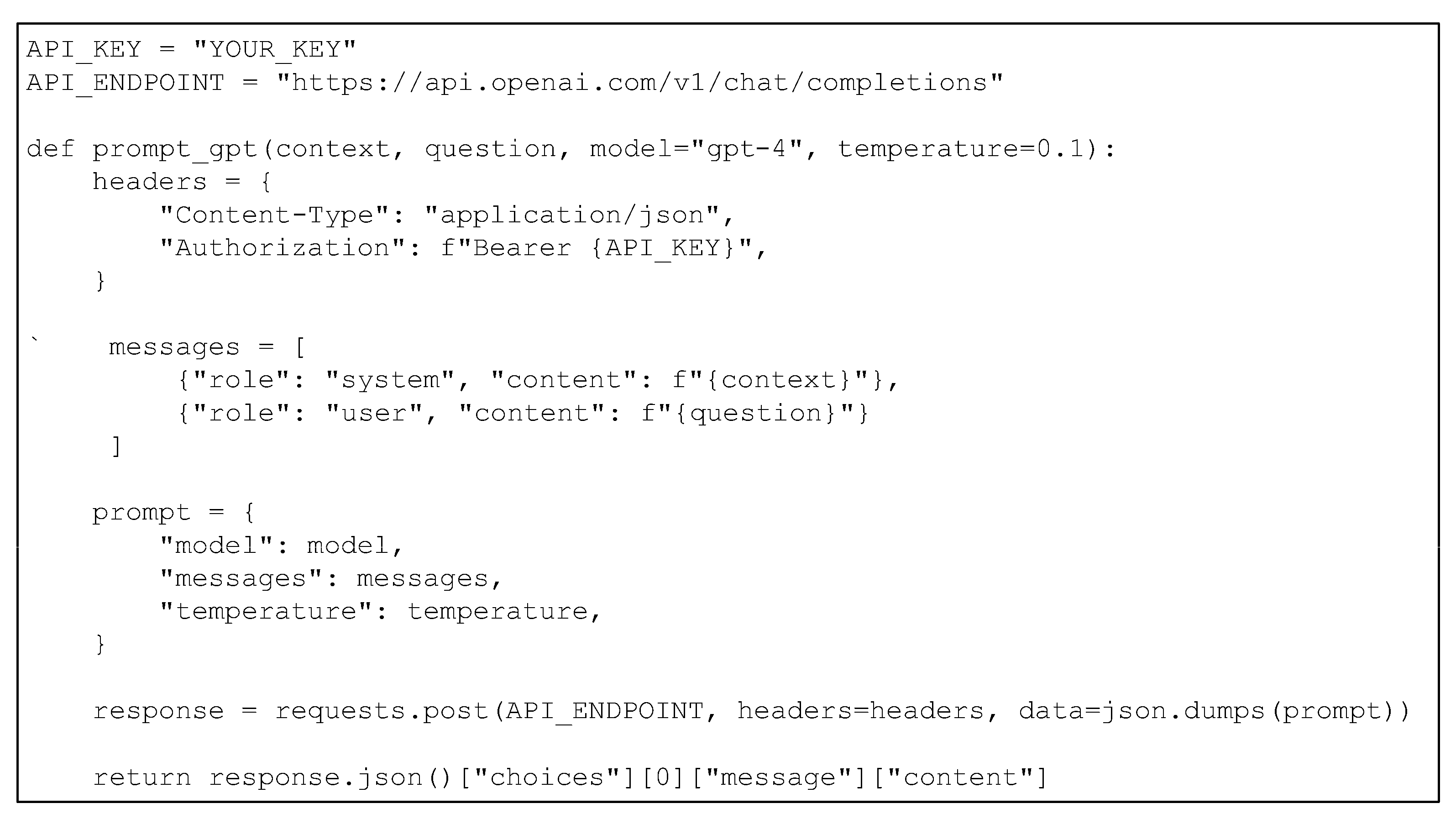
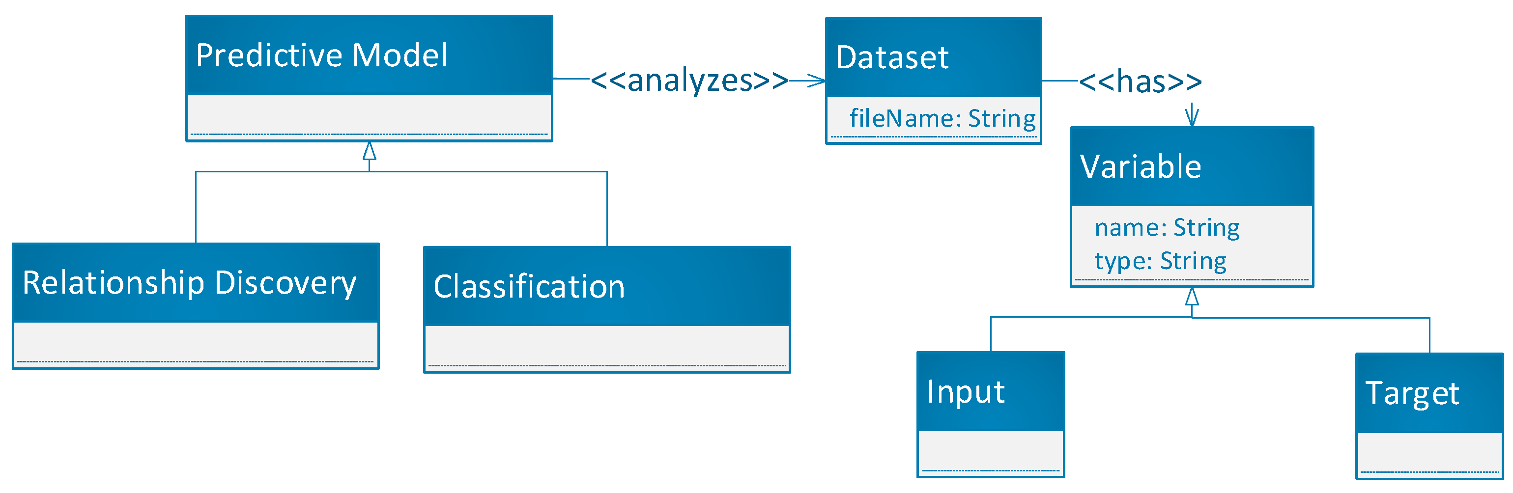
We propose a ChatGPT-based approach to automated Neo4j query generation, covering data import and classification using a meta-model.

This paper is organized into four main sections and includes two appendices. Following Section 1, we derive the CC expression, and analyze the influence of the parameters based on the results in plotted graphs. Afterwards, we propose a classification-based method for quality of service (QoS) prediction, utilizing the previously derived CC expression within the network planning environment to calculate one of the input variables. In this section, we also provide an overview of the underlying framework for machine learning capabilities—the Neo4j graph database and its graph data science (GDS) library. Additionally, we give background information about large language models (LLMs) and model-driven engineering, as they represent the underlying concepts behind ChatGPT and Ecore. The synergy of these two is leveraged with the aim of automatizing a machine learning-aided simulation workflow for mobile network planning. While Ecore-based models were used for prompt construction, we relied on ChatGPT for Neo4j query generation based on these prompts. At the end of the third section, we evaluate the benefits of the proposed approach and provide a comparison to the manual procedure. Finally, the achieved QoS estimation performance is compared to other similar work. The fourth section summarizes the results and discusses possible future research directions. The appendices offer additional details on the derivation of the CC expression and the intermediate steps.

2. Channel Capacity in the Presence of η-µ Fading and CCI

2.1. Derivation of the PDF of the Receiver’s Output Signal-to-Co-Channel Interference Ratio

In this section, we derive the probability density function (PDF) of the output signal-to-co-channel interference-ratio (SIR) for a multi-branch SC receiver within a wireless system disturbed by η-µ fading and η-µ distributed CCI. The use of appropriate fading and CCI models is valuable for addressing challenges related to channel capacity maximization within wireless systems.

From the very name of the distribution, we can deduce that the η-µ distribution is characterized by two parameters. The parameter η represents the ratio of the powers of the in-phase and in-quadrature scattered waves in each multipath cluster, while µ denotes the number of clusters [2]. This distribution is derived from field measurements and is thus fully characterized in terms of measurable physical parameters [3].

The η-µ fading may appear in two different formats corresponding to two physical models. However, mathematically, one format can be obtained from the other using the following relation:

$${\mathsf{\eta }}_{\mathrm{Format}2}=\frac{1-{\mathsf{\eta }}_{\mathrm{Format}1}}{1+{\mathsf{\eta }}_{\mathrm{Format}1}} \mathrm{or} {\mathsf{\eta }}_{\mathrm{Format}1}=\frac{1-{\mathsf{\eta }}_{\mathrm{Format}2}}{1+{\mathsf{\eta }}_{\mathrm{Format}2}} ,$$

where 0 < η_Format1 < ∞ is the η parameter in Format 1, and −1 < η_Format2 < 1 is the η parameter in Format 2 [3].

To simplify the notation, η is used in both cases, keeping in mind that they represent different physical phenomena, and that their domains are different. Further simplification is achieved by defining two new parameters, denoted h and H and both functions of η. These parameters hold distinct meanings and values for the two different formats. The convenience of using h and H is that they have a unique representation for both formats [3].

In Format 1, we have h = (2 + η⁻¹ + η)/4 and H = (η⁻¹ − η). When 0 < η $\le$ 1, then H $\ge$ 0, while for 0 < η⁻¹ $\le$ 1, we have H $\le$ 0. It is important to note that due to the property I_ν(−z) = (−1)^v I_ν(z), the distribution yields identical values within these two intervals, i.e., it is symmetrical around η = 1. Therefore, it is sufficient to consider η within one of these ranges. Also, in Format 1, we observe that H/h = (1 − η)/ (1 + η) [3].

The Hoyt (Nakagami-q), one-sided Gaussian, Nakagami-m, and Rayleigh distributions are all special cases of the η-µ distribution. The Hoyt (or Nakagami-q) distribution is obtained by setting µ = 0.5, the one-sided Gaussian distribution emerges as η approaches 0 or ∞, whereas the Rayleigh distribution corresponds exactly to µ = 0.5 and η = 1.

If L denotes the number of input branches in the multi-branch SC receiver, under the η-µ distribution, the signal envelopes at the receiver inputs x_i, i = 1, 2, …, L, are ([9]; (3)):

$$p_{x_i}\left(x_i\right)=\frac{4\sqrt{\pi } h_1{}^{{\mu }_1}}{\mathsf{\Gamma }\left({\mu }_1\right){\mathrm{e}}^{\frac{2{\mu }_1{h}_1}{{\mathsf{\Omega }}_i}{x}_i{}^2}}{\displaystyle \sum _{i_1=0}^{+\infty }\frac{H_1{}^{2i_1}{x}_i{}^{4i_1+4{\mu }_1-1}{\left({\mu }_1/{\mathsf{\Omega }}_i\right)}^{2i_1+2{\mu }_1}}{i_1!\mathsf{\Gamma }\left(i_1+{\mu }_1+1/2\right)}}.$$

(1)

Ω_i represents the mean values of the input signals: Ω_i =${\overline{x}}_i^2$ and Γ(·) is the Gamma function ([17]; Sec. (8.31)).

Since the η-µ distribution is of Format 1 [3], its parameters are defined as:

$$h_1=\frac{2+{\mathsf{\eta }}_1{}^{-1}+{\mathsf{\eta }}_1}{4}, H_1=\frac{{\mathsf{\eta }}_1{}^{-1}-{\mathsf{\eta }}_1}{4}.$$

(2)

Applying Expression (2) to Expression (1), we obtained the PDF of the input signal to the SC combiner in the following form:

$$p_{x_i}\left(x_i\right)=\frac{4\sqrt{\pi } {\left({\mathsf{\eta }}_1+1\right)}^{2{\mu }_1}}{\mathsf{\Gamma }\left({\mu }_1\right){\mathrm{e}}^{\frac{{\mu }_1{\left({\mathsf{\eta }}_1+1\right)}^2}{2{\mathsf{\eta }}_1{\mathsf{\Omega }}_i}{x}_i{}^2}}{\displaystyle \sum _{i_1=0}^{+\infty }\frac{{\left(1-{\mathsf{\eta }}_1{}^2\right)}^{2i_1}{x}_i{}^{4i_1+4{\mu }_1-1}{\left({\mu }_1/{\mathsf{\Omega }}_i\right)}^{2i_1+2{\mu }_1}}{2^{4i_1+2{\mu }_1}{\mathsf{\eta }}_1{}^{2i_1+{\mu }_1}\mathsf{\Gamma }\left(i_1+{\mu }_1+1/2\right)i_1!}}.$$

(3)

In the observed environment, the input CCI envelopes, marked with y_i, i = 1, 2, ..., L, also follow the η-µ distribution:

$$p_{y_i}\left(y_i\right)=\frac{4\sqrt{\pi } {\left({\mathsf{\eta }}_2+1\right)}^{2{\mu }_2}}{\mathsf{\Gamma }\left({\mu }_2\right){\mathrm{e}}^{\frac{{\mu }_2{\left({\mathsf{\eta }}_2+1\right)}^2}{2{\mathsf{\eta }}_2{s}_i}{y}_i{}^2}}{\displaystyle \sum _{i_2=0}^{+\infty }\frac{{\left(1-{\mathsf{\eta }}_2{}^2\right)}^{2i_2}{y}_i{}^{4i_2+4{\mu }_2-1}{\left({\mu }_2/s_i\right)}^{2i_2+2{\mu }_2}}{2^{4i_2+2{\mu }_2}{\mathsf{\eta }}_2{}^{2i_2+{\mu }_2}\mathsf{\Gamma }\left(i_2+{\mu }_2+1/2\right)i_2!}}.$$

(4)

The mean square values of the CCI envelopes are denoted by s_i, s_i = ${\overline{y}}_i^2$, i = 1, 2, ..., L.

The ratio of the desired signal envelope and the CCI envelope at the ith input branch of the SC receiver is denoted by z_i, z_i = x_i/y_i, and has the following PDF [18]:

$$p_{z_i}\left(z_i\right)={\displaystyle \underset{0}{\overset{\infty }{\int }}{y}_i{p}_{x_i}}\left(z_i{y}_i\right)p_{y_i}\left(y_i\right)d{y}_i.$$

(5)

After introducing Equations (3) and (4) into (5), we have the PDF of the SIR z_i:

$$\begin{gathered} p_{z_i}\left(z_i\right)=\frac{8\pi {\left({\mathsf{\eta }}_1+1\right)}^{2{\mu }_1} {\left({\mathsf{\eta }}_2+1\right)}^{2{\mu }_2}}{\mathsf{\Gamma }\left({\mu }_1\right)\mathsf{\Gamma }\left({\mu }_2\right)}{\displaystyle \sum _{i_1=0}^{+\infty }{\displaystyle \sum _{i_2=0}^{+\infty }\frac{{\left(1-{\mathsf{\eta }}_1{}^2\right)}^{2i_1}{\left(1-{\mathsf{\eta }}_2{}^2\right)}^{2i_2}{\mu }_1{}^{2i_1+2{\mu }_1}{\mu }_2{}^{2i_2+2{\mu }_2}}{2^{2i_1+2i_2}{i}_1!i_2!\mathsf{\Gamma }\left(i_1+{\mu }_1+1/2\right)}}}\times \\ \frac{{\mathsf{\eta }}_1{}^{2i_2+{\mu }_1+2{\mu }_2}{\mathsf{\eta }}_2{}^{2i_1+2{\mu }_1+{\mu }_2}\mathsf{\Gamma }\left(2i_1+2i_2+2{\mu }_1+2{\mu }_2\right){\mathsf{\Omega }}_i{}^{2i_2+2{\mu }_2}{s}_i{}^{2i_1+2{\mu }_1}{z}_i{}^{4i_1+4{\mu }_1-1}}{\mathsf{\Gamma }\left(i_2+{\mu }_2+1/2\right){\left({\mathsf{\eta }}_1{\mu }_2{\mathsf{\Omega }}_i{\left({\mathsf{\eta }}_2+1\right)}^2+{\mathsf{\eta }}_2{\mu }_1{s}_i{\left({\mathsf{\eta }}_1+1\right)}^2{z}_i{}^2\right)}^{2i_1+2i_2+2{\mu }_1+2{\mu }_2}} \end{gathered}$$

(6)

The cumulative distribution function (CDF) of SIRs z_i is derived in Appendix A and is given by Formula (A5):

$$\begin{gathered} F_{z_i}\left(z_i\right)=\frac{4\pi {\mathsf{\eta }}_1{}^{{\mu }_1} }{\mathsf{\Gamma }\left({\mu }_1\right)\mathsf{\Gamma }\left({\mu }_2\right)}{\displaystyle \sum _{i_1=0}^{+\infty }{\displaystyle \sum _{i_2=0}^{+\infty }{\displaystyle \sum _{i_3=0}^{+\infty }\frac{{\left(2i_1+2{\mu }_1\right)}_{i_3}{\left(1-2i_2-2{\mu }_2\right)}_{i_3}{\left({\mathsf{\eta }}_1+1\right)}^{2i_3+2{\mu }_1}{\left(1-{\mathsf{\eta }}_1{}^2\right)}^{2i_1}{\left(1-{\mathsf{\eta }}_2{}^2\right)}^{2i_2}}{2^{2i_1+2i_2}{\left(2i_1+2{\mu }_1+1\right)}_{i_3}{\left({\mathsf{\eta }}_2+1\right)}^{4i_2+2{\mu }_2}{i}_1!i_2!i_3!}}}}\times \\ \frac{\mathsf{\Gamma }\left(2i_1+2i_2+2{\mu }_1+2{\mu }_2\right){\mathsf{\eta }}_2{}^{2i_1+i_3+2{\mu }_1+{\mu }_2}}{\mathsf{\Gamma }\left(i_1+{\mu }_1+1/2\right)\mathsf{\Gamma }\left(i_2+{\mu }_2+1/2\right)\left(2i_1+2{\mu }_1\right)}{\left(\frac{{\mu }_1{s}_i{z}_i{}^2}{{\mathsf{\eta }}_1{\mu }_2{\mathsf{\Omega }}_i{\left({\mathsf{\eta }}_2+1\right)}^2+{\mathsf{\eta }}_2{\mu }_1{s}_i{\left({\mathsf{\eta }}_1+1\right)}^2{z}_i{}^2}\right)}^{2i_1+i_3+2{\mu }_1}. \end{gathered}$$

(7)

Now, Equation (7) gives the CDF for the SIR from each input branch.

After passing the signal through the SC receiver, it chooses the branch with the highest SIR from all input antennas based on the SC combiner, with the L branches operation algorithm. The signal from that selected input branch is then fed to the user. The output SIR is denoted as z and defined by z = max(z₁, z₂, …, z_L), where i = 1, 2, …, L. The PDF of the SIR z at the output of the multi-branch SC receiver will be calculated based on the expression ([15], (4)):

$$p_z\left(z\right)=L{p}_{z_i}\left(z_i\right){\left(F_{z_i}\left(z_i\right)\right)}^{L-1}.$$

(8)

By substituting Equations (6) and (7) into Equation (8), the PDF of the output SIR z is:

$$\begin{gathered} p_z\left(z\right)=\frac{2L }{{\left({\mathsf{\eta }}_2+1\right)}^{2L{\mu }_2-4{\mu }_2}} {\left(\frac{4\pi {\left({\mathsf{\eta }}_1+1\right)}^{2{\mu }_1}}{\mathsf{\Gamma }\left({\mu }_1\right)\mathsf{\Gamma }\left({\mu }_2\right)}\right)}^L{\displaystyle \sum _{i_1=0}^{+\infty }{\displaystyle \sum _{i_2=0}^{+\infty }\frac{{\left(1-{\mathsf{\eta }}_1{}^2\right)}^{2i_1}{\left(1-{\mathsf{\eta }}_2{}^2\right)}^{2i_2}{\mathsf{\eta }}_1{}^{2i_2+L{\mu }_1+2{\mu }_2} }{2^{2i_1+2i_2}\mathsf{\Gamma }\left(i_1+{\mu }_1+1/2\right)}\times }} \\ \frac{{\mathsf{\eta }}_2{}^{2i_1+2L{\mu }_1+L{\mu }_2}\mathsf{\Gamma }\left(2i_1+2i_2+2{\mu }_1+2{\mu }_2\right){\left({\mu }_1{s}_i\right)}^{2i_1+2L{\mu }_1}{\left({\mu }_2{\mathsf{\Omega }}_i\right)}^{2i_2+2{\mu }_2}{z}_i{}^{4i_1+4L{\mu }_1-1}}{\mathsf{\Gamma }\left(i_2+{\mu }_2+1/2\right){\left({\mathsf{\eta }}_1{\mu }_2{\mathsf{\Omega }}_i{\left({\mathsf{\eta }}_2+1\right)}^2+{\mathsf{\eta }}_2{\mu }_1{s}_i{\left({\mathsf{\eta }}_1+1\right)}^2{z}_i{}^2\right)}^{2i_1+2i_2+2L{\mu }_1+2{\mu }_2}{i}_1!i_2!}\times \\ \left({\displaystyle \sum _{i_3=0}^{+\infty }{\displaystyle \sum _{i_4=0}^{+\infty }{\displaystyle \sum _{i_5=0}^{+\infty }\frac{{\left(2i_3+2{\mu }_1\right)}_{i_5}{\left(1-2i_4-2{\mu }_2\right)}_{i_5}{\left({\mu }_1{s}_i{\mathsf{\eta }}_2{z}_i{}^2\right)}^{2i_3+i_5}{\left({\mathsf{\eta }}_1+1\right)}^{2i_5}{\left(1-{\mathsf{\eta }}_1{}^2\right)}^{2i_3}}{2^{2i_3+2i_4}{\left(2i_3+2{\mu }_1+1\right)}_{i_5}\mathsf{\Gamma }\left(i_3+{\mu }_1+1/2\right){\left({\mathsf{\eta }}_2+1\right)}^{4i_4}\mathsf{\Gamma }\left(i_4+{\mu }_2+1/2\right)}}}}\right.\times \\ {\left.\frac{{\left(1-{\mathsf{\eta }}_2{}^2\right)}^{2i_4}\mathsf{\Gamma }\left(2i_3+2i_4+2{\mu }_1+2{\mu }_2\right)}{i_3!i_4!i_5!\left(2i_3+2{\mu }_1\right){\left({\mathsf{\eta }}_1{\mu }_2{\mathsf{\Omega }}_i{\left({\mathsf{\eta }}_2+1\right)}^2+{\mathsf{\eta }}_2{\mu }_1{s}_i{\left({\mathsf{\eta }}_1+1\right)}^2{z}_i{}^2\right)}^{2i_3+i_5}}\right)}^{L-1}. \end{gathered}$$

(9)

2.2. Channel Capacity Derivation

In this subsection, we derive the channel capacity for the multi-branch SC receiver in a wireless system disturbed by η-µ fading and η-µ distributed CCI. The channel capacity is a performance measure of utmost importance in wireless communication system design because it provides information about the upper bound of the maximal transmission rate. The average CC normalized by the bandwidth B, given in Hz, is obtained in ([1], (17.4))

$$\frac{CC}{B}=\frac{1}{\ln \left(2\right)}{\displaystyle \underset{0}{\overset{\infty }{\int }}\ln \left(1+z\right)}{p}_z\left(z\right)dz$$

(10)

where CC represents the Shannon capacity in bits/s.

Using mathematical manipulations done in Appendix B, we obtained the normalized CC in its final form in (A9):

$$\begin{gathered} \frac{CC}{B}=\frac{L}{\ln \left(2\right)}{\left(\frac{4\pi }{\mathsf{\Gamma }\left({\mu }_1\right)\mathsf{\Gamma }\left({\mu }_2\right)}\right)}^L\left({\displaystyle \sum _{i_1=0}^{+\infty }{\displaystyle \sum _{i_2=0}^{+\infty }{\displaystyle \sum _{i_3=0}^{+\infty }\frac{{\left(-1\right)}^{i_1} {\left(1-{\mathsf{\eta }}_1{}^2\right)}^{2i_2}{\left(1-{\mathsf{\eta }}_2{}^2\right)}^{2i_3} }{2^{2i_2+2i_3}{i}_2!i_3!\left(i_1+1\right)!{\mathsf{\eta }}_2{}^{\left(i_1-2L{\mu }_2+1\right)/2}}}}}\right.\times \\ \frac{{\mathsf{\eta }}_1{}^{\left(i_1+2L{\mu }_1+1\right)/2}\mathsf{\Gamma }\left(2i_2+2i_3+2{\mu }_1+2{\mu }_2\right){\left({\mu }_2{\mathsf{\Omega }}_i/{\mu }_1{s}_i\right)}^{\left(i_1+1\right)/2}}{\mathsf{\Gamma }\left(i_2+{\mu }_1+1/2\right)\mathsf{\Gamma }\left(i_3+{\mu }_2+1/2\right){\left({\mathsf{\eta }}_1+1\right)}^{i_1+4i_2+2L{\mu }_1+1}{\left({\mathsf{\eta }}_2+1\right)}^{4i_3+2L{\mu }_2-i_1-1}}\times \\ \left({\displaystyle \sum _{i_4=0}^{+\infty }{\displaystyle \sum _{i_5=0}^{+\infty }{\displaystyle \sum _{i_6=0}^{+\infty }\frac{{\left(2i_4+2{\mu }_1\right)}_{i_6}{\left(1-2i_5-2{\mu }_2\right)}_{i_6}}{2^{2i_4+2i_5}{\left(2i_4+2{\mu }_1+1\right)}_{i_6}{i}_4!i_5!i_6!\mathsf{\Gamma }\left(i_4+{\mu }_1+1/2\right)}}}}\right.\times \\ {\left.{\left(\frac{1-{\mathsf{\eta }}_1{}^2}{{\left({\mathsf{\eta }}_1+1\right)}^2}\right)}^{2i_4}{\left(\frac{1-{\mathsf{\eta }}_2{}^2}{{\left({\mathsf{\eta }}_2+1\right)}^2}\right)}^{2i_5}\frac{\mathsf{\Gamma }\left(2i_4+2i_5+2{\mu }_1+2{\mu }_2\right)}{\mathsf{\Gamma }\left(i_5+{\mu }_2+1/2\right)\left(2i_4+2{\mu }_1\right)}\right)}^{L-1}\times \\ \left.B\left(\frac{i_1+4i_2+\left(4i_4+2i_6\right)\left(L-1\right)+4L{\mu }_1+1}{2},\frac{4i_3+4{\mu }_2-i_1-1}{2}\right)\right). \end{gathered}$$

(11)

The normalized CC depends on the parameters of η-µ fading and CCI as a triple sum whose rapid convergence is shown in

Table 1. The number of additions in the summation of Expression (11) to achieve precision at the fifth significant digit for variable parameters µ₁ and µ₂.

Variables	w = −10 dB	w = 0 dB	w = 10 dB
µ1 = 1, µ2 = 1	15	17	17
µ1 = 1.5, µ2 = 1	16	17	18
µ1 = 2, µ2 = 1	18	19	20
µ1 = 2.5, µ2 = 1	19	19	20
µ1 = 3, µ2 = 1	19	21	22
µ1 = 4, µ2 = 1	22	22	24
µ1 = 1, µ2 = 1.5	15	17	18
µ1 = 1, µ2 = 2	17	18	19
µ1 = 1, µ2 = 2.5	18	19	20
µ1 = 1, µ2 = 3	19	20	21
µ1 = 1, µ2 = 4	21	22	22

and

Table 2. The number of additions in the summation of Expression (11) to achieve precision at the fifth significant digit for different values of parameters η₁ and η₂, and number of branches L.

Variables	w = −10 dB	w = 0 dB	w = 10 dB
η1 = 0.2, η2 = 0.2, L = 2	15	17	17
η1 = 0.4, η2 = 0.2, L = 2	14	14	15
η1 = 0.6, η2 = 0.2, L = 2	13	15	16
η1 = 0.8, η2 = 0.2, L = 2	14	14	15
η1 = 0.2, η2 = 0.4, L = 2	15	16	16
η1 = 0.2, η2 = 0.6, L = 2	15	15	16
η1 = 0.2, η2 = 0.8, L = 2	15	16	15
η1 = 0.2, η2 = 0.2, L = 3	15	16	18
η1 = 0.2, η2 = 0.2, L = 4	17	17	17
η1 = 0.2, η2 = 0.2, L = 5	16	18	18

. In the next subsection, based on the calculation from Equation (11), we present the graphical analysis of the normalized CC of the wireless system in the presence of η-µ fading and CCI with the multi-branch SC receiver, along with the analysis of the parameters’ influence.

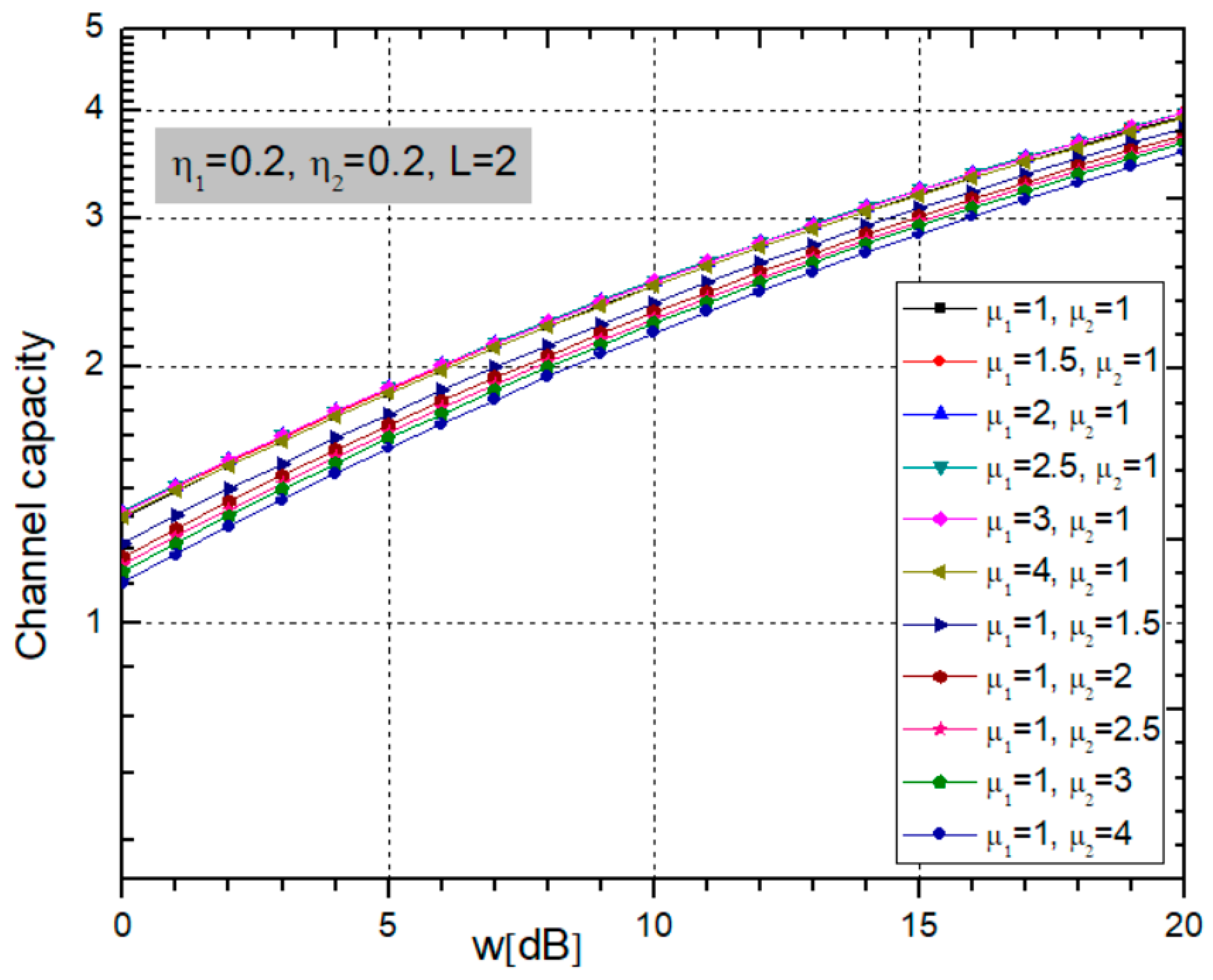
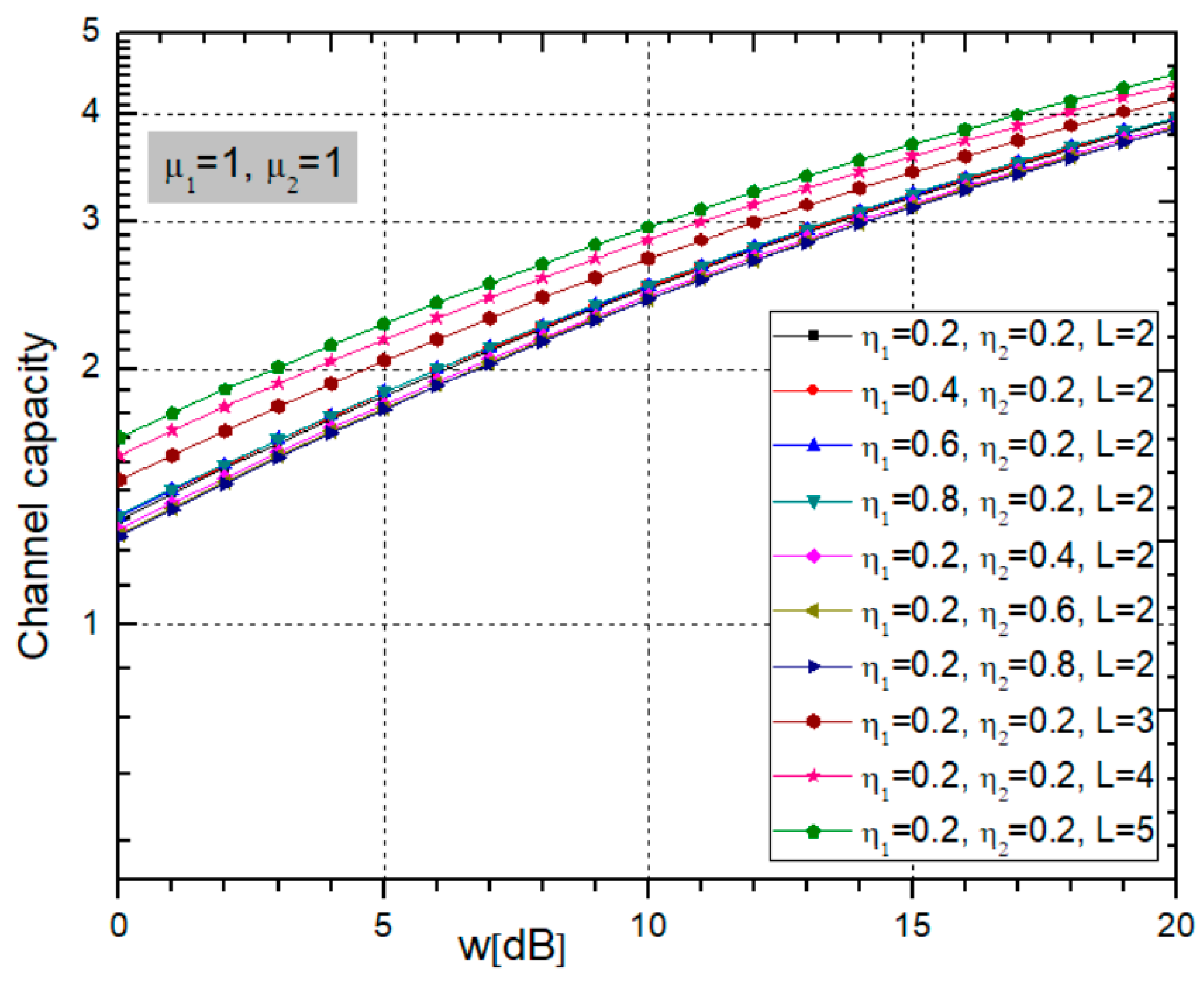
2.3. Analysis of Parameters’ Influence on the Channel Capacity

In order to analyze the impact of fading and CCI parameters on the channel capacity, we plotted two figures of normalized CC versus the output ratio of the signal’s and CCI’s powers, denoted as w = Ω/s. We assumed that the correlation between the input branches in the SC receiver can be neglected. For graphical presentation, we used the programs Mathematica and Origin.

In Figure 1, the normalized CC is presented for different values of fading and CCI parameters µ₁ and µ₂. In this case, we supposed equal values of parameters η₁ and η₂: η₁ = η₂ = 0.2, and that there were two input branches going into the SC receiver. In this figure, it is possible to notice that changing µ₁ parameter had an insignificant impact on the CC, while an increase in the µ₂ parameter led to a decrease in the CC, indicating worse system performance.

On the other hand, in Figure 2, the normalized CC is shown for some values of the fading and CCI parameters η₁ and η₂, while keeping the parameters µ₁ and µ₂ constant: µ₁ = µ₂ = 1. In Figure 2, it is visible that changes in the values of the parameters η₁ and η₂ had no major influence on the CC. In contrast, with an increase in the number of input branches (denoted by L), the CC increased, indicating an improvement of the system’s performance.

Additionally, we provide two tables to illustrate the number of additions required to achieve the desired precision in the summation of Formula (11) for channel capacity, specifically, with accuracy up to the fifth decimal place.

Table 1 demonstrates how this number of additions changed when varying the parameters µ₁ and µ₂. As µ₁ and µ₂ increased, the number of elements to be added also increased, indicating that the series converged more slowly for all values of the SIR w.

Table 2 illustrates the variations in the number of additions required when the parameters η₁ and η₂, as well as the number of input branches L, were altered. When the parameter η₁ increased, there was a decrease in the number of elements that needed to be added, indicating a faster convergence of the series. When the parameter η₂ increased, the number of elements to be added exhibited different behaviors for different values of SIR w. For w = −10 dB it was 15, for w = 0 dB it was between 14 and 16, and for w = 10 dB it further increased, and the series converged more slowly. Additionally, when L increased, the number of summing elements reached a maximum of 16 for w = −10 dB, and 18 for w = 0 dB and w = 10 dB. In this scenario, the convergence was the slowest.

3. Model-Driven Approach to QoS Estimation Using Neo4j Graph Database Aided by ChatGPT

In this section, the proposed simulation workflow aiding network planning based on machine learning techniques, considering the CC value from the previous part as input, is described. Here, we give an overview of the three main concepts behind the approach, together with corresponding technologies: classification within a graph database using Neo4j and GDS, generative LLMs adoption for code generation relying on ChatGPT, and model-driven engineering with an eclipse modeling framework (EMF) and Ecore. After that, we describe the crucial components for the implementation of the proposed workflow: a classification-based predictive model using GDS, an Ecore meta-model for prompt parameter specification, and a code generation method based on model-to-prompt transformation leveraging ChatGPT. Finally, the last subsection gives a comparison of the achieved results (both prediction performance and code generation time) with similar solutions.

3.1. Neo4j and Graph Data Science Library

Neo4j [19] is a database management system based on a graph data model. The underlying data representation model consists of the following main concepts: (1) node—an entity that corresponds to an object or event within some domain of interest considered, (2) link—a relationship that connects two node elements, and (3) property—a pair in the form of (key, value) describing the characteristics of interest of a node or link. Additionally, in order to perform data management or retrieval based on such representation in Neo4j, Cypher query language [20] is used for this purpose. Additionally, an add-on called the Graph Data Science Library [21] was also introduced as an optional plug-in in Neo4j, integrating a low-code interface to a set of machine learning-oriented functionalities against the data graph. The main focus of the available algorithms forming GDS is on two tasks: classification and relationship discovery.

Despite the limited set of machine learning techniques that are supported by Neo4j, their implementation has been shown to be faster in training and more effective (higher prediction accuracy) compared to deep learning and other more complex neural network-based approaches in the case of simpler numeric data-based predictions, without involving audiovisual signals [22]. Considering that many cases rely on numeric data only, while the execution speed is crucial for real-time scenarios, Neo4j’s GDS library represents a reasonable choice when it comes to the adoption of AI in the area of wireless networks.

In order to train a classification model in GDS, we make use of the gds.alpha.ml.nodeClassification.train [23] procedure for this purpose.

Table 3. Steps for classification-based QoS estimation using GDS in Neo4j.

Step	Neo4j Query	Input	Output
Import data	LOAD CSV WITH HEADERS FROM ‘file:///qos_predict.csv’ AS row WITH row WHERE row.QoS IS NOT NULL MERGE (q:QosPredict {CC: row.CC,...QoS : row.QoS});	CSV tabular data	Internal tabular data representation
Graph construct	CALL gds.graph.create.cypher( ‘QosPredictGraph’, ‘MATCH (q:QosPredict) WHERE q.QoS is NOT NULL RETURN id(s) as id, q.CC as CC, ... q.QoS as QoS’, ‘MATCH (s:QosPredict)-[link]->(e:QosPredict) RETURN ID(link) as link, ID(s) as source, ID(e) as target’ )	Internal tabular data representation	Neo4j data graph
Classifier training	CALL gds.alpha.ml.nodeClassification.train( ‘QoSPredictGraph’, { modelName: ‘qos_prediction’, featureProperties: [‘CC’, ‘BsId’, . . .’Season’], targetProperty: ‘QoS’, randomSeed: 5, holdoutFraction: 0.20, validationFolds: 10, metrics: [ ‘ACCURACY’], params: [ { penalty: 0.01, maxEpochs: 10, batchSize: 5}, . . . { penalty: 0.001} ] }) YIELD modelInfo RETURN {penalty: modelInfo.bestParameters.penalty} AS winningModel, modelInfo.metrics.ACCURACY.outerTrain AS trainGraphScore, modelInfo.metrics.ACCURACY.test AS testGraphScore	Neo4j data graph	Predictive classification model

provides an overview of the queries used within the steps of the classification model creation. In this study, these queries were generated automatically using ChatGPT, starting from the model-based representation of a problem. The examples of queries are given in the case of a dataset for our QoS prediction case study.

3.2. ChatGPT and Large Language Models

ChatGPT [24] is a conversational agent service based on a large language model (LLM) for text generation, providing the ability to handle conversation in the form of dialogue. During the process of conversation, the user provides input in the form of a question, together with optional context containing additional facts that can be taken into account by ChatGPT in order to generate a more specific answer. It was publicly released by the OpenAI organization towards the end of 2022. Shortly after that, it started to draw large audience and public attention because of its comprehensiveness, thanks to the enormous amount of data used for the training of the underlying GPT model, which captured the state of the World Wide Web in textual form until late 2021. From poetry and essay writing, data analysis, code generation, and debugging to playing board games [24], ChatGPT has impressed its users around the world with its comprehensive and quite accurate answers. When it comes to the process of training, a customized transfer learning-alike approach was used, utilizing both supervised and reinforcement learning technique elements.

While ChatGPT can be accessed and used for free via an interactive web graphical user interface (GUI), it can be also accessed programmatically using a library that is available in all commonly used programming languages nowadays (such as Python or JavaScript). However, access to the application programming interface (API) requires an access OpenAPI token, while the programmatic requests themselves are charged based on a per-token pricing model (up to $0.02 per 1000 request tokens, which corresponds to roughly 750 words in length for the prompt and request). The latest version is currently GPT-4. However, there is still a limitation for the length of user-provided input/question, which is currently 3000 words. Regarding the programming paradigm for leveraging ChatGPT and similar LLMs, an approach known as prompt engineering or in-context learning is utilized [25]. During this process, model parameters are not modified, but rather, a mesa-optimization alike method is used, providing the capability to learn “small” models, which leverage the data provided as context for making more accurate predictions. Therefore, a user or a client of the ChatGPT service usually provides a prompt that consists of two parts: (1) a question—the task that we ask ChatGPT to solve, and (2) a context—a “hint” that helps ChatGPT to generate a more precise answer.

Once the prompt is constructed (which was carried out by processing the Ecore model, in our case), it is sent via an API as a request to the ChatGPT online service.

For this purpose, we made use of a Python script, as shown in Figure 3, built upon our previous work in the area of blockchain smart contract generation [26]. Once generated, it is forwarded as the input of a Python script, whose excerpt is given in Figure 3. Apart from the question and the context, we can also provide two additional parameters as input: (1) the model—a version of the underlying LLM, and (2) the temperature—a generated response randomness factor that we kept as low as possible, taking into account that deterministic answers were desired for our case study.

3.3. Model-Driven Engineering and Ecore

Model-driven engineering (MDE) is an approach for system development that considers models as first-class citizens throughout the development process [27]. A model is a reduced representation of a system that helps analyze certain properties of the system while ignoring details that are irrelevant for the particular kind of analysis at hand.

In MDE-based approaches, models need to conform to meta-models [28]. A metamodel defines the structure for its models and the constraints applicable to such models. In essence, a meta-mode can be considered a model of models. There exist several meta-modeling languages that can be used to define meta-models. In particular, a common meta-modeling language that is used in this paper for defining the meta-models is Ecore [29]. Ecore is part of the EMF [30] set of languages and tools. By defining the meta-models in Ecore, one can benefit from the large number of tools in the EMF that are already compatible with Ecore.

Models in MDE-based approaches can be automatically transferred into other representations. In model-to-model (M2M) transformations, a model is transformed into another model, which conforms to another meta-model that can be at a different level of abstraction or in a different formalism altogether. On the other hand, model-to-text (M2T) transformations transform models into textual representations, such as code. In this study, we used PyEcore [31] for handling EMF models that conformed to Ecore meta-models and generating code for the subsequent analysis of such models.

In this study, we made use of model-driven engineering in order to provide a convenient way for automated prompt construction. Users need to provide parameters with respect to pre-defined meta-models. Furthermore, the created model was parsed, so the corresponding parameters were extracted and inserted into the templates of prompts, which were finally used for automated code generation by ChatGPT.

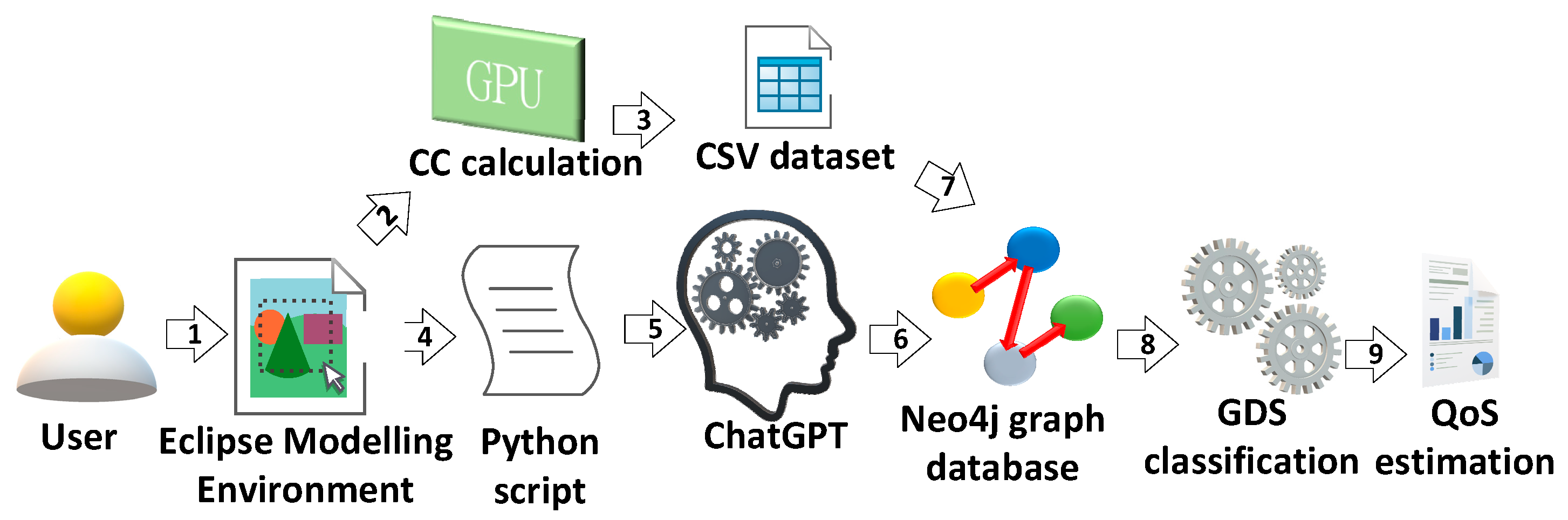
3.4. Approach Overview

Figure 4 depicts the summarized workflow behind the proposed approach for model-driven QoS estimation, leveraging Neo4j and aided by ChatGPT.

A GUI-enabled modeling tool was automatically generated within the Eclipse integrated development environment (IDE) based on our EMF meta-models: (1) the prediction problem representation [22] (illustrated in a customized, higher-level form in Figure 5), and (2) the network plan model [16]. Apart from the network infrastructure and environment details described in [16], the user also has to provide the following information required for data import and ChatGPT-aided Neo4j query generation: (1) the path of the comma-separated value (CSV) dataset file, (2) selection of the columns from the CSV files to be considered, and (3) identification of the input and output (target) variables for the selected columns. After that, Python script, relying on the PyEcore [31] library for enabling Ecore model support in the Python programming language, was used in order to extract the required parameter values from the user-created model. Furthermore, in order to construct the dataset, the CC was calculated using the previously derived expression relying on graphics hardware, as it significantly reduces the execution time thanks to loop parallelization compared to the CPU-only approach [32].

The parameters were further leveraged in order to parametrize the prompts that were sent to the ChatGPT service using the script in Figure 3. The outputs of this Python script were the following: (1) a cypher query for CSV data import into Neo4j (structured as in Row 1 in Table 3); (2) a Neo4j procedure call for the generation of a corresponding graph database based on the provided CSV (structured as in Row 2 in Table 3); (3) a Neo4j call to the GDS library for the training of the desired QoS estimation model (Row 3 in Table 3). The patterns for each of the prompts that were used for code generation are given as follows:

Import data prompt: Generate Neo4j command for importing csv file entitled {model.fileName} with following fields: {model.input_variable1, … model.input_variableN, model.target}.

Graph construction prompt: Generate Neo4j query for graph construction in case of following fields: {model.input_variable1, … model.input_variableN, model.target}.

Classifier train prompt: Generate Neo4j GDS classification train command for inputs: {model.input_variables} and output: {model.target} for graph {dataset.fileName}.

Placeholders that were parametrized from the user-provided model instance are given in Italic font within brackets. Therefore, an example of the classification query generation process in our case study is based on the following prompt:

Generate Neo4j GDS classification train command for inputs: CC, BsId, AreaId, NUsers, Season and output QoS for graph qos_predict.

Based on this prompt, ChatGPT generated the following GDS classification command, as shown in Figure 6.

3.5. Simulations and Evaluation

In this paper, we present a machine learning-based method that aims to estimate the degree of quality of service (QoS) relying on a classification algorithm, considering the previously calculated CC value as one of the model inputs. Apart from this value, several more factors were taken into account as well: (1) base station ID—identifier of the infrastructure unit responsible for a given area, (2) area ID—identifier used to distinguish the region of interest, (3) service consumers—the count of users in the considered area, and (4) season—an ID number corresponding to the part of the year. Additionally, the output of the predictive model represents a label, which is a categorical value: 1—malfunction/anomaly; 2—insufficient; 3—acceptable; 4—high. Therefore, the problem is considered as multilabel classification.

Table 4. QoS prediction dataset layout.

Variable	Description	Data Type	Role
CC	Channel capacity	Float	Input
BsId	Base station identifier	Integer	Input
AreaId	Identifier of area covered by base station	Integer	Input
Nusers	Number of users within the observed area	Integer	Input
Season	Number denoting part of year	Integer [0–3]	Input
QoS	Estimation of QoS value	Integer [1–4]	Output

gives the structure of the underlying dataset header used for the model training, exported from our simulation environment [16,32].

In order to evaluate the proposed method, a dataset counting 100,000 records was used, split into training and test subsets (75 vs. 25%). For execution, a laptop with the following specifications was used: Intel i5-10300H, 2.5 GHz, quad-core CPU, 32 GB of DDR4 RAM, and M1 SSD. Regarding the evaluation, it was analyzed from the perspectives of three different indicators: (1) prediction performance of the classification model, (2) processing time, and (3) simulation workflow speed-up compared to the manual approach without automation tools. In

Table 5. Simulations and approach evaluation.

Aspect	Component	Condition	Result
Classification	Predictor model Neo4j	Learning rate: 0.001 75% training data 25% testing data	F1—0.95 Ac—0.98
Processing time	Import CSV	100,000 records, 6 features	5.5 min
	Train		11.2 s
	Prompt construction		0.12 s
	ML query generation	Approach	Auto	Manual
		Import data	4.32 s	154 s
		Graph construction	4.76 s	467 s
		Classification	5.13 s	643 s
Acceleration	Model creation	User-created in Eclipse tool	296 s
	Query generator	ChatGPT generation	3.48 s
	Query manual	High-skill	154 + 467 + 643
			Total	1264 s
	Speed-up	Manual/ Auto	4.07 (times)

, the columns have the following meanings: (1) aspect of evaluation—the value of interest used for the estimation of the result, (2) considered component under evaluation, (3) parameters relevant to the simulation conditions and the environment, and (4) achieved results and outcomes. For the processing time, the three main steps were considered: CSV import, Neo4j graph construction, and GDS classification command.

Figure 7 illustrates the inputs and outputs of the experiments, as we started from the Ecore model instance based on the meta-model from Figure 5, imported the dataset in graph node form, and finished with QoS estimation thanks to the classification performed by the GDS library within the Neo4j software environment Neo4j Desktop (version 1.5.8) [33].

According to the achieved results, the proposed classification method for QoS estimation shows promising results regarding both the prediction performance (high accuracy) and execution speed. Considering the other approaches to QoS estimation, and taking into account the network performance metrics, it outperformed the Pytorch-based implementation from [16,22], resulting in both faster execution speed and higher accuracy compared to deep neural networks, which are more complex but less efficient for classification tasks based on few numeric values. Furthermore, compared to Weka-based classification implementation in the Java programming language using a level crossing rate [34], it outperformed all the methods in accuracy, but it required a longer overall execution time. This can be explained by the overhead of the data import and graph construction in the Neo4j graph database environment.

Regarding code generation, the ChatGPT-based Neo4j query generation time is about 1 s. Prompt construction based on a user-defined model is an order of magnitude faster. The longest execution time for query generation was in the case of the GDS classification command. Compared to the traditional approach using model-driven code generation [22], this method is slower, as it relies on ChatGPT’s huge LLM and internet service. However, this approach brings additional value, as ChatGPT is pre-trained on a huge number of textual documents and can be further specialized using proper prompts and context.

Unlike in traditional workflows, it is not required to develop a new code generation algorithm each time the simulation setup, the underlying machine learning technology, or the data format is changed. Thus, the main advantages of adopting ChatGPT in such a manner is the adaptability and extendibility.

4. Conclusions and Future Work

In this paper, an analysis of the multi-branch SC receiver under the influence of η-µ multipath fading and CCI with η-µ distribution is presented. Calculations with precision up to fifth significant digit were achieved. Based on the derived expression for channel capacity, some graphs are plotted with the signal-to-co-channel interference ratio. This provides better insight into the impact of the environmental parameters.

In the second part of the paper, we utilized the derived expression of the channel capacity for the QoS determination based on a classification model built within the Neo4j graph database ecosystem. The proposed model achieved high accuracy, reaching up to 98%.

Moreover, we integrated the QoS estimation within our simulation workflow for network planning, where ChatGPT was used to automatize the steps related to Neo4j query construction. Thereafter, thanks to prompt construction using a model-driven approach, a significant increase in the speed (more than 4 times) of the simulation workflow was achieved compared to the manual setup. The main advantage of ChatGPT is in its flexibility and dynamic customization, leveraging prompt engineering methods, rather than re-training a model with additional data.

In future work, we plan to further investigate the potential of ChatGPT for fading-type classification, taking into account real values measured in simulation conditions. Furthermore, considering the novel approaches to the performance of wireless networks, it can be found that non-Markovianity shows great potential in communication security enhancement according to the recent literature [35,36]. Additionally, the phase modulation of coherent states plays an important role in quantum communication channels [37], while the use of probabilistic noiseless linear amplifiers both at the encoding and decoding stages in cases where the information is coded on phase shifts represents a promising direction [38]. Therefore, possible future research directions might consider focusing on security aspects and the adoption of quantum communication channels, together with the corresponding AI techniques that would make such solutions more efficient.

References

1. Simon, M.K.; Alouini, M.-S. Digital Communications Over Fading Channels, 2nd ed.; John Wiley and Sons: New York, NY, USA, 2005. [Google Scholar]
2. Yacoub, M.D. The η-µ distribution: A general fading distribution. In Proceedings of the 52nd Vehicular Technology Conference VTC2000, Boston, MA, USA, 24–28 September 2000; pp. 872–877. [Google Scholar] [CrossRef]
3. Yacoub, M.D. The κ-μ distribution and the η-µ distribution. IEEE Antennas Propag. Mag. 2007, 49, 68–81. [Google Scholar] [CrossRef]
4. Ermolova, N.Y. Moment generating functions of the generalized η-µ and k-μ distributions and their applications to performance evaluations of communication systems. IEEE Commun. Lett. 2008, 12, 502–504. [Google Scholar] [CrossRef]
5. Morales-Jimenez, D.; Paris, J.F. Outage probability analysis for η-µ fading channels. IEEE Commun. Lett. 2010, 14, 521–523. [Google Scholar] [CrossRef]
6. Das, P.; Subadar, R. Performance of L-MRC receiver over exponentially correlated η-µ fading channels. Adv. Wirel. Mob. Commun. 2017, 10, 171–181. [Google Scholar]
7. Srinivasan, M.; Kalyani, S. Analysis of MRC with η-µ co-channel interference. IEEE Trans. Veh. Technol. 2020, 69, 738–745. [Google Scholar] [CrossRef]
8. Morales-Jimenez, D.; Paris, J.F.; Lozano, A. Outage probability analysis for MRC in η-µ fading channels with co-channel interference. IEEE Commun. Lett. 2012, 16, 674–677. [Google Scholar] [CrossRef]
9. Krstic, D.; Suljovic, S.; Petrovic, N.; Minic, S. GPU-enabled framework for modelling, determination and simulation the LCR of mobile networks in smart cities limited by η-µ distributed fading and interference. In Proceedings of the SpliTech 2021—6th International Conference on Smart and Sustainable Technologies, Bol, Croatia, 8-11 September 2021. [Google Scholar] [CrossRef]
10. Da Costa, D.; Filho, J.S.S.; Yacoub, M.D.; Fraidenraich, G. Second-order statistics of η-µ fading channels: Theory and applications. IEEE Trans. Wirel. Commun. 2008, 7, 819–824. [Google Scholar] [CrossRef]
11. Gvozdarev, A.S. Capacity analysis of the fluctuating double-Rayleigh with line-of-sight fading channel. Phys. Commun. 2022, 55, 101939. [Google Scholar] [CrossRef]
12. Kansal, V.; Singh, S. Analysis of effective capacity over Beaulieu-Xie fading model. In Proceedings of the 2017 IEEE International WIE Conference on Electrical and Computer Engineering (WIECON-ECE), Dehradun, India, 18–19 December 2017. [Google Scholar] [CrossRef]
13. Smilic, M.M.; Jaksic, B.S.; Milic, D.N.; Panic, S.R.; Spalevic, P.C. Channel capacity of the macrodiversity SC system in the presence of kappa-mu fading and correlated slow Gamma fading. Facta Univ. Ser. Electron. Energetics 2018, 31, 447–460. [Google Scholar] [CrossRef]
14. Milic, D.; Stanojčić, S.; Popovic, Z.; Stefanovic, D.; Petrovic, I. Performance analysis of EGC combining over correlated Nakagami-m fading channels. Serbian J. Electr. Eng. 2012, 9, 293–300. [Google Scholar] [CrossRef]
15. Mitrovic, Z.J.; Nikolic, B.Z.; Ðordjevic, G.T.; Stefanovic, M. Influence of imperfect carrier signal recovery on performance of SC receiver of BPSK signals transmitted over alfa-mi fading channel. Electronics 2009, 13, 58–62. [Google Scholar]
16. Krstic, D.; Petrovic, N.; Al-Azzoni, I. Model-driven approach to fading-aware wireless network planning leveraging multi-objective optimization and deep learning. Math. Probl. Eng. 2022, 2022, 4140522. [Google Scholar] [CrossRef]
17. Gradshteyn, I.S.; Ryzhik, I.M. Tables of Integrals, Series and Products, 7th ed.; Elsevier: Amsterdam, The Netherlands; Academic Press: Cambridge, MA, USA, 2007. [Google Scholar]
18. Suljović, S.; Krstić, D.; Bandjur, D.; Veljković, S.; Stefanović, M. Level crossing rate of macro-diversity system in the presence of fading and co-channel interference. In Revue Roumaine des Sciences Techniques; Romanian Academy: Bucharest, Romania, 2019; Volume 64, pp. 63–68. [Google Scholar]
19. Graph Database Concepts. Available online: https://neo4j.com/docs/getting-started/current/graphdb-concepts/ (accessed on 18 July 2023).
20. Cypher Query Language. Available online: https://neo4j.com/developer/cypher/ (accessed on 18 July 2023).
21. The Neo4j Graph Data Science Library Manual v2.4. Available online: https://neo4j.com/docs/graph-data-science/current/ (accessed on 18 July 2023).
22. Petrovic, N.; Al-Azzoni, I.; Krstic, D.; Alqahtani, A. Base station anomaly prediction leveraging model-driven framework for classification in Neo4j. In Proceedings of the International Conference on Broadband Communications for Next Generation Networks and Multimedia Applications, CoBCom 2022, Graz, Austria, 12–14 July 2022. [Google Scholar] [CrossRef]
23. Node Classification. Available online: https://neo4j.com/docs/graph-data-science/current/algorithms/ml-models/node-classification/ (accessed on 18 July 2023).
24. Kalla, D.; Smith, N. Study and analysis of Chat GPT and its impact on different fields of study. Int. J. Innov. Sci. Res. Technol. 2023, 8. Available online: https://ssrn.com/abstract=4402499 (accessed on 18 July 2023).
25. Wang, J.; Liu, Z.; Zhao, L.; Wu, Z.; Ma, C.; Yu, S.; Dai, H.; Yang, Q.; Liu, Y.; Zhang, S.; et al. Review of large vision models and visual prompt engineering. arXiv 2023, arXiv:2307.00855. [Google Scholar]
26. Petrović, N.; Al-Azzoni, I. Model-driven smart contract generation leveraging ChatGPT. ICSEng 2023, 761, 1–10. [Google Scholar] [CrossRef]
27. Brambilla, M.; Cabot JWimmer, M. Model-Driven Software Engineering in Practice, 2nd ed.; Morgan & Claypool Publishers: San Rafael, CA, USA, 2017. [Google Scholar]
28. Rodrigues da Silva, A. Model-driven engineering: A survey supported by the unified conceptual model. Comput. Lang. Syst. Struct. 2015, 43, 139–155. [Google Scholar] [CrossRef]
29. Steinberg, D.; Budinsky, F.; Paternostro, M.; Merks, E. EMF: Eclipse Modeling Framework; Addison-Wesley Professional: Boston, MA, USA, 2008; Chapter 5. [Google Scholar]
30. Eclipse Modeling Framework (EMF). Web Reference. Available online: https://www.eclipse.or modeling/emf/ (accessed on 4 August 2023).
31. PyEcore: A Pythonic Implementation of the Eclipse Modeling Framework. Available online: https://github.com/pyecore/pyecore (accessed on 21 July 2023).
32. Petrović, N.; Vasić, S.; Milić, D.; Suljović, S.; Koničanin, S. GPU-supported simulation for ABEP and QoS analysis of a combined macro diversity system in a Gamma-shadowed k-µ fading channel. Facta Univ. Ser. Electron. Energetics 2021, 34, 89–104. [Google Scholar] [CrossRef]
33. Neo4j Desktop. Available online: https://neo4j.com/docs/desktop-manual/current/ (accessed on 21 July 2023).
34. Suljovic, S.; Krstic, D.S.; Nestorovic, G.; Petrovic, N.N.; Minic, S.; Gurjar, D.S. Using level crossing rate of selection combining receiver damaged by Beaulieu-Xie fading and Rician co-channel interference with a purpose of machine learning QoS level prediction. Elektron. Ir Elektrotechnika 2023, 29, 68–73. [Google Scholar] [CrossRef]
35. Vasile, R.; Olivares, S.; Paris, M.A.; Maniscalco, S. Continuous-variable quantum key distribution in non-Markovian channels. Phys. Rev. 2011, 83, 042321. [Google Scholar] [CrossRef]
36. Teklu, B.; Bina, M.; Paris, M.G.A. Noisy propagation of Gaussian states in optical media with finite bandwidth. Sci. Rep. 2022, 12, 11646. [Google Scholar] [CrossRef] [PubMed]
37. Adnane, H.; Teklu, B.; Paris, M.G.A. Quantum phase communication channels assisted by non-deterministic noiseless amplifiers. J. Opt. Soc. Am. B 2019, 36, 2938–2945. [Google Scholar] [CrossRef]
38. Trapani, J.; Teklu, B.; Olivares, S.; Paris, M.G.A. Quantum phase communication channels in the presence of static and dynamical phase diffusion. Phys. Rev. A 2015, 92, 012317. Available online: https://journals.aps.org/pra/abstract/10.1103/PhysRevA.92.012317 (accessed on 3 August 2023). [CrossRef]
39. DiDonato, A.R.; Jarnagin, M.P. The efficient calculation of the incomplete Beta-function ratio for half- integer values of the parameters a, b. Math. Comput. 1967, 21, 652–662. [Google Scholar] [CrossRef]
40. Abramowitz, M.; Stegun, I.A. (Eds.) Confluent Hypergeometric Functions. Ch. 13. In Handbook of Mathematical Functions with Formulas, Graphs, and Mathematical Tables; Dover: New York, NY, USA, 1972; pp. 503–515. [Google Scholar]
41. Huang, H.C.; Yuan, C. Ergodic capacity of composite fading channels in cognitive radios with series formula for product of κ-μ and α-μ fading distributions. IEICE Trans. Commun. 2020, 103, 458–466. [Google Scholar] [CrossRef]
42. Ribičić Penava, M.; Škrobar, D. Gamma and Beta functions. Osječki Mat. List 2015, 15, 93–111. (In Croatian) [Google Scholar]
Figure 1. Normalized channel capacity versus the output SIR for different values of fading and CCI parameters µ1 and µ2.
Electronics 12 04088 g001
Figure 2. Normalized channel capacity for different values of fading and CCI parameters η1 and η2 and number of branches L.
Electronics 12 04088 g002
Figure 3. Excerpt of Python code for programmatic access to ChatGPT service.
Electronics 12 04088 g003
Figure 4. ChatGPT-aided classification workflow for QoS estimation using Neo4j and ChatGPT: (1) modeling; (2) network model; (3) CC value; (4) prediction problem model; (5) ChatGPT prompt; (6) cypher queries; (7) data import and graph construction; (8) GDS classification query; (9) predictions.
Electronics 12 04088 g004
Figure 5. Prediction problem meta-model customization for Neo4j.
Electronics 12 04088 g005
Figure 6. Example of ChatGPT code generation in case of GDS classifier training command.
Electronics 12 04088 g006
Figure 7. Experiment illustration: from Ecore model instance to classification in Neo4j Desktop (version 1.5.8) [33] graph database software environment.
Electronics 12 04088 g007