Optimal Pattern Synthesis of Linear Array Antennas Using the Nonlinear Chaotic Grey Wolf Algorithm

Abstract

The grey wolf optimization (GWO) algorithm is a new nature-inspired meta-heuristic algorithm inspired by the social hierarchy and hunting behavior of grey wolves. In this paper, the GWO algorithm is improved to overcome previous shortcomings of being easily trapped in local optima and having a low convergence rate. The proposed enhancement of the GWO algorithm utilizes logistic-tent double mapping to generate initialized populations, which enhances its global search capability and convergence rate. This improvement is called the nonlinear chaotic grey wolf optimization (NCGWO) algorithm. The performance of the NCGWO algorithm was evaluated with four representative benchmark functions. Then, the NCGWO algorithm was applied to perform an optimal pattern synthesis of linear array antennas (LAAs) using two distinct approaches: optimizing the amplitudes of the antenna currents while preserving uniform spacing and optimizing the positions of the antennas while assuming uniform excitation. To validate the effectiveness of the proposed approach, the results obtained by the NCGWO algorithm were compared with those obtained by other intelligent algorithms. Additionally, the NCGWO algorithm was applied to a more complex planar antenna array to further validate its performance. Our results demonstrate that the NCGWO algorithm exhibits superior performance regarding electromagnetic optimization problems compared to widely recognized algorithms.

1. Introduction

Array antennas are indispensable in present-day Wi-Fi verbal exchange systems. Compared to a single antenna, array antennas have greater directivities, greater gains, and higher competencies in beam control and null placement [1], which make them a crucial component in implementing fifth-generation (5G) and satellite communication systems [2]. Since environmental friendliness has become a significant theme of the current era, technological innovation is the ultimate solution to a green and sustainable system. A new track is opened by array antennas. For example, compared with the U.S. Arecibo array, the 500 m Aperture Spherical Radio Telescope of China has a 64% larger aperture, 2.5 times higher sensitivity, and 10 times higher comprehensive performance, and it can detect up to 13.7 billion light years away. Consequently, the efficiency enhancements of array antennas are apparent.

In a broader context, array antenna elements can be structured in various configurations: linear, planar, and three-dimensional. When focusing on the pattern synthesis for linear array antennas (LAAs), there are two different types of LAAs: a uniform array with equal spacing and a nonuniform array. Furthermore, in the realm of planar arrays, the rectangular configuration stands out as a prevalent choice due to its geometric attributes and inherent traits [3]. Placing null placements in particular directions and reducing the sidelobe level (SLL) are essential methods to prevent the interference of array antennas [4]. However, in the pattern synthesis of array antennas, attaining a combination of low SLL, null control, and narrow main beam is challenging due to their inherent mutual constraints. The mutual coupling of array elements can affect the efficiency of array antennas, so the coupling effect between the elements should also be considered in the design to ensure better performance of the array antennas [2,5,6].

Previously, the conventional Taylor’s method was employed for pattern synthesis with low SLL [7]. With the development of mathematics, several evolutionary algorithms have proven effective in the electromagnetic field, many of which are applied in the pattern synthesis of array antennas, such as the grey wolf optimization (GWO) algorithm [8], particle swarm optimization (PSO) algorithm [9], biogeography-based optimization (BBO) algorithm [10], firefly algorithm (FA) [11], genetic algorithm (GA) [12], difference evolution (DE) algorithm [13], exponential chaotic differential evolution (ECDE) [14], grasshopper optimization algorithm (GOA) [15], quantum particle swarm optimization (QPSO) algorithm [16], spider monkey optimization (SMO) algorithm [17], mayfly algorithm (MA) [18], wind-driven optimization (WDO) algorithm [19], invasive weed (IWO) algorithm [20], and atom search optimization (ASO) algorithm [21]. These algorithms have demonstrated commendable performance within their capabilities; however, the growing demand for anti-interference in information transmission has underscored the necessity for continuous research in the realm of intelligent antenna optimization. Hence, research on the enhancement of the current and new optimization methods has become active recently.

The GWO algorithm was employed to optimize LAAs to synthesize optimal radiation patterns. The primary objective was to achieve an array pattern with a minimal SLL and place nulls in the specified directions. The GWO algorithm was successfully utilized to accomplish this goal [22]. The Improved Grey Wolf (IGWO) algorithm was previously utilized to optimize a uniform LAA for optimal pattern synthesis [23]. In this study, the original GWO algorithm has been reworked to an NCGWO algorithm, logistic-tent double mapping is adopted to generate initialized populations, and a convergence factor formula of the Gaussian function is used to enhance the overall performance of the GWO algorithm. The work proposes using the NCGWO algorithm for the pattern synthesis of LAAs and planar arrays.

The remainder of this study is structured as follows: Section 2 provides a comprehensive description of the GWO algorithm. Section 3 outlines the enhancements and specific formulations of the NCGWO algorithm. Section 4 compares various algorithms based on test functions. Then, Section 5 and Section 6 describe the array factor expressions of array antennas and data results, respectively. Finally, Section 7 draws the conclusion.

2. GWO Algorithm

The GWO algorithm imitates the observed natural hierarchy of leadership and hunting mechanism in grey wolves. Figure 1 shows the hierarchy of grey wolves. There are three steps in hunting: searching for prey, encircling the prey, and attacking the prey.

The α wolf is the leader, and its decision making encompasses the hunting behavior, habitat selection, and food distribution. Other wolves obey the orders of the α wolf. The second layer of the pyramid is called the β wolf, which is the successor of the α wolf. The third level is δ, which follows the commands of the α and β wolves. Older α and β wolves also descend to the level of δ wolves. The bottom layer, i.e., the ω wolf, is responsible for balancing the relationships within the population. This hierarchical structure ensures efficient and effective decision making within the pack. Grey wolves are known for their cooperative hunting behavior, where the β wolf and δ wolf engage in pursuing, encircling, and attacking prey under the guidance of the α wolf [23]. Figure 2 illustrates how an ω wolf adjusts its location within a 2D space by following the guidance of the α, β, and δ wolves.

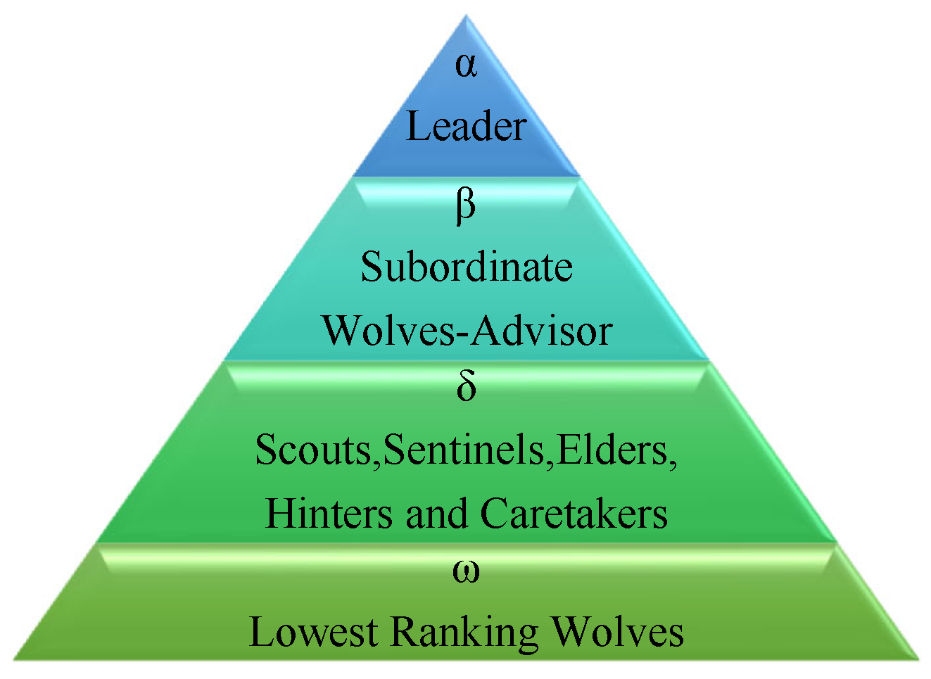
2.1. Social Hierarchy

To optimize the search using the GWO algorithm, the α solution is designated as the most appropriate solution, which is followed by the β and δ solutions. Any other potential solution is categorized as an ω solution to align with the progression of the three prior solutions since the search process of the algorithm is guided by them [23].

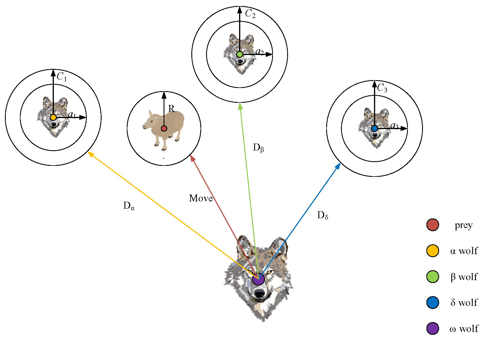
2.2. Encircling Prey

Upon the detection of a prey (t = 1), the first iteration commences. Subsequently, the ω wolves, which are guided by the α, β, and δ wolves, pursue and ultimately surround the prey. The following equations describe the encircling behavior:

$${\overrightarrow{D}}_{\alpha }=\left|{\overrightarrow{C}}_1•{\overrightarrow{X}}_{\alpha }-\overrightarrow{X}\left(t\right)\right|$$

(1)

$${\overrightarrow{D}}_{\beta }=\left|{\overrightarrow{C}}_2•{\overrightarrow{X}}_{\beta }-\overrightarrow{X}\left(t\right)\right|$$

(2)

$${\overrightarrow{D}}_{\delta }=\left|{\overrightarrow{C}}_3•{\overrightarrow{X}}_{\delta }-\overrightarrow{X}\left(t\right)\right|$$

(3)

where ${\overrightarrow{D}}_i\left(i=\alpha ,\beta ,\delta \right)$ is the wolf’s distance from the prey; the location vector of the prey is defined by ${\overrightarrow{X}}_i\left(i=\alpha ,\beta ,\delta \right)$, the location vector of a grey wolf at iteration t is $\overrightarrow{X}\left(t\right)$, and the coefficient vector ${\overrightarrow{C}}_i\left(i=1,2,3\right)$ represents random disturbances in the positions of the wolves. These coefficients are calculated as follows:

$${\overrightarrow{C}}_i=2{\overrightarrow{r}}_i$$

(4)

where ${\overrightarrow{r}}_i$ is a random vector in [0, 1].

2.3. Hunting and Attacking Prey

Grey wolves have a remarkable ability to discern the location of their prey and orchestrating its encirclement. In the pursuit and assault of a prey, the role of the leader is typically assumed by the α, which is occasionally accompanied by the participation of the β and δ. Conventionally, it is widely acknowledged that the α, β, and δ individuals are the most experienced hunters and have superior knowledge regarding potential prey positions. Other members of the wolf pack follow the directives given by the α, β, and δ. As a result, the foremost three optimal solutions are conserved, which compels the remaining search agents to adjust their positions by the coordinates of the leading search agent. To elucidate this concept, the following formula is proposed [8].

The positions of the α, β, and δ wolves are individually computed as follows:

$${\overrightarrow{X}}_1={\overrightarrow{X}}_{\alpha }-{\overrightarrow{A}}_1•{\overrightarrow{D}}_{\alpha }$$

(5)

$${\overrightarrow{X}}_2={\overrightarrow{X}}_{\beta }-{\overrightarrow{A}}_2•{\overrightarrow{D}}_{\beta }$$

(6)

$${\overrightarrow{X}}_3={\overrightarrow{X}}_{\delta }-{\overrightarrow{A}}_3•{\overrightarrow{D}}_{\delta }$$

(7)

where ${\overrightarrow{X}}_i\left(i=1,2,3\right)$ are the positions of the α, β, and δ wolves; ${\overrightarrow{X}}_i\left(i=\alpha ,\beta ,\delta \right)$ is the position vector of the prey; ${\overrightarrow{A}}_i\left(i=1,2,3\right)$ is the vector coefficient; and ${\overrightarrow{D}}_i\left(i=\alpha ,\beta ,\delta \right)$ is the wolf’s distance from the prey.

$\overrightarrow{A}$ is the vector coefficient; when $\left|\overrightarrow{A}\right|>1$, the grey wolf expands its search to find food, which corresponds to a global search; when $\left|\overrightarrow{A}\right|<1$, the grey wolf narrows the envelope, which corresponds to a local search. $\overrightarrow{A}$. is calculated as follows:

$$\overrightarrow{A}=2a\overrightarrow{r}-a$$

(8)

where $\overrightarrow{r}$ is a vector of random values of 0–1, a is the convergence factor, and a is a linearly decreasing variable that starts at 2 and approaches 0 with each iteration. This is represented in the GWO algorithm as follows:

$$a=2-2\left(\frac{t}{T_{\max }}\right)$$

(9)

where t is the number of current iterations, and $T_{\max }$ is the maximum number of iterations. In the original GWO, the positions of the grey population in the next generation can be obtained by the average positions of the α, β, and δ wolves. These are calculated as follows:

$$\stackrel{\rightharpoonup }{X}(\mathrm{t}+1)=\frac{{\stackrel{\rightharpoonup }{X}}_1+{\stackrel{\rightharpoonup }{X}}_2+{\stackrel{\rightharpoonup }{X}}_3}{3}$$

(10)

3. Nonlinear Chaotic Grey Wolf Optimization (NCGWO) Algorithm

The NCGWO algorithm is based on the GWO algorithm with two improvements: the initial population is generated by introducing logistic-tent double mapping and the convergence factor based on the Gaussian function is enhanced. This section describes the improvements and specific expressions of the NCGWO algorithm.

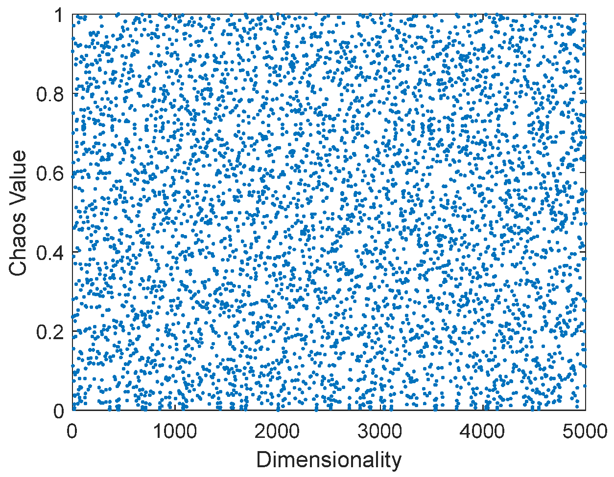
3.1. Logistic-Tent Double Mapping

Logistic mapping is a single-peaked mapping, which perfectly inherits the advantages of randomness and the initial value of sensitivity inherent in chaos [24]. The logistic mapping is expressed as follows:

$$X_{n+1}=U{X}_n(1-X_n)$$

(11)

where $X_n$ is the iteration result $X_n\in \left(0,1\right)$, and $U$ is a parameter $U\in \left(0,4\right)$.

The tent chaotic system is a segmented linear one-dimensional mapping with chaotic properties, uniform probability density and power spectral density, and a relatively good autocorrelation [25]. It is mathematically derived as follows:

$$X_{n+1}=\left\{\begin{array}{l}a{x}_n,0\le x_n<0.5\\ a\left(1-x_n\right),0.5\le x_n\le 1\end{array}\right.$$

(12)

where $x$ is the system variable and $x\in [0,1]$, and a control parameter is between (0 and 1) and it is $a\ne 0.5$ when the system is chaotic.

Compared to logistic mapping, tent mapping has a uniform probability density, a uniform power spectral density, ideal correlation properties, and a faster iteration speed [26].

This study uses the logistic-tent double mapping [27], which combines the complex chaotic dynamics properties of the logistic mapping with a faster iteration speed, greater autocorrelation, and the applicability to many sequences of the tent chaotic system. Its mathematical formulation is as follows:

$$X_{n+1}=\left\{\begin{array}{l}\left[r{x}_n\left(1-x_n\right)+\frac{\left(4-r\right)}{2}{x}_n\right]\mathrm{mod}1,\mathrm{if}{x}_n<0.5\\ \left[r{x}_n\left(1-x_n\right)+\frac{\left(4-r\right)\left(1-x_n\right)}{2}\right]\mathrm{mod}1,\mathrm{if}{x}_n\ge 0.5\end{array}\right.$$

(13)

where $X$ is the system variable, r is the control parameter $x\in \left[0,1\right]$, and $r\in \left[0,4\right]$. In this study, the logistic-tent double mapping is used for initialization, so that the initial solutions are distributed as uniformly as possible in the solution space, as shown in Figure 3.

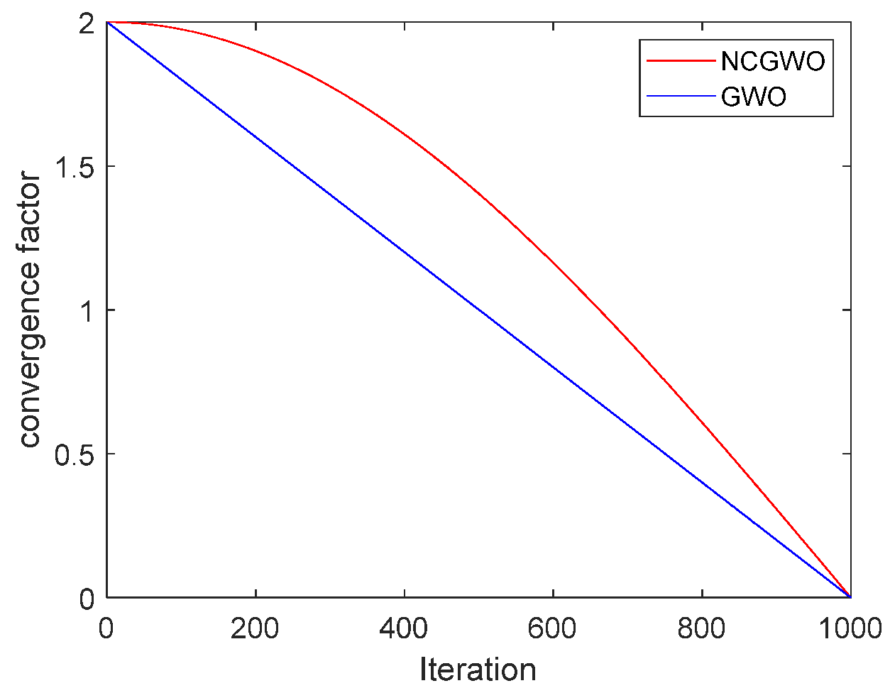
3.2. Nonlinear Variable Speed Convergence Factor

All population intelligence optimization algorithms have the problem of balancing the global search ability and local search ability. A strong global search ability can ensure the diversity of the population, and a strong local search ability can ensure a locally accurate search and accelerate the convergence of the algorithm. Therefore, the importance of balancing the global search ability and local search ability in the GWO algorithm is self-evident.

The convergence factor of the GWO algorithm linearly decreases from 2 to 0 over successive iterations. This decrease during continuous convergence renders a strategy of linearly decreasing the convergence factor that is inadequate for holistically capturing the intricate optimization search dynamics, as noted by [28]. Accordingly, this study introduces a convergence factor by exponential attenuation:

$$a=H{e}^{-\left(t^2/2M^2\right)}-(H-2)$$

(14)

where e is the natural exponent; t is the current iteration number; M is the maximum number of iterations; H is the coefficient vector, which is used to adjust the convergence factor to make it nonlinearly decrease from 2 to 0. Figure 4 shows the nonlinear relationship between the improved convergence coefficient and the number of iterations.

Based on the data plotted in Figure 4, when the number of iterations increases, the improved convergence coefficient nonlinearly decreases. The decay rate is lower during the initial stages of the algorithm to enhance the search for the global optimal solution, while it accelerates in the later stages to achieve a more precise localization of the local optimal solution. This approach effectively balances the search capabilities for both global and local solutions [29].

Based on this description,

Table 1. Comparison of the GWO and NCGWO improvement points.

	NCGWO	GWO
Number 1	Logistic-tent double mapping generating initial populations	Randomly generated initial populations
Formula	$X_{n+1}=\left\{\begin{array}{l}\left[r{x}_n\left(1-x_n\right)+\frac{\left(4-r\right)}{2}{x}_n\right]\mathrm{mod}1,\mathrm{if}{x}_n<0.5\\ \left[r{x}_n\left(1-x_n\right)+\frac{\left(4-r\right)\left(1-x_n\right)}{2}\right]\mathrm{mod}1,\mathrm{if}{x}_n\ge 0.5\end{array}\right.$	$X_{n+1}=rand\left(X_n\right)$
Reason 1	The GWO algorithm suffers from a lack of diversity in the initial population due to the random generation of individuals. This limitation hampers the algorithm’s search flexibility. To address this, logistic-tent dual chaotic mapping methods are employed to enhance the initial population’s diversity, optimizing the global search process and increasing the algorithm’s search flexibility.
Number 2	Nonlinear variable speed convergence factor	Linear convergence factor
Formula	$a=H{e}^{-\left(t^2/2M^2\right)}-(H-2)$	$a=2-2\left(\frac{t}{T_{\max }}\right)$
Reason 2	The a plays an important role in balancing the exploration and exploitation of the candidate’s individual search. The search process of the GWO algorithm is nonlinear and complicated; the linear convergence factor cannot balance the global and local search ability. The better performance would be obtained if there was a nonlinear variable speed convergence factor.

succinctly outlines the disparities between NCGWO and GWO algorithms.

3.3. NCGWO Algorithm Steps

Figure 5 shows the NCGWO implementation steps. Initially, the initial population is generated, and parameters are defined for the fitness value calculation, where the best values are stored as α, β, and δ. Subsequently, the positions are updated, which ultimately leads to the output of the optimal solution $X_{\alpha }$.

4. NCGWO Performance Analysis

The overall performance of NCGWO algorithm used to be first examined on four popular benchmark functions, which are used as metrics to consider the performances of optimization algorithms in many instances. The results were compared to those of well-known metaheuristic optimization methods such as GWO, PSO, and GA [30] (

Table 2. Benchmark function and their properties.

F	Expression	Boundaries	Optimal Solution i.e., $\mathit{f}({\mathit{x}}^{\ast })$
F1	$f(x)={\displaystyle \sum _{i=1}^D{x}_i{}^2}$	$-100\le x_i\le 100$	$x^{\ast }=\left[0,0,\dots ,0\right]f(x^{\ast })=0$
F2	$f(x)={\displaystyle \sum _{i=1}^{D-1}\left[100\left(x_{i+1}-x_i{}^2\right)+{(1-x_i)}^2\right]}$	$-30\le x_i\le 30$	$x^{\ast }=\left[1,1,\dots ,1\right]f(x^{\ast })=0$
F3	$f(x)={\displaystyle \sum _{i=1}^D\left[x_i{}^2-10\cos (2\pi x_i)+10\right]}$	$-5.12\le x_i\le 5.12$	$x^{\ast }=\left[0,0,\dots ,0\right]f(x^{\ast })=0$
F4	$f(x)=\frac{1}{4000}{\displaystyle \sum _{i=1}^D{x}_i{}^2}-{\displaystyle \prod _{i=1}^D}\cos \left(\frac{x_i}{\sqrt{i}}\right)+1$	$-100\le x_i\le 100$	$x^{\ast }=\left[0,0,\dots ,0\right]f(x^{\ast })=0$

).

Table 3. Result comparison with 50 independent runs.

Objective Function	Algorithm	Min	Mean	SD
$f_1(x)$	NCGWO	7.6893 × 10−99	2.6133 × 10−100	1.4032 × 10−99
	GWO	2.60 × 10−73	3.55 × 10−71	1.18 × 10−70
	PSO	5.01 × 10−17	5.96 × 10−15	2.54 × 10−14
	GA	2.23 × 10−31	1.3 × 10−3	0.105
$f_2(x)$	NCGWO	27.10	26.01	0.59
	GWO	34.45	36.40	0.75
	PSO	10.574	54.55	56.00
	GA	23.89	284.04	255.57
$f_3(x)$	NCGWO	0	0	0
	GWO	0	2.27 × 10−15	1.11 × 10−14
	PSO	21.89	77.89	24.37
	GA	11.94	35.97	12.26
$f_4(x)$	NCGWO	0	0	0
	GWO	0	6.24 × 10−4	2.52 × 10−3
	PSO	0	1.48 × 10−2	2.38 × 10−2
	GA	0	1.7 × 10−3	1.46 × 10−2

compares the other algorithms on the benchmark functions. Figure 6 shows the 2D graphics.

Figure 6a,b are unimodal functions, each of which contains only one optimum. Figure 6a is smooth, unimodal, strongly convex, and symmetric. Figure 6b has a very narrow ridge, the tip of the ridge is very sharp, and it runs around a parabola. Figure 6c,d are multimodal functions with many local optima but only one global optimum. Figure 6c has a large search space and many local minima, and there are millions of locally optimal solutions in this interval alone. Figure 6d is the term of the summation that produces a parabola, while the local optima are above the parabola level [31].

In this test case, each algorithm was independently executed 50 times, and the population size and maximum number of iterations were set to 100 and 1000, respectively. Table 3 shows that the NCGWO algorithm outperformed the other algorithms on test functions F1, F3, and F4, while the PSO algorithm showed a better performance on F2. However, the NCGWO algorithm consistently demonstrated superior performance across all test functions (Table 3). Therefore, we conclude that the NCGWO algorithm outperforms the GWO algorithm.

5. Array Antenna

This section presents the model and array factor of LAAs and planar arrays. The problem of optimizing the PSLL and objective function is detailed in [32].

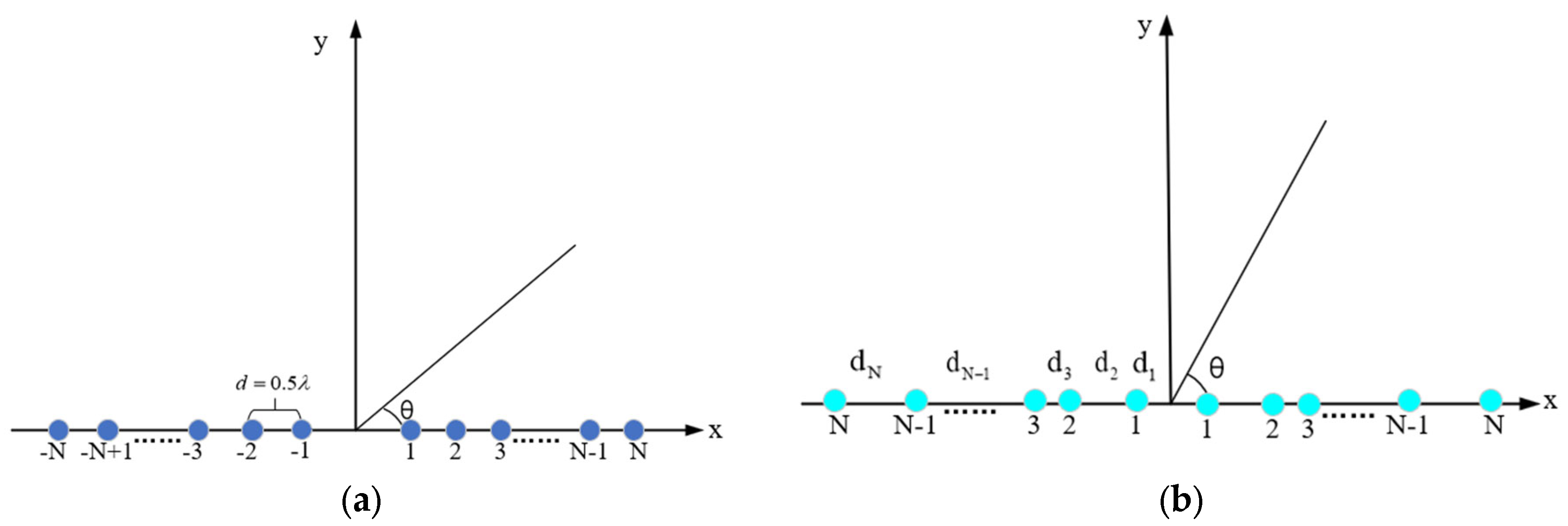
5.1. Linear Array Antennas

In this study, a uniform LAA was employed, where an equi-spaced array of 2N electric dipoles was symmetrically positioned along the x-axis (Figure 7a). The electric field in the far-field region for an electric dipole is given in Ref. [32]:

$$E\left(\theta \right)=j\frac{Idl}{4\pi }\left(\frac{e^{-jkR}}{R}\right){\eta }_{0}k\sin \theta$$

(15)

where $Idl$ is the excitation amplitude, ${\eta }_0$ is the impedance of free space, k is the free space wave number $k=2\pi /\lambda$, and $\lambda$ is the wavelength. Here, we can ignore $\left(e^{-jkR}/R\right)$, the far-field expression.

For array antennas, the field pattern $f\left(\theta \right)$ is expressed as a product of $E\left(\theta \right)$ and the array factor $F\left(\theta \right)$:

$$f\left(\theta \right)=E\left(\theta \right)\times F\left(\theta \right)$$

(16)

where the array factor of the far-field uniform linear array antenna is expressed in decibels using an equation in Ref. [33], as follows:

$$F\left(\theta \right)=2{\displaystyle \sum _{n=1}^N{I}_n}\cos \left(kd\cos \theta +{\delta }_n\right)$$

(17)

The excitation amplitude of the Nth element is represented by I, k is the wave number $k=2\pi /\lambda$,$\lambda$ is the wavelength in free space, and distance d between arrays was set to $0.5\lambda$. The variable $\theta$ is the angle between the ray direction and the array axis, and ${\delta }_n$ is the phase of the Nth element, which was set to ${\delta }_n=0$.

For the sparse linear array antenna in Figure 7b, the inter-element spacing was optimized, while the amplitude and phase were assumed to be 1 and 0, respectively. The equation for the sparse LAA array factor in Ref. [33] is

$$F\left(\theta \right)=2{\displaystyle \sum _{n=1}^N\cos \left(kd\cos \theta \right)}$$

(18)

For an even-numbered array, Equation (16) is applicable. If it is an odd-numbered array, the array factor can be obtained by adding 1 to Equation (18).

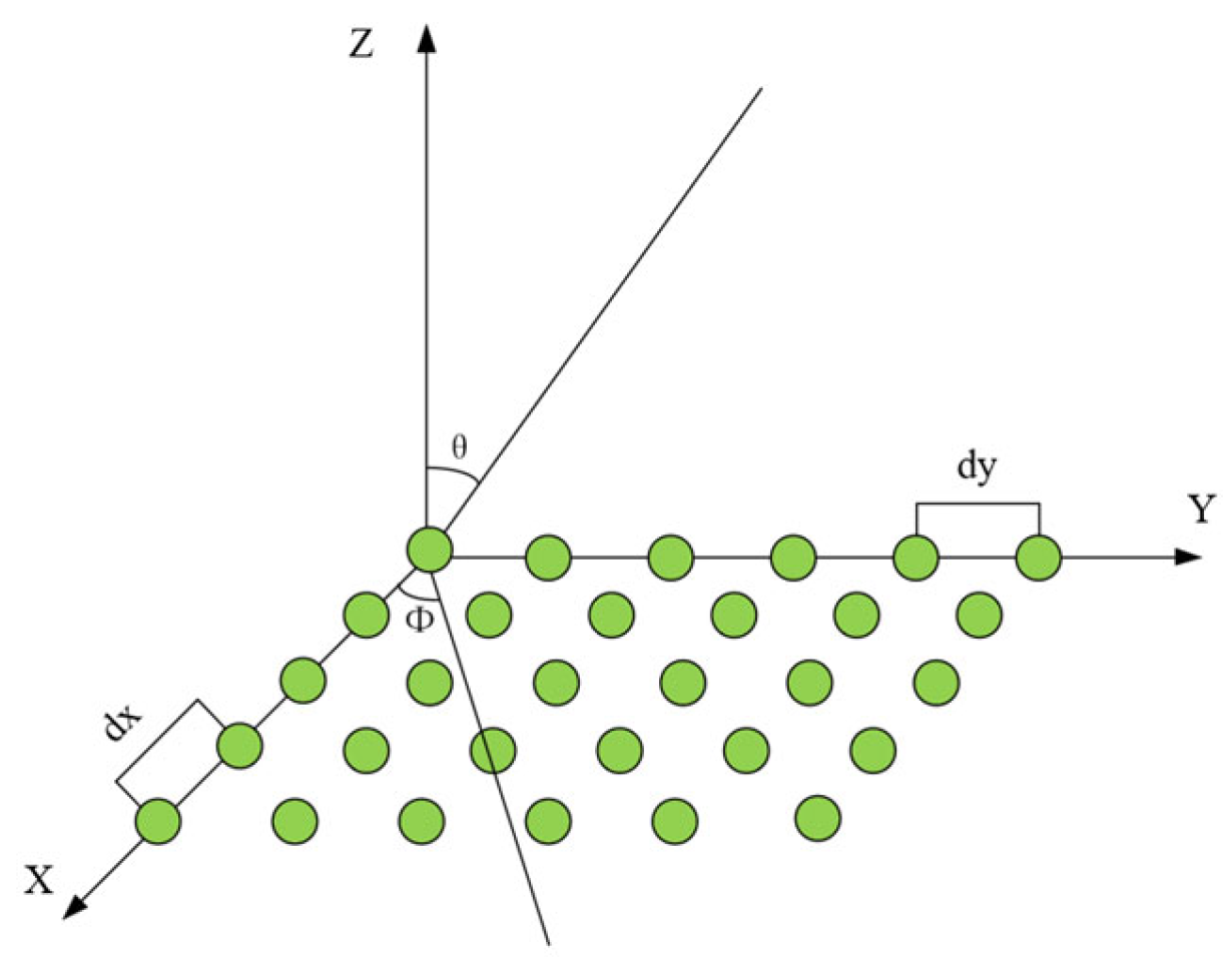
5.2. Planar Array Antenna

Planar array antennas enhance the antenna directionality compared to LAAs. In Figure 8, a rectangular planar array consists of $n=n_x•n_y$ identical antenna units, where dx and dy are the intervals between antenna units along the x and y axes, respectively. The equation for the planar array antenna pattern is expressed in Ref. [34] as follows:

$$F\left(\theta ,\phi \right)=F_x\left(\theta ,\phi \right)•F_y\left(\theta ,\phi \right)$$

(19)

$$F\left(\theta ,\phi \right)={\displaystyle \sum _{n=1}^N{I}_n{e}^{j2\pi d_x\sin \theta \cos \phi }}{e}^{j2\pi d_y\sin \theta \sin \phi }$$

(20)

where N is the total number of antenna elements in the array; $\theta$ is the elevation angle with respect to the z-axis; $\phi$ is the azimuth angle with respect to the x-axis; I is the excitation amplitude of the Nth element; d_x and d_y are the intervals between antenna units along the x- and y-axes, respectively; $d_x=d_y=0.5\lambda$; $\lambda$ is the wavelength.

5.3. Pattern Synthesis of Array Antennas

The objective is to minimize the decrease in SLL below the predicted value while maintaining a constant main lobe width of the array and achieving deep nulls in specific directions. To achieve this objective, the following fitness function was used [23]:

$$Fit={\eta }_1\left|PSLL-TPSL\right|+{\eta }_2\left|\max {\left\{F\left({\theta }_K\right)\right\}}_{k=1,\dots N_0}-DDNL\right|$$

(21)

where PSLL is the peak sidelobe level; TPSL is the target peak sidelobe level; $F({\theta }_k)$ is the direction of the kth deep null; DDNL is the desired deep null level; ${\eta }_1$ and ${\eta }_2$ are the weighting factors and subject to the condition ${\eta }_1+{\eta }_2=1$.

6. Data Analysis

6.1. Reducing the First Sidelobe Level (SLL) Nearest to the Main Lobe of a Uniform LAA

In the first example, the NCGWO algorithm was utilized to synthesize the pattern of a uniform LAA. The performance of the NCGWO algorithm was compared with that of the IGWO [23], GWO, PSO, and MA [35] algorithms. Assuming zero-phase excitation, the amplitudes of the excitation current were optimized for LAA with 2N = 10 to achieve the desired peak sidelobe level (PSLL). The main lobe width was set to ${28}^{°}$, while the sidelobe regions were $\theta =\left[0^{°},{76}^{°}\right]\cup \left[{104}^{°},180^{°}\right]$. Meanwhile, the first sidelobe, which is closest to the main lobe, was minimized within the region defined by $\theta =\left[{69}^{°},{76}^{°}\right]\cup \left[{104}^{°},111^{°}\right]$. The NCGWO algorithm was executed with a population size of 20 for 1000 iterations, which is consistent with previous studies [34].

Figure 9a depicts the array pattern obtained using the NCGWO algorithm, which was compared with the results of the IGWO, GWO, PSO, and MA algorithms. Figure 9b illustrates the iteration curves that correspond to the GWO, IGWO, and NCGWO algorithms. Evidently, the NCGWO algorithm converges to the optimal value within approximately 100 generations, whereas the GWO and IGWO algorithms require approximately 400 generations to achieve the same outcome. This outcome underscores the superior performance of the NCGWO algorithm compared to the GWO and IGWO algorithms. Figure 10 shows the 3D radiation patterns of reducing the 10-element LAA’s first SLL before and after the NCGWO optimization, which clearly demonstrates the effectiveness of the NCGWO algorithm in significantly reducing the first SLL.

Table 4. Results for a 10-element linear array antenna.

Algorithm	Optimized Amplitude Current	Peak SLL (dB)	Near SLL (dB)	Execution Time (s)
GWO	0.9531, 0.9452, 0.5549, 0.4634, 0.5083	−16.8570	−31.8400	3.1800
IGWO	1.0000, 0.8376, 0.6409, 0.4349, 0.4768	−20.2761	−31.9129	2.4520
PSO	0.9242, 0.7997, 0.6030, 0.3814, 0.4766	−19.4041	−32.4200	2.9300
MA	1.0000, 0.8585, 0.6383, 0.4253, 0.5070	−20.0367	−32.4500	9.3700
NCGWO	1.0000, 0.8645, 0.6455, 0.4105, 0.3999	−22.4420	−36.4027	0.8290

shows the optimization results in the example. The NCGWO algorithm achieved a minimized nearest SLL of −36.4027 dB and a running time of 0.8290 s. This minimized nearest SLL was lower than those of GWO, IGWO, PSO, and MA by 4.5627, 4.4898, 3.9827, and 3.9527 dB, respectively. The PSLL achieved by the NCGWO algorithm was −22.4420 dB, which was 5.585, 2.1659, 3.0379, and 2.4053 dB lower than those of GWO, IGWO, PSO, and MA, respectively.

6.2. Array Factor of a 20-Element Uniform Linear Array Antenna with a Lower Notch

In the second example, an LAA with 20 elements was considered to decrease the SLL in the sidelobe regions of $\theta =\left[0^{°},82^{°}\right]\cup \left[{98}^{°},{180}^{°}\right]$ with lower notches in the specific directions of $\theta =\left[{50}^{°},{60}^{°}\right]\cup \left[{120}^{°},{130}^{°}\right]$. The NCGWO algorithm was executed with a population size of 30 and at most 500 iterations, consistent with previous studies [36].

Figure 11a depicts the LAA pattern synthesized using the NCGWO algorithm and compares it with the results of the GWO, IGWO, GOA, and SMO algorithms. Figure 11b illustrates the iteration curves that correspond to the GWO, IGWO, and NCGWO algorithms. Although all three algorithms obtain the optimal value within 500 generations, a discernible disparity is evident in the figure. Specifically, the NCGWO algorithm demonstrates a more favorable optimal value than GWO and IGWO. Figure 12 illustrates the 3D radiation patterns of a 20-element LAA before and after the NCGWO optimization. NCGWO significantly reduces the PSLL and the notch.

Table 5. Results for a 20-element linear array antenna.

Algorithm	Optimized Amplitude Current	Peak SLL (dB)	Notch Depth (dB)	Execution Time (s)
GWO	0.8785, 0.9057, 0.8858, 0.7978, 0.6418 0.5180, 0.3663, 0.3101, 0.1407, 0.0939	−26.9677	62.6431	3.075
IGWO	0.9795, 0.9716, 0.9386, 0.7924, 0.7202 0.5613, 0.5115, 0.3950, 0.2175, 0.1190	−27.0144	−62.1436	2.5920
SMO	1.0000, 0.9990, 1.0000, 0.8360, 0.6430 0.6540, 0.4770, 0.5970, 0.2580, 0.2150	−24.1000	−56.7000	9.612
GOA	1.0000, 0.9860, 0.9900, 0.7960, 0.7360 0.5630, 0.5270, 0.4470, 0.2430, 0.1510	−27.7000	−61.2000	7.714
NCGWO	1.0000, 0.9636, 0.9417, 0.7958, 0.7000 0.5752, 0.4474, 0.3626, 0.1699, 0.1008	−28.1781	−64.3883	1.998

shows the optimization results. The results demonstrate that the NCGWO algorithm achieved a PSLL of −28.1781 dB, and the PSLL of the notch was −64.3883 dB. Compared with the reported results of the GWO, IGWO, GOA, and SMO algorithms [36], the PSLL of the NCGWO algorithm was 1.2140, 1.1637, 4.0781, and 0.4781 dB lower, respectively, and the PSLL of the notch was 1.7452, 2.2447, 7.6883, and 3.1883 dB lower, respectively. Previous studies [35] did not provide information on the running time, and the present study independently executed the algorithm 50 times and calculated the average. Table 5 shows that the NCGWO algorithm requires less time than other algorithms.

In this design example, the NCGWO algorithm exhibited significant advantages in suppressing the PSLL and achieving a greater depth in the notch. The NCGWO algorithm also demonstrated better optimization capabilities than other algorithms.

6.3. Ten-Element Sparse LAA with Constraint on the Minimum Element Spacing

The fourth example focuses on a 10-element sparse LAA with the objective of minimizing the PSLL. The main lobe width was configured to be ${22}^{°}$, while the sidelobe regions were designated as $\theta =\left[0^{°},{79}^{°}\right]\cup \left[{101}^{°},180^{°}\right]$. The minimum element spacing was $0.5\lambda$. The NCGWO algorithm was executed with a population size of 40 and at most 1000 iterations, which is consistent with previous studies [37,38].

Figure 13a depicts the sparse LAA pattern using the NCGWO algorithm and a comparison with the results of the GWO, IGWO, WDO, and ACO algorithms. Figure 13b presents the iteration curves of the GWO, IGWO, and NCGWO algorithms. The NCGWO algorithm outperforms both IGWO and GWO, as it can more quickly converge towards optimal values. Figure 14 shows the 3D radiation patterns of the 10-element sparse LAA before and after the NCGWO algorithm, where the NCGWO algorithm effectively reduces the PSLL in an intuitive manner.

Table 6. Comparison of results of algorithms for 10-element sparse linear array antennas.

Algorithm	Optimized Element Position	Peak SLL (dB)	Execution Time (s)
GWO	0.2204, 0.7078, 1.2023, 1.8266, 2.5468	−19.0700	4.9820
IGWO	0.2234, 0.7196, 1.2224, 1.8604, 2.5966	−19.0712	4.3400
PSO	0.2515, 0.5550, 1.0650, 1.5000, 2.1100	−17.4100	9.5150
WDO	0.2233, 0.7179, 1.2221, 1.8591, 2.5936	−19.0500	6.2090
NCGWO	0.2298, 0.7401, 1.2613, 1.9205, 2.6785	−19.0848	3.3540

shows the optimization results. The PSLL of the NCGWO algorithm was −19.0848 dB, which was 0.0148, 0.0236, 1.6748, and 0.0348 dB lower than those of the GWO, IGWO, PSO, and WDO algorithms, respectively. Previous studies [35,36] did not provide information on the running time; therefore, the present study independently executed the algorithm 50 times and calculated the average. As shown in Table 6, the NCGWO algorithm requires less time than other algorithms.

6.4. Sparse LAA with Constraints on the PSLL Minimization and Null

The fifth example focuses on a 32-element LAA to minimize the PSLL while aiming for nulls at $\theta ={81}^{°}$ and $\theta ={99}^{°}$. The main lobe width is configured as ${10}^{°}$, and the sidelobe regions are designated as $\theta =\left[0^{°},84^{°}\right]\cup \left[{96}^{°},180^{°}\right]$. To attain the lowest null and enable a fair comparison with other algorithms, the population size of the NCGWO algorithm was set to 30, and the maximum number of iterations was set to 1000.

Figure 15a illustrates the sparse LAA pattern using the NCGWO algorithm and compares it with the results of the GWO, IGWO, WDO, and ACO algorithms [39,40]. Figure 15b displays the iterative curves of GWO, IGWO, and NCGWO. The NCGWO algorithm performs better than its IGWO and GWO counterparts due to its rapid convergence and attainment of optimal values. Figure 16 shows the 3D radiation patterns of the 32-element sparse LAA before and after the NCGWO algorithm optimization. NCGWO was successful in greatly reducing the PSLL and lowering the null.

Table 7. Results for the 32-element sparse linear array antennas.

Algorithm	Optimized Element Position	Peak SLL (dB)	Null Depth (dB)
ACO	0.1500, 0.7500, 1.0500, 1.7500, 2.2500, 2.5500, 2.9500, 3.7500, 4.1500, 4.5500, 4.7500, 5.3500 6.0500, 7.0500, 7.7500, 8.4500	−17.0990	−50
CSO	0.2833, 0.6830, 1.1929, 1.5199 1.9768, 2.3247, 2.6886, 3.1362 3.4848, 3.9538, 4.3822, 4.9252 5.4817, 6.2091, 7.0412, 7.7500	−18.1562	−80
GWO	0.1943, 0.7407, 1.2492, 1.7476 2.2413, 2.7143, 2.9998, 3.4515 3.7540, 4.2759, 4.7500, 5.2556 5.7518, 6.4559, 7.2500, 8.0000	−15.1287	−106
IGWO	0.2505, 0.6570, 1.0574, 1.4622 1.9027, 2.3433, 2.7637, 3.1672 3.5856, 4.0330, 4.5951, 5.0225 5.5743, 6.5045, 7.3101, 8.2594	−19.0584	−108
NCGWO	0.2500, 0.6500, 1.0525, 1.4619 1.8950, 2.3419, 2.7771, 3.2000 3.6361, 4.1108, 4.6883, 5.2370 5.8100, 6.9328, 7.6841, 8.3345	−20.9203	−116

presents the optimization results. In this example, the ACO, CSO, IGWO and GWO algorithm achieved nulls of −50 dB, −80 dB, −108.2477 dB, and −106 dB, respectively. The proposed NCGWO algorithm achieved the deepest null of −116 dB, which surpassed the ACO, CSO, IGWO, and GWO algorithms by 66 dB, 36 dB, 8 dB, and 10 dB, respectively. The NCGWO algorithm exhibits superior performance in generating deep nulls compared with other algorithms.

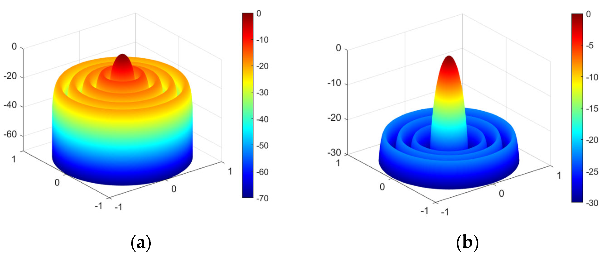
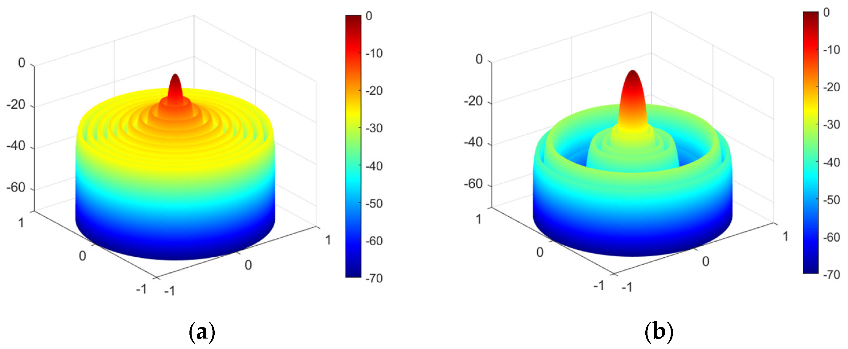
6.5. Simulation Design of Planar Array Antennas

In this final example, a $16\times 16$ planar array antennas was simulated and compared with the GA in Ref. [40]. This GA employed four distinct techniques: Gaussian, Kaiser, Hamming, and Blackman, with the aim of SLL reduction. The planar array antenna has 256 elements optimized, and the mainbeam width was configured as $12°$. The population size of the NCGWO algorithm was set to 64, and the maximum number of iterations was set to 200.

Table 8. Results for planar array antennas.

Algorithm	Peak SLL (dB)	Mainbeam (°)
Gaussian	−22.8200	12
Kaiser	−22.0330	12
Hamming	−22.820	12
Blackman	−32.0070	16
GWO	−27.5697	12
IGWO	−30.5697	12
NCGWO	−34.8303	12

shows the optimization results. The PSLL of the NCGWO algorithm was −34.8303 dB, which was 12.0103 dB, 12.7973 dB, 12.0103 dB, 2.8233 dB, 6.8993 dB, and 4.2606 dB lower than those of the Gaussian, Kaiser, Hamming, Blackman, GWO, and IGWO, respectively. This Blackman method reduces the PSLL below 30 dB, but its main- beam width widens by $4°$. The NCGWO algorithm mitigates the PSLL of the planar array antennas and keeps the beam width unchanged. Figure 17 presents a 3D representation of the planar array and the current amplitude of each array element.

7. Conclusions

The GWO algorithm has been improved in terms of performance, and a new version of the GWO algorithm called the NCGWO algorithm was proposed, where logistic-tent double mapping was adopted to produce a more uniformly distributed initial population. The convergence factor was enhanced to regulate the convergence factor by exponential attenuation of the algorithm and to dynamically stabilize its local and global convergence capabilities.

In this study, the linear and planar array antennas patterns were synthesized using the NCGWO algorithm. The proposed algorithm can suppress the SLL, form deep nulls at multiple design locations, shorten the runtime, and attain better performance.

The NCGWO algorithm has numerous applications, including machine learning, image processing, control engineering, and power systems. In the future, in-depth research should be conducted in these fields to apply the algorithm to more complex and practical problems.

References

1. Balanis, C.A. Antenna Theory and Design; John Wiley & Sons: New York, NY, USA, 1997. [Google Scholar]
2. Cheng, Y.-F.; Ding, X.; Shao, W.; Liao, C. A high-gain sparse phased array with wide-angle scanning performance and low sidelobe levels. IEEE Access 2019, 7, 31151–31158. [Google Scholar] [CrossRef]
3. Douhi, S.; Islam, T.; Saravanan, R.A.; Eddiai, A.; Das, S.; Cherkaoui, O. Design of a Flexible Rectangular Antenna Array with High Gain for RF Energy Harvesting and Wearable Devices. J. Nano Electron. Phys. 2023, 15, 03010. [Google Scholar] [CrossRef]
4. Vescovo, R. Null synthesis by phase control for antenna arrays. Electron. Lett. 2000, 36, 198–199. [Google Scholar] [CrossRef]
5. Das, A.; Mandal, D.; Kar, R. An optimal circular antenna array design considering mutual coupling using heuristic approaches. Int. J. RF Microw. Comput. Eng. 2020, 30, 1–14. [Google Scholar] [CrossRef]
6. Kandregula, V.R.; Lazaridis, P.I.; Zaharis, Z.D.; Ahmed, Q.Z.; Khan, F.A.; Hafeez, M.; Chochliouros, I.P. Simulation Analysis of a Wideband Antenna on a Drone. In Proceedings of the 2022 IEEE International Black Sea Conference on Communications and Networking (BlackSeaCom), Sofia, Bulgaria, 6–9 June 2022; pp. 288–292. [Google Scholar]
7. Sarker, M.A.; Hossain, M.S.; Masud, M.S. Robust beamforming synthesis technique for low side lobe level using taylor excited antenna array. In Proceedings of the 2016 2nd International Conference on Electrical, Computer & Telecommunication Engineering (ICECTE), Rajshahi, Bangladesh, 8–10 December 2016; pp. 1–4. [Google Scholar]
8. Mirjalili, S.; Mirjalili, S.M.; Lewis, A. Grey wolf optimizer. Expert Syst. Appl. 2016, 47, 106–119. [Google Scholar] [CrossRef]
9. Güneş, F.; Tokan, F. Pattern search optimization with applications on synthesis of linear antenna arrays. Expert Syst. Appl. 2010, 37, 4698–4705. [Google Scholar] [CrossRef]
10. Singh, U.; Kamal, T. Design of non-uniform circular antenna arrays using biogeography-based optimisation. IET Microw. Antennas Propag. 2011, 5, 1365–1370. [Google Scholar] [CrossRef]
11. Kaur, K.; Banga, V.K. ‘Optimization of linear antenna array using firefly algorithm. Int. J. Sci. Eng. Res. 2013, 4, 601–606. [Google Scholar]
12. Zhang, Z.; Li, T.; Yuan, F.; Yin, L. Synthesis of Linear Antenna Array Using Genetic Algorithm to Control Side Lobe Level. In Computer Engineering and Networking; Springer: Cham, Switzerland, 2013; pp. 39–46. [Google Scholar]
13. Yang, S.; Gan, Y.B.; Qing, A. Antenna-array pattern nulling using a differential evolution algorithm. Int. J. RF Microw. Comput. Eng. 2003, 14, 57–63. [Google Scholar] [CrossRef]
14. Abdelkader, E.M.; Moselhi, O.; Marzouk, M.; Zayed, T. An exponential chaotic differential evolution algorithm for optimizing bridge maintenance plans. Autom. Constr. 2022, 134, 104107. [Google Scholar] [CrossRef]
15. Saremi, S.; Mirjalili, S.; Lewis, A. Grasshopper optimisation algorithm: Theory and application. Adv. Eng. Softw. 2017, 105, 30–47. [Google Scholar] [CrossRef]
16. Xia, G.; Han, Z.; Zhao, B.; Wang, X. Local path planning for unmanned surface vehicle collision avoidance based on modified quantum particle swarm optimization. Complexity 2020, 2020, 3095426. [Google Scholar] [CrossRef]
17. Al-Azza, A.A.; Al-Jodah, A.A.; Harackiewicz, F.J. Spider monkey optimization: A novel technique for antenna optimization. IEEE Antennas Wirel. Propag. Lett. 2015, 15, 1016–1019. [Google Scholar] [CrossRef]
18. Zervoudakis, K.; Tsafarakis, S. A mayfly optimization algorithm. Comput. Ind. Eng. 2020, 145, 106559. [Google Scholar] [CrossRef]
19. Mahto, S.K.; Choubey, A.; Suman, S. Linear array synthesis with minimum side lobe level and null control using wind driven optimization. In Proceedings of the 2015 International Conference on Signal Processing and Communication Engineering Systems, Guntur, India, 2–3 January 2015; pp. 191–195. [Google Scholar]
20. Guo, H.; Li, J.; Hao, H.; Song, P.; Zhang, L.; Zhang, X. Synthesis of Linear Antenna Array for Wireless Power Transmission. Synthesis 2023, 2023, 6–27. [Google Scholar] [CrossRef]
21. Pavani, T.; Padmavathi, K.; Kumari, C.U.; Ushasree, A. Design of array antennas via atom search optimization. Mater. Today Proc. 2023, 80, 2051–2054. [Google Scholar] [CrossRef]
22. Lakhlef, N.; Oudira, H.; Dumond, C. Failure Correction of Linear Antenna Array using Grey Wolf Optimization. In Proceedings of the 2020 6th IEEE Congress on Information Science and Technology (CiSt), Agadir-Essaouira, Morocco, 5–12 June 2021; pp. 384–388. [Google Scholar]
23. Zhao, K.X.; Liu, Y.; Hu, K. Optimal Pattern Synthesis of Array Antennas Using Improved Grey Wolf Algorithm. In Proceedings of the 2022 IEEE 12th International Conference on Electronics Information and Emergency Communication (ICEIEC), Beijing, China, 15–17 July 2022; pp. 172–175. [Google Scholar]
24. Persohn, K.J.; Povinelli, R.J. Analyzing logistic map pseudorandom number generators for periodicity induced by finite precision floating-point representation. Chaos Solitons Fractals 2012, 45, 238–245. [Google Scholar] [CrossRef]
25. Nezhad, S.Y.D.; Safdarian, N.; Zadeh, S.A.H. New method for fingerprint images encryption using DNA sequence and chaotic tent map. Optik 2020, 224, 165661. [Google Scholar] [CrossRef]
26. Hua, Z.; Zhu, Z.; Yi, S.; Zhang, Z.; Huang, H. Cross-plane colour image encryption using a two-dimensional logistic tent modular map. Inf. Sci. 2021, 546, 1063–1083. [Google Scholar] [CrossRef]
27. Lawnik, M. Combined logistic and tent map. J. Phys. Conf. Ser. 2018, 1141, 012132. [Google Scholar] [CrossRef]
28. Panda, G.; Pradhan, P.M.; Majhi, B. IIR system identification using cat swarm optimization. Expert Syst. Appl. 2011, 38, 12671–12683. [Google Scholar] [CrossRef]
29. Tan, F.; Zhao, J.; Wang, Q. A grey wolf optimization algorithm with improved nonlinear convergence. Microelectron. Comput. 2019, 36, 89–95. [Google Scholar]
30. Li, X.; Luk, K.M. The grey wolf optimizer and its applications in electromagnetics. IEEE Trans. Antennas Propag. 2019, 68, 2186–2197. [Google Scholar] [CrossRef]
31. El-Kenawy, E.-S.M.; Mirjalili, S.; Alassery, F.; Zhang, Y.-D.; Eid, M.M.; El-Mashad, S.Y.; Aloyaydi, B.A.; Ibrahim, A.; Abdelhamid, A.A. Novel meta-heuristic algorithm for feature selection, unconstrained functions and engineering problems. IEEE Access 2022, 10, 40536–40555. [Google Scholar] [CrossRef]
32. Raji, M.F.; Zhao, H.; Monday, H.N. Fast optimization of sparse antenna array using numerical Green’s function and genetic algorithm. Int. J. Numer. Model. Electron. Netw. Devices Fields 2020, 33, e2544. [Google Scholar] [CrossRef]
33. Guo, Q.; Wang, Y.; Li, Y.; Qi, L.; Chernogor, L.F. Pattern synthesis of nonuniform linear antenna array based on FFDM. Digit. Signal Process. 2023, 137, 104022. [Google Scholar] [CrossRef]
34. Boopalan, N.; Ramasamy, A.K.; Nagi, F. A Comparison of Faulty Antenna Detection Methodologies in Planar Array. Appl. Sci. 2023, 13, 3695. [Google Scholar] [CrossRef]
35. Owoola, E.O.; Xia, K.; Wang, T.; Umar, A.; Akindele, R.G. Pattern synthesis of uniform and sparse linear antenna array using mayfly algorithm. IEEE Access 2021, 9, 77954–77975. [Google Scholar] [CrossRef]
36. Wang, H.; Liu, C.; Wu, H.; Li, B.; Xie, X. Optimal pattern synthesis of linear antenna array and broadband design of whip antenna using grasshopper optimization algorithm. Int. J. Antennas Propag. 2020, 2020, 5904018. [Google Scholar] [CrossRef]
37. Khodier, M.M.; Christodoulou, C.G. Linear antenna array geometry synthesis with minimum sidelobe level and null control using particle swarm optimization. IEEE Trans. Antennas Propag. 2005, 53, 2674–2679. [Google Scholar] [CrossRef]
38. Bayraktar, Z.; Komurcu, M.; Bossard, J.A.; Werner, D.H. The wind driven optimization technique and its application in electromagnetics. IEEE Trans. Antennas Propag. 2013, 61, 2745–2757. [Google Scholar] [CrossRef]
39. Pappula, L.; Ghosh, D. Linear antenna array synthesis using cat swarm optimization. AEU Int. J. Electron. Commun. 2014, 68, 540–549. [Google Scholar] [CrossRef]
40. Aboul-Seoud, A.K.; Mahmoud, A.K.; Hafez, A.E.D.S. A sidelobe level reduction (SLL) for planar array antennas with −30 dB attenuators weight precision. Aerosp. Sci. Technol. 2010, 14, 316–320. [Google Scholar] [CrossRef]
Figure 1. Hierarchy of grey wolves.
Electronics 12 04087 g001
Figure 2. Wolves in 2D space.
Electronics 12 04087 g002
Figure 3. Population distribution of chaotic mapping.
Electronics 12 04087 g003
Figure 4. Convergence coefficients.
Electronics 12 04087 g004
Figure 5. Flow chart of the nonlinear chaotic grey wolf optimization (NCGWO) algorithm.
Electronics 12 04087 g005
Figure 6. Illustration of the two-dimensional versions of the test functions. (a,b) are unimodal functions; (c,d) are multimodal functions.
Electronics 12 04087 g006
Figure 7. (a) Uniform LAA geometry; (b) sparse LAA geometry.
Electronics 12 04087 g007
Figure 8. Planar array antennas geometry.
Electronics 12 04087 g008
Figure 9. (a) Radiation patterns of a 10-element linear array antenna SLL; (b) iteration curve.
Electronics 12 04087 g009
Figure 10. 3D radiation patterns of a 10-element linear array antenna SLL near the main lobe minimization: (a) before and (b) after.
Electronics 12 04087 g010
Figure 11. (a) Radiation patterns of the SLL of a 20-element linear array antenna with a lower notch; (b) iteration curve.
Electronics 12 04087 g011
Figure 12. 3D radiation patterns of the SLL of a 20-element linear array antenna with a lower notch: (a) before and (b) after.
Electronics 12 04087 g012
Figure 13. (a) Radiation patterns of the SLL of a 10-element sparse linear array antenna; (b) iteration curve.
Electronics 12 04087 g013
Figure 14. 3D radiation patterns of the SLL of a 10-element sparse linear array antenna: (a) before and (b) after.
Electronics 12 04087 g014
Figure 15. (a) Radiation patterns of the SLL minimization and null of 32-element sparse linear array antennas; (b) iteration curve.
Electronics 12 04087 g015
Figure 16. 3D radiation patterns of the SLL minimization and null of 32-element sparse linear array antennas: (a) before and (b) after.
Electronics 12 04087 g016
Figure 17. 3D radiation patterns of the SLL minimization of planar array antennas: (a) side view and (b) current amplitude of each array element.
Electronics 12 04087 g017