
Collaborative Self-Supervised Transductive Few-Shot Learning for Remote Sensing Scene Classification

Abstract
:1. Introduction
- (1)
- We propose a collaborative self-supervised training strategy for few-shot scene classification. Based on the transfer learning paradigm, our approach allows the model to directly freeze and perform inference after self-supervised training, eliminating the need for complex episode-based training procedures in metric learning.
- (2)
- We introduce the simple soft k-means (SKM) classifier for the few-shot transductive inference. Compared to inductive inference, our model can benefit from more sample references for inference, and it is also simpler compared to the complex graph neural network of transductive inference.
2. Related Works
2.1. Few-Shot Remote Sensing Scene Classification
Self-Supervised Learning
3. Methodology
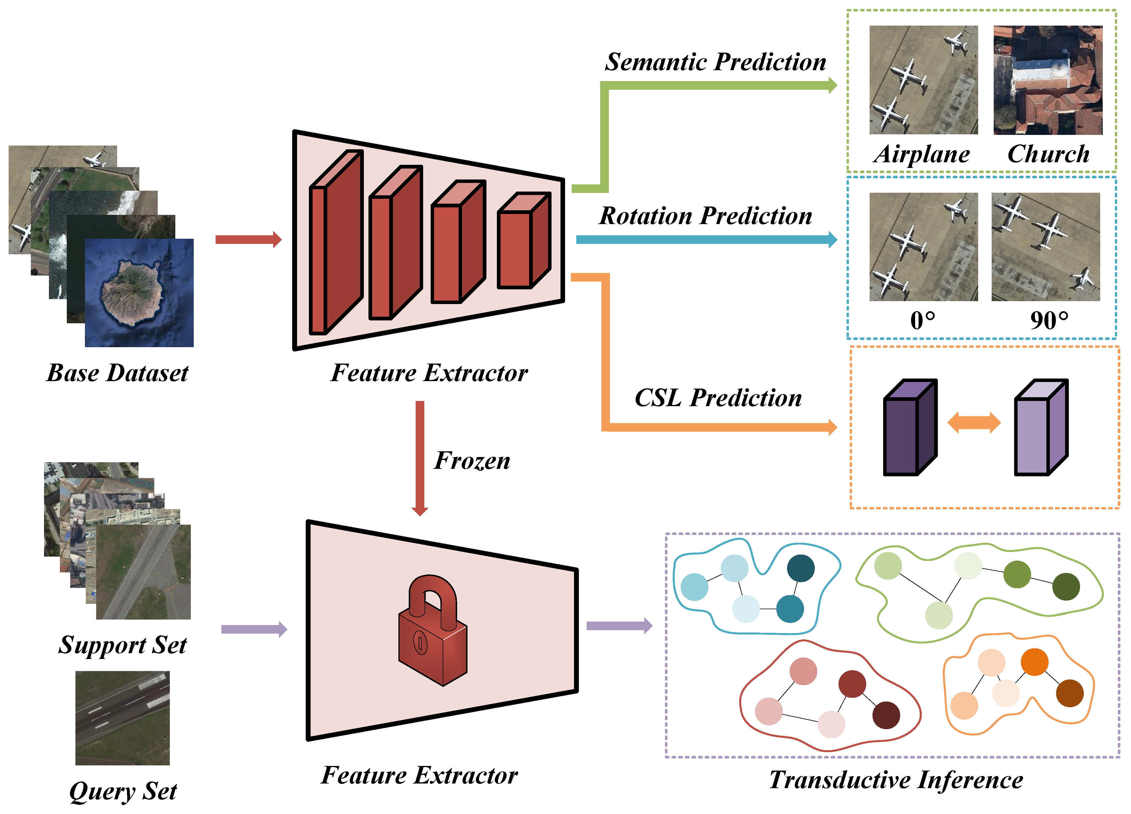
3.1. Overview
3.2. Collaborative Self-Supervised Learning
3.3. Transductive Inference
4. Experimental Results and Analysis
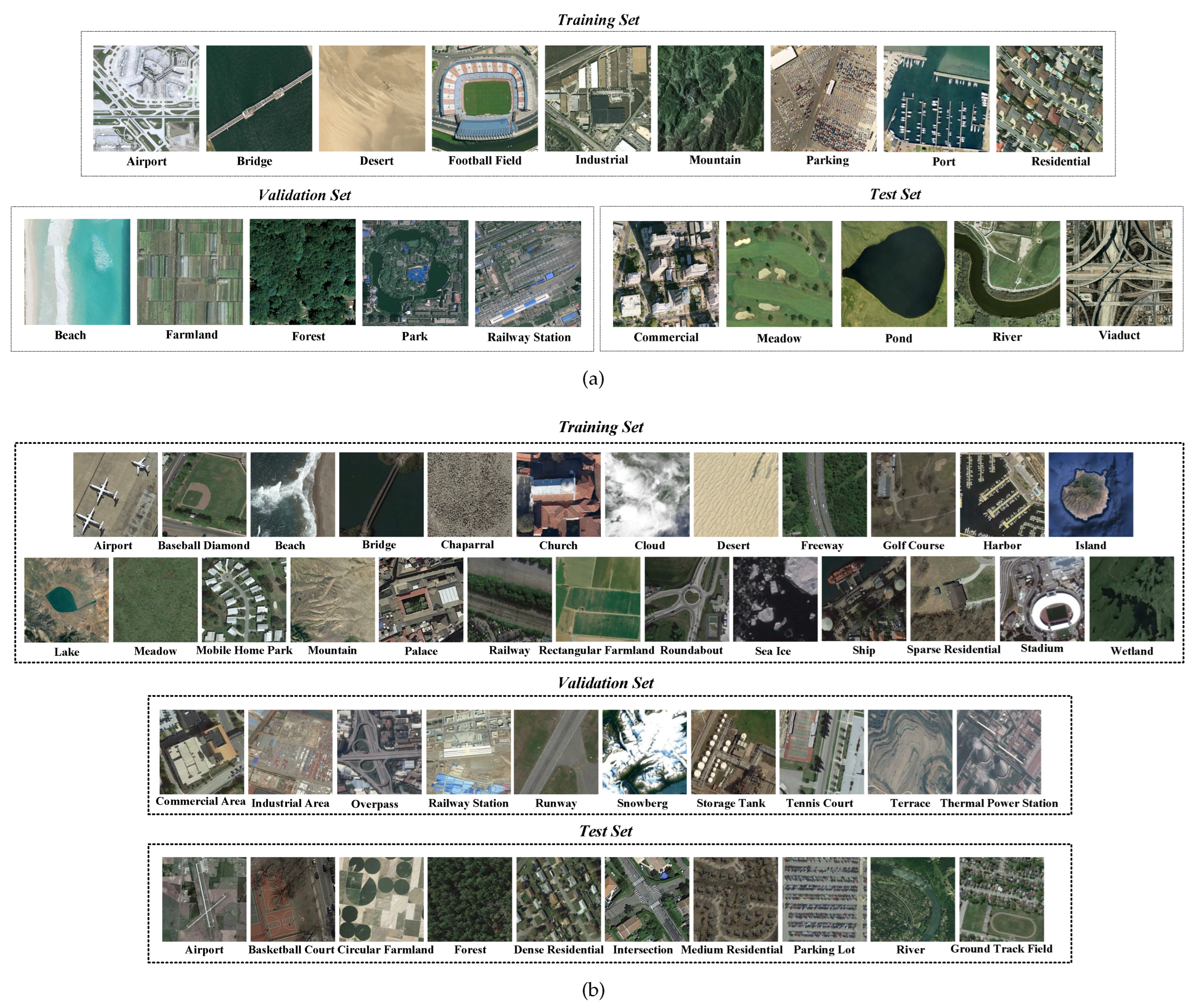
4.1. Datasets
4.2. Implementation Details
4.3. Comparison with Other Methods
4.3.1. Results on the WHU-RS19 Dataset
4.3.2. Results on the NWPU-RESISC45 Dataset
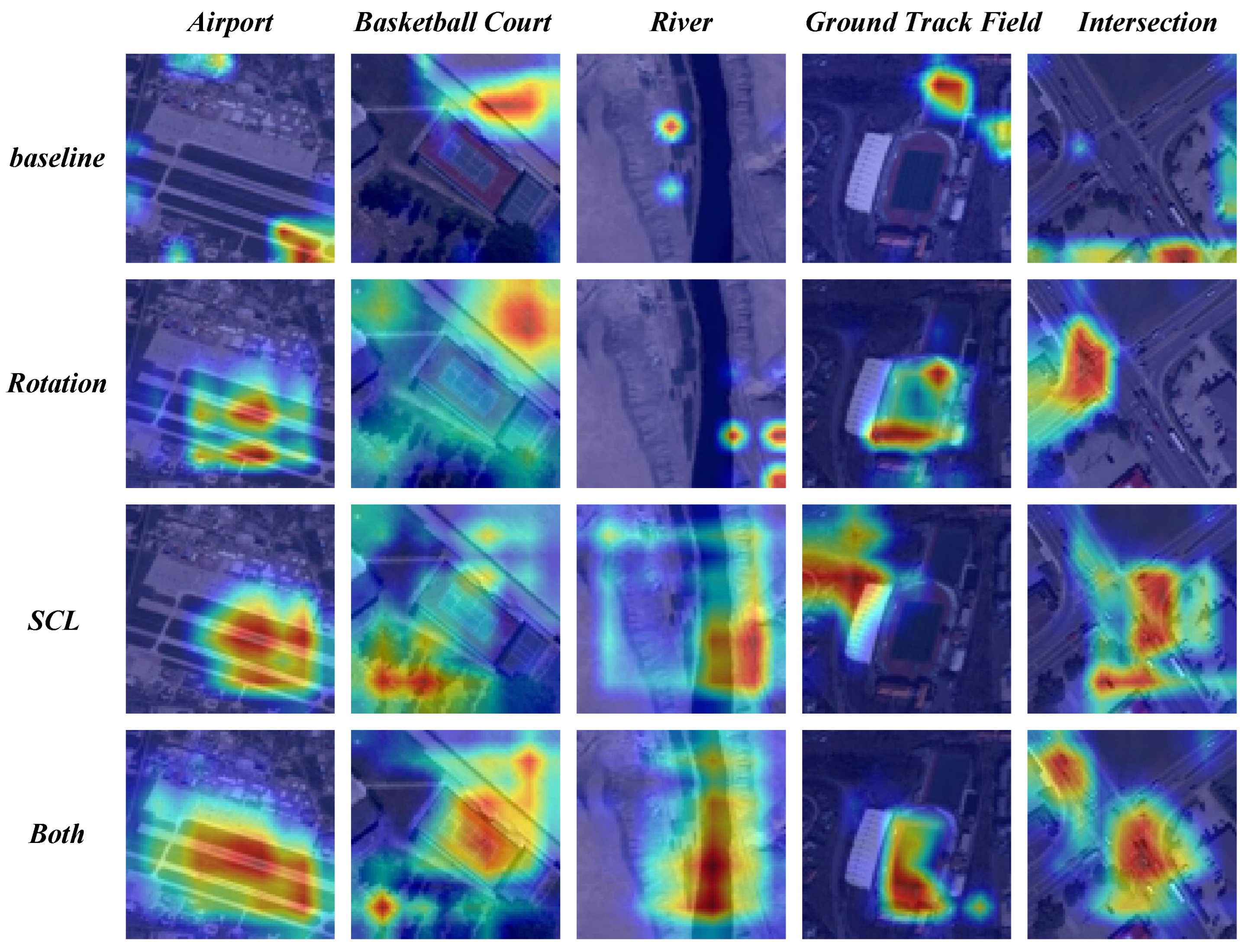
5. Discussion
6. Conclusions
Author Contributions
Funding
Data Availability Statement
Conflicts of Interest
References
- Cheng, G.; Xie, X.; Han, J.; Guo, L.; Xia, G.S. Remote sensing image scene classification meets deep learning: Challenges, methods, benchmarks, and opportunities. IEEE J. Sel. Top. Appl. Earth Obs. Remote Sens. 2020, 13, 3735–3756. [Google Scholar] [CrossRef]
- Zhu, Q.; Guo, X.; Li, Z.; Li, D. A review of multi-class change detection for satellite remote sensing imagery. Geo-Spat. Inf. Sci. 2022, 1–15. [Google Scholar] [CrossRef]
- Wang, Z.; Li, J.; Liu, Y.; Xie, F.; Li, P. An adaptive surrogate-assisted endmember extraction framework based on intelligent optimization algorithms for hyperspectral remote sensing images. Remote Sens. 2022, 14, 892. [Google Scholar] [CrossRef]
- Li, H.; Li, J.; Zhao, Y.; Gong, M.; Zhang, Y.; Liu, T. Cost-sensitive self-paced learning with adaptive regularization for classification of image time series. IEEE J. Sel. Top. Appl. Earth Obs. Remote Sens. 2021, 14, 11713–11727. [Google Scholar] [CrossRef]
- Zhu, Q.; Guo, X.; Deng, W.; Shi, S.; Guan, Q.; Zhong, Y.; Zhang, L.; Li, D. Land-use/land-cover change detection based on a Siamese global learning framework for high spatial resolution remote sensing imagery. ISPRS J. Photogramm. Remote Sens. 2022, 184, 63–78. [Google Scholar] [CrossRef]
- Xia, G.S.; Hu, J.; Hu, F.; Shi, B.; Bai, X.; Zhong, Y.; Zhang, L.; Lu, X. AID: A benchmark data set for performance evaluation of aerial scene classification. IEEE Trans. Geosci. Remote Sens. 2017, 55, 3965–3981. [Google Scholar] [CrossRef]
- Cheng, G.; Han, J.; Guo, L.; Qian, X.; Zhou, P.; Yao, X.; Hu, X. Object detection in remote sensing imagery using a discriminatively trained mixture model. ISPRS J. Photogramm. Remote Sens. 2013, 85, 32–43. [Google Scholar] [CrossRef]
- Wang, Q.; Liu, S.; Chanussot, J.; Li, X. Scene classification with recurrent attention of VHR remote sensing images. IEEE Trans. Geosci. Remote Sens. 2018, 57, 1155–1167. [Google Scholar] [CrossRef]
- Wang, Q.; Gao, J.; Lin, W.; Yuan, Y. Learning from synthetic data for crowd counting in the wild. In Proceedings of the IEEE/CVF Conference on Computer Vision and Pattern Recognition, Long Beach, CA, USA, 15–20 June 2019; pp. 8198–8207. [Google Scholar]
- Zhang, L.; Zhang, L.; Du, B. Deep learning for remote sensing data: A technical tutorial on the state of the art. IEEE Geosci. Remote Sens. Mag. 2016, 4, 22–40. [Google Scholar] [CrossRef]
- Zhang, L.; Zhang, L.; Tao, D.; Huang, X. On combining multiple features for hyperspectral remote sensing image classification. IEEE Trans. Geosci. Remote Sens. 2011, 50, 879–893. [Google Scholar] [CrossRef]
- Qian, X.; Lin, S.; Cheng, G.; Yao, X.; Ren, H.; Wang, W. Object detection in remote sensing images based on improved bounding box regression and multi-level features fusion. Remote Sens. 2020, 12, 143. [Google Scholar] [CrossRef]
- Zhang, Y.; Gong, M.; Zhang, M.; Li, J. Self-Supervised Monocular Depth Estimation With Self-Perceptual Anomaly Handling. IEEE Trans. Neural Netw. Learn. Syst. 2023, 1–15. [Google Scholar] [CrossRef] [PubMed]
- Gong, M.; Zhao, Y.; Li, H.; Qin, A.K.; Xing, L.; Li, J.; Liu, Y.; Liu, Y. Deep Fuzzy Variable C-Means Clustering Incorporated with Curriculum Learning. IEEE Trans. Fuzzy Syst. 2023, 1–15. [Google Scholar] [CrossRef]
- Li, J.; Li, H.; Liu, Y.; Gong, M. Multi-fidelity evolutionary multitasking optimization for hyperspectral endmember extraction. Appl. Soft Comput. 2021, 111, 107713. [Google Scholar] [CrossRef]
- Qian, X.; Zeng, Y.; Wang, W.; Zhang, Q. Co-saliency detection guided by group weakly supervised learning. IEEE Trans. Multimedia 2022, 25, 1810–1818. [Google Scholar] [CrossRef]
- Lang, C.; Cheng, G.; Tu, B.; Han, J. Global Rectification and Decoupled Registration for Few-Shot Segmentation in Remote Sensing Imagery. IEEE Trans. Geosci. Remote. Sens. 2023, 61, 5617211. [Google Scholar] [CrossRef]
- Gao, K.; Liu, B.; Yu, X.; Qin, J.; Zhang, P.; Tan, X. Deep relation network for hyperspectral image few-shot classification. Remote Sens. 2020, 12, 923. [Google Scholar] [CrossRef]
- Zheng, W.; Tian, X.; Yang, B.; Liu, S.; Ding, Y.; Tian, J.; Yin, L. A few shot classification methods based on multiscale relational networks. Appl. Sci. 2022, 12, 4059. [Google Scholar] [CrossRef]
- Lang, C.; Wang, J.; Cheng, G.; Tu, B.; Han, J. Progressive Parsing and Commonality Distillation for Few-shot Remote Sensing Segmentation. IEEE Trans. Geosci. Remote. Sens. 2023, 61, 5613610. [Google Scholar] [CrossRef]
- Shuai, W.; Li, J. Few-shot learning with collateral location coding and single-key global spatial attention for medical image classification. Electronics 2022, 11, 1510. [Google Scholar] [CrossRef]
- Oreshkin, B.; Rodríguez López, P.; Lacoste, A. Tadam: Task dependent adaptive metric for improved few-shot learning. In Proceedings of the NeurIPS 2018, Montreal, QC, Canada, 3–8 December 2018; Volume 31. [Google Scholar]
- Lang, C.; Cheng, G.; Tu, B.; Han, J. Learning what not to segment: A new perspective on few-shot segmentation. In Proceedings of the IEEE/CVF Conference on Computer Vision and Pattern Recognition, New Orleans, LA, USA, 18–24 June 2022; pp. 8057–8067. [Google Scholar]
- Gidaris, S.; Komodakis, N. Dynamic Few-Shot Visual Learning Without Forgetting. In Proceedings of the 2018 IEEE/CVF Conference on Computer Vision and Pattern Recognition, Salt Lake City, UT, USA, 18–23 June 2018; pp. 4367–4375. [Google Scholar] [CrossRef]
- Cheng, G.; Cai, L.; Lang, C.; Yao, X.; Chen, J.; Guo, L.; Han, J. SPNet: Siamese-prototype network for few-shot remote sensing image scene classification. IEEE Trans. Geosci. Remote Sens. 2021, 60, 1–11. [Google Scholar] [CrossRef]
- Ji, H.; Yang, H.; Gao, Z.; Li, C.; Wan, Y.; Cui, J. Few-shot scene classification using auxiliary objectives and transductive inference. IEEE Geosci. Remote Sens. Lett. 2022, 19, 1–5. [Google Scholar] [CrossRef]
- Zhai, M.; Liu, H.; Sun, F. Lifelong learning for scene recognition in remote sensing images. IEEE Geosci. Remote Sens. Lett. 2019, 16, 1472–1476. [Google Scholar] [CrossRef]
- Gong, M.; Li, J.; Zhang, Y.; Wu, Y.; Zhang, M. Two-path aggregation attention network with quad-patch data augmentation for few-shot scene classification. IEEE Trans. Geosci. Remote Sens. 2022, 60, 1–16. [Google Scholar] [CrossRef]
- Li, J.; Gong, M.; Liu, H.; Zhang, Y.; Zhang, M.; Wu, Y. Multiform ensemble self-supervised learning for few-shot remote sensing scene classification. IEEE Trans. Geosci. Remote Sens. 2023, 61, 1–16. [Google Scholar] [CrossRef]
- Bendou, Y.; Hu, Y.; Lafargue, R.; Lioi, G.; Pasdeloup, B.; Pateux, S.; Gripon, V. Easy—Ensemble augmented-shot-y-shaped learning: State-of-the-art few-shot classification with simple components. J. Imaging 2022, 8, 179. [Google Scholar] [CrossRef]
- Schonfeld, E.; Ebrahimi, S.; Sinha, S.; Darrell, T.; Akata, Z. Generalized Zero- and Few-Shot Learning via Aligned Variational Autoencoders. In Proceedings of the 2019 IEEE/CVF Conference on Computer Vision and Pattern Recognition (CVPR), Long Beach, CA, USA, 15–20 June 2019; pp. 8239–8247. [Google Scholar] [CrossRef]
- Ye, H.J.; Hu, H.; Zhan, D.C.; Sha, F. Few-Shot Learning via Embedding Adaptation With Set-to-Set Functions. In Proceedings of the 2020 IEEE/CVF Conference on Computer Vision and Pattern Recognition (CVPR), Seattle, WA, USA, 13–19 June 2020; pp. 8805–8814. [Google Scholar] [CrossRef]
- Chen, W.Y.; Liu, Y.C.; Kira, Z.; Wang, Y.C.F.; Huang, J.B. A closer look at few-shot classification. arXiv 2019, arXiv:1904.04232. [Google Scholar]
- Zhang, Y.; Gong, M.; Li, J.; Feng, K.; Zhang, M. Autonomous perception and adaptive standardization for few-shot learning. Knowl.-Based Syst. 2023, 277, 110746. [Google Scholar] [CrossRef]
- Li, L.; Han, J.; Yao, X.; Cheng, G.; Guo, L. DLA-MatchNet for few-shot remote sensing image scene classification. IEEE Trans. Geosci. Remote Sens. 2020, 59, 7844–7853. [Google Scholar] [CrossRef]
- Zeng, Q.; Geng, J.; Jiang, W.; Huang, K.; Wang, Z. IDLN: Iterative distribution learning network for few-shot remote sensing image scene classification. IEEE Geosci. Remote Sens. Lett. 2021, 19, 1–5. [Google Scholar] [CrossRef]
- Huang, W.; Yuan, Z.; Yang, A.; Tang, C.; Luo, X. TAE-net: Task-adaptive embedding network for few-shot remote sensing scene classification. Remote Sens. 2021, 14, 111. [Google Scholar] [CrossRef]
- Jaiswal, A.; Babu, A.R.; Zadeh, M.Z.; Banerjee, D.; Makedon, F. A survey on contrastive self-supervised learning. Technologies 2020, 9, 2. [Google Scholar] [CrossRef]
- Zhai, X.; Oliver, A.; Kolesnikov, A.; Beyer, L. S4l: Self-supervised semi-supervised learning. In Proceedings of the IEEE/CVF International Conference on Computer Vision, Seoul, Republic of Korea, 27–28 October 2019; pp. 1476–1485. [Google Scholar]
- Liu, X.; Zhang, F.; Hou, Z.; Mian, L.; Wang, Z.; Zhang, J.; Tang, J. Self-supervised learning: Generative or contrastive. IEEE Trans. Knowl. Data Eng. 2021, 35, 857–876. [Google Scholar] [CrossRef]
- Zhang, Y.; Gong, M.; Li, J.; Zhang, M.; Jiang, F.; Zhao, H. Self-supervised monocular depth estimation with multiscale perception. IEEE Trans. Image Process. 2022, 31, 3251–3266. [Google Scholar] [CrossRef]
- Wang, Y.; Albrecht, C.M.; Braham, N.A.A.; Mou, L.; Zhu, X.X. Self-supervised learning in remote sensing: A review. arXiv 2022, arXiv:2206.13188. [Google Scholar] [CrossRef]
- Hong, D.; Gao, L.; Yao, J.; Yokoya, N.; Chanussot, J.; Heiden, U.; Zhang, B. Endmember-guided unmixing network (EGU-Net): A general deep learning framework for self-supervised hyperspectral unmixing. IEEE Trans. Neural Netw. Learn. Syst. 2021, 33, 6518–6531. [Google Scholar] [CrossRef] [PubMed]
- Hu, M.; Wu, C.; Zhang, L. HyperNet: Self-supervised hyperspectral spatial–spectral feature understanding network for hyperspectral change detection. IEEE Trans. Geosci. Remote Sens. 2022, 60, 1–17. [Google Scholar] [CrossRef]
- Wen, Z.; Liu, Z.; Zhang, S.; Pan, Q. Rotation awareness based self-supervised learning for SAR target recognition with limited training samples. IEEE Trans. Image Process. 2021, 30, 7266–7279. [Google Scholar] [CrossRef]
- Yue, J.; Fang, L.; Rahmani, H.; Ghamisi, P. Self-supervised learning with adaptive distillation for hyperspectral image classification. IEEE Trans. Geosci. Remote Sens. 2021, 60, 1–13. [Google Scholar] [CrossRef]
- Li, X.; Shi, D.; Diao, X.; Xu, H. SCL-MLNet: Boosting few-shot remote sensing scene classification via self-supervised contrastive learning. IEEE Trans. Geosci. Remote Sens. 2021, 60, 1–12. [Google Scholar] [CrossRef]
- Grill, J.B.; Strub, F.; Altché, F.; Tallec, C.; Richemond, P.; Buchatskaya, E.; Doersch, C.; Avila Pires, B.; Guo, Z.; Gheshlaghi Azar, M.; et al. Bootstrap your own latent-a new approach to self-supervised learning. Adv. Neural Inf. Process. Syst. 2020, 33, 21271–21284. [Google Scholar]
- Chen, T.; Kornblith, S.; Norouzi, M.; Hinton, G. A simple framework for contrastive learning of visual representations. In Proceedings of the International Conference on Machine Learning (PMLR), Virtual Event, 13–18 July 2020; pp. 1597–1607. [Google Scholar]
- Li, Y.; Shao, Z.; Huang, X.; Cai, B.; Peng, S. Meta-FSEO: A meta-learning fast adaptation with self-supervised embedding optimization for few-shot remote sensing scene classification. Remote Sens. 2021, 13, 2776. [Google Scholar] [CrossRef]
- Ouali, Y.; Hudelot, C.; Tami, M. Spatial contrastive learning for few-shot classification. In Proceedings of the European Conference on Machine Learning and Knowledge Discovery in Databases (ECML PKDD 2021), Bilbao, Spain, 13–17 September 2021; pp. 671–686. [Google Scholar]
- Sheng, G.; Yang, W.; Xu, T.; Sun, H. High-resolution satellite scene classification using a sparse coding based multiple feature combination. Int. J. Remote Sens. 2012, 33, 2395–2412. [Google Scholar] [CrossRef]
- Cheng, G.; Han, J.; Lu, X. Remote sensing image scene classification: Benchmark and state of the art. Proc. IEEE 2017, 105, 1865–1883. [Google Scholar] [CrossRef]
- Finn, C.; Abbeel, P.; Levine, S. Model-agnostic meta-learning for fast adaptation of deep networks. In Proceedings of the International conference on machine learning (PMLR), Sydney, Australia, 6–11 August 2017; pp. 1126–1135. [Google Scholar]
- Mangla, P.; Kumari, N.; Sinha, A.; Singh, M.; Krishnamurthy, B.; Balasubramanian, V.N. Charting the right manifold: Manifold mixup for few-shot learning. In Proceedings of the 2020 IEEE/CVF Conference on Computer Vision and Pattern Recognition (CVPR), Seattle, WA, USA, 13–19 June 2020; pp. 2218–2227. [Google Scholar]
- Li, Z.; Zhou, F.; Chen, F.; Li, H. Meta-sgd: Learning to learn quickly for few-shot learning. arXiv 2017, arXiv:1707.09835. [Google Scholar]
- Vinyals, O.; Blundell, C.; Lillicrap, T.; Wierstra, D. Matching networks for one shot learning. In Proceedings of the 30th Conference on Neural Information Processing Systems (NIPS 2016), Barcelona, Spain, 5–10 December 2016; Volume 29. [Google Scholar]
- Snell, J.; Swersky, K.; Zemel, R. Prototypical networks for few-shot learning. In Proceedings of the 31st Conference on Neural Information Processing Systems (NIPS 2017), Long Beach, CA, USA, 4–9 December 2017; Volume 30. [Google Scholar]
- Sung, F.; Yang, Y.; Zhang, L.; Xiang, T.; Torr, P.H.; Hospedales, T.M. Learning to compare: Relation network for few-shot learning. In Proceedings of the IEEE Conference on Computer Vision and Pattern Recognition, Salt Lake City, UT, USA, 18–23 June 2018; pp. 1199–1208. [Google Scholar]
- Hou, R.; Chang, H.; Ma, B.; Shan, S.; Chen, X. Cross attention network for few-shot classification. In Proceedings of the 33rd Conference on Neural Information Processing Systems (NeurIPS 2019), Vancouver, BC, Canada, 8–14 December 2019; Volume 32. [Google Scholar]

| Method | 5-Way | |
|---|---|---|
| 1-Shot | 5-Shot | |
| MAML [54] | ||
| LLSR [27] | ||
| Ji et al. [26] | ||
| baseline [33] | ||
| S2M2 [55] | ||
| Meta-SGD [56] | ||
| MatchingNet [57] | ||
| ProtoNet [58] | ||
| RelationNet [59] | ||
| DLA-MatchNet [35] | ||
| IDLN [36] | ||
| TAE-Net [37] | ||
| CAN+T [60] | ||
| SPNet [25] | ||
| DANet [28] | ||
| CSTFSL (Ours) | ||
| Dataset | Method | 5-Way | |
|---|---|---|---|
| 1-Shot | 5-Shot | ||
| WHU-RS19 | baseline | ||
| +Rotation | |||
| +SCL | |||
| CSTFSL | |||
| baseline | |||
| +Rotation | |||
| +SCL | |||
| CSTFSL | |||
| NWPU-RESISC45 | baseline | ||
| +Rotation | |||
| +SCL | |||
| CSTFSL | |||
| baseline | |||
| +Rotation | |||
| +SCL | |||
| CSTFSL | |||
Disclaimer/Publisher’s Note: The statements, opinions and data contained in all publications are solely those of the individual author(s) and contributor(s) and not of MDPI and/or the editor(s). MDPI and/or the editor(s) disclaim responsibility for any injury to people or property resulting from any ideas, methods, instructions or products referred to in the content. |
© 2023 by the authors. Licensee MDPI, Basel, Switzerland. This article is an open access article distributed under the terms and conditions of the Creative Commons Attribution (CC BY) license (https://creativecommons.org/licenses/by/4.0/).
Share and Cite
Han, H.; Huang, Y.; Wang, Z. Collaborative Self-Supervised Transductive Few-Shot Learning for Remote Sensing Scene Classification. Electronics 2023, 12, 3846. https://doi.org/10.3390/electronics12183846
Han H, Huang Y, Wang Z. Collaborative Self-Supervised Transductive Few-Shot Learning for Remote Sensing Scene Classification. Electronics. 2023; 12(18):3846. https://doi.org/10.3390/electronics12183846
Chicago/Turabian StyleHan, Haiyan, Yangchao Huang, and Zhe Wang. 2023. "Collaborative Self-Supervised Transductive Few-Shot Learning for Remote Sensing Scene Classification" Electronics 12, no. 18: 3846. https://doi.org/10.3390/electronics12183846
APA StyleHan, H., Huang, Y., & Wang, Z. (2023). Collaborative Self-Supervised Transductive Few-Shot Learning for Remote Sensing Scene Classification. Electronics, 12(18), 3846. https://doi.org/10.3390/electronics12183846