1. Introduction
The use of energy is a important topic of interest in the field of ground vehicles (GVs) [
1]. GVs such as exploration robots and space probes mostly operate in the complex off-road terrain environment (2.5D environment), and energy consumption can become a problem that restricts their working range and time. So far, scholars have studied battery technology [
2], motor control technology [
3], and gas engine technology [
4] in order to improve energy efficiency.
In this paper, an energy-saving method from the perspective of path planning for GVs is studied. A GV going uphill always consumes a lot of energy to overcome its gravity, which means a path with less up-slope but a bit longer may save more energy than that of the shortest path, which covers many up-slopes. Hence, there will always be some energy-saving paths on the 2.5D map. Meanwhile, some of these paths with longer distances may significantly increase the traveling time, which is also unacceptable. Overall, this yields a multi-objective path planning problem: to find paths on a terrain environment with a good trade-off between energy consumption and distance.
The traditional methods such as violent search [
5], heuristic-based search [
6] and probabilistic search [
7], etc., can solve this multi-objective path planning problem to some extent. However, all of them encounter some shortcomings on this task. The violent search methods have to search a large area with low efficiency. The heuristic-based methods suffer the difficulty of modeling the heuristic function for 2.5D path planning (it is hard to estimate the cost of a path on the terrain map). The probabilistic search methods show unstable performance in the off-road environment.
Lately, deep reinforcement learning (DRL) has emerged as a highly promising approach for tackling path planning problems [
8]. Therefore, in this paper, we employ DRL to establish a multi-objective 2.5D path planning method (DMOP) that focuses on improving planning efficiency while ensuring a good balance between energy consumption and the distance of the planned path. The contribution of this work is listed as below:
Novel topic: A deep reinforcement learning-based multi-objective 2.5D path planning method (DMOP) is proposed for GVs, realizing a good trade-off on distance and energy consumption on off-road terrain environments.
Useful findings: (1) The DMOP plans paths with significant high efficiency in comparison with other methods. (2) The DMOP has powerful reasoning capability that enables it to perform arbitrary untrained planning tasks.
Solved two technical problems: (1) The convergence problem of DQN in high state space is solved by using a hybrid exploration strategy and reward-shaping theory. (2) To tackle the multi-objective 2.5D path planning problem using DRL, an exquisite reward function is designed, incorporating terrain, distance, and border information for modeling.
The remainder of this paper is structured as follows:
Section 2 provides a review of the current research status on 2.5D path planning algorithms. The preliminaries of the 2.5D path planning task are given in
Section 3. Then, the detailed description of the DMOP is introduced in
Section 4.
Section 5 describes the experiments conducted to verify the effectiveness of DMOP and exhibits and analyzes the experimental results. Finally,
Section 6 summarizes this paper and outlines future research directions.
2. Related Works
Path planning methods that consider slope (on 2.5D map) have been studied for years, and researchers are concentrating on finding suitable paths for GVs in complex terrain environments [
9,
10,
11]. In early research, most studies focused on single-object optimization problems, such as traversability or avoiding obstacles. Therefore, scholars are concerned about vehicle dynamics to ensure motion stability [
7,
12,
13]. For instance, a probabilistic road map (PRM)-based path planning method considering traversability is proposed for extreme-terrain rappelling rovers [
7]. Linhui et al. [
12] present an obstacle avoidance path-planning algorithm based on a stereo vision system for intelligent vehicles; such an algorithm uses stereo matching techniques to recognize obstacles. Shin et al. [
13] propose a path planning method for autonomous ground vehicles (AGVs) operating in rough terrain dynamic environments, employing a passivity-based model predictive control. Obviously, these planning methods place less emphasis on the global nature of the path.
As research on 2.5D path planning deepens, scholars are prone to create multi-objective path planning methods that take complex characteristics of 2.5D terrain into account, especially the issues of operational efficiency, energy consumption, and the difficulty of mechanical operation. These works aim to find paths that are energy efficient and easy to pass [
14,
15]. Ma et al. [
16] propose an energy-efficient path planning method built upon an enhanced A* algorithm and a particle swarm algorithm for ground robots in complex outdoor scenarios. This method considers the slope parameter and friction coefficient, which can effectively assist ground robots in traversing areas with various terrain features and landcover types. Based on the hybrid A* method, Ganganath et al. [
17] present a algorithm by incorporating a heuristic energy-cost function, which enables the robots to find energy-efficient paths in steep terrains. Even though A*-based methods are likely to find the optimal or near-optimal path, their performance in terms of search time tends to be poor due to the search mechanism. Moreover, Jiang et al. [
18] investigate a reliable and robust rapidly exploring random tree (R2-RRT*) algorithm for the multi-objective planning mission of AGVs under uncertain terrain environment. However, this kind of method has an unavoidable weaknesses, local minimum, which means it cannot guarantee the quality of the path. Despite the fact that existing research has made notable achievements, the 2.5D path planning method considering energy consumption and the distance of the global path has not been widely studied.
Regarding this topic, our team has previously proposed a heuristic-based method (H3DM) [
19]. In this method, a novel weight decay model is introduced to solve the modeling problem of the heuristic function, and then the path planning with a better trade-off of distance and energy consumption is realized. Nonetheless, the solutions obtained by this method are not good enough regarding the path’s global nature and the search efficiency. Thus, the multi-objective path planning method, which considers the path’s global nature and time efficiency, should be further researched.
With the merit of solving complex programming problems, DRL has achieved much success in Go [
20], video games [
21], internet recommendation systems [
22], etc. Scholars have also proved that DRL has the potential to solve N-P hard problems [
23], such as the traveling salesman problem (TSP) [
24] and the postman problem [
25]. Since the path planning problem is also a kind of N-P hard problem [
26,
27], researchers have begun to apply DRL theory to solve path planning problems. Ren et al. [
28] create a two-stage DRL method, which enables the mobile robot to navigate from any initial point in the continuous workspace to a specific goal location along an optimal path. Based on the double deep Q network, Chu et al. [
29] propose a path planning method for autonomous underwater vehicles under unknown environments with disturbances from ocean currents. These methods have powerful reasoning capabilities and show the great potential of DRL in the field of path planning.
In order to develop a computationally efficient method with a better trade-off of distance and energy consumption, we present the DMOP method using the DRL theory in this paper. The DMOP is composed of a deep Q network (DQN), which can finish the planning task with higher efficiency in comparison with other methods.
4. Dqn-Based Multi-Objective 2.5D Path Planning
In this section, we first present the problem statement, followed by the design of DQN, including the structure of the convolutional neural network (CNN), the modeling of the reward function, and the training strategy, as well as the path-enhanced method. The DMOP method built from these components ultimately solves the multi-objectives 2.5D path planning problem.
4.1. Problem Statement
Though the DQN has the great potential to solve the path planning problem, two technical problems should be solved here: (1) the convergence problem of DQN in high state space; (2) the multi-objective path planning problem.
The convergence problem of DQN in high state space presents a challenge. The construction of the 2.5D map at a relatively high resolution results in a large map size, further exacerbating the issue as the DQN struggles to converge due to the extensive state space. Even for a size of 20*20, the DQN may fail to converge sometimes.
The multi-objective path planning problem involves the goal of finding not only a path from a given start point to a target but also a globally optimal path with a short length and low energy consumption.
4.2. Background and Structure of DQN
DQN is a reinforcement learning technique that combines deep neural networks with Q-learning to tackle complex decision-making tasks [
21]. It leverages deep neural networks to estimate the Q-values of different actions in various states [
30].
As shown in
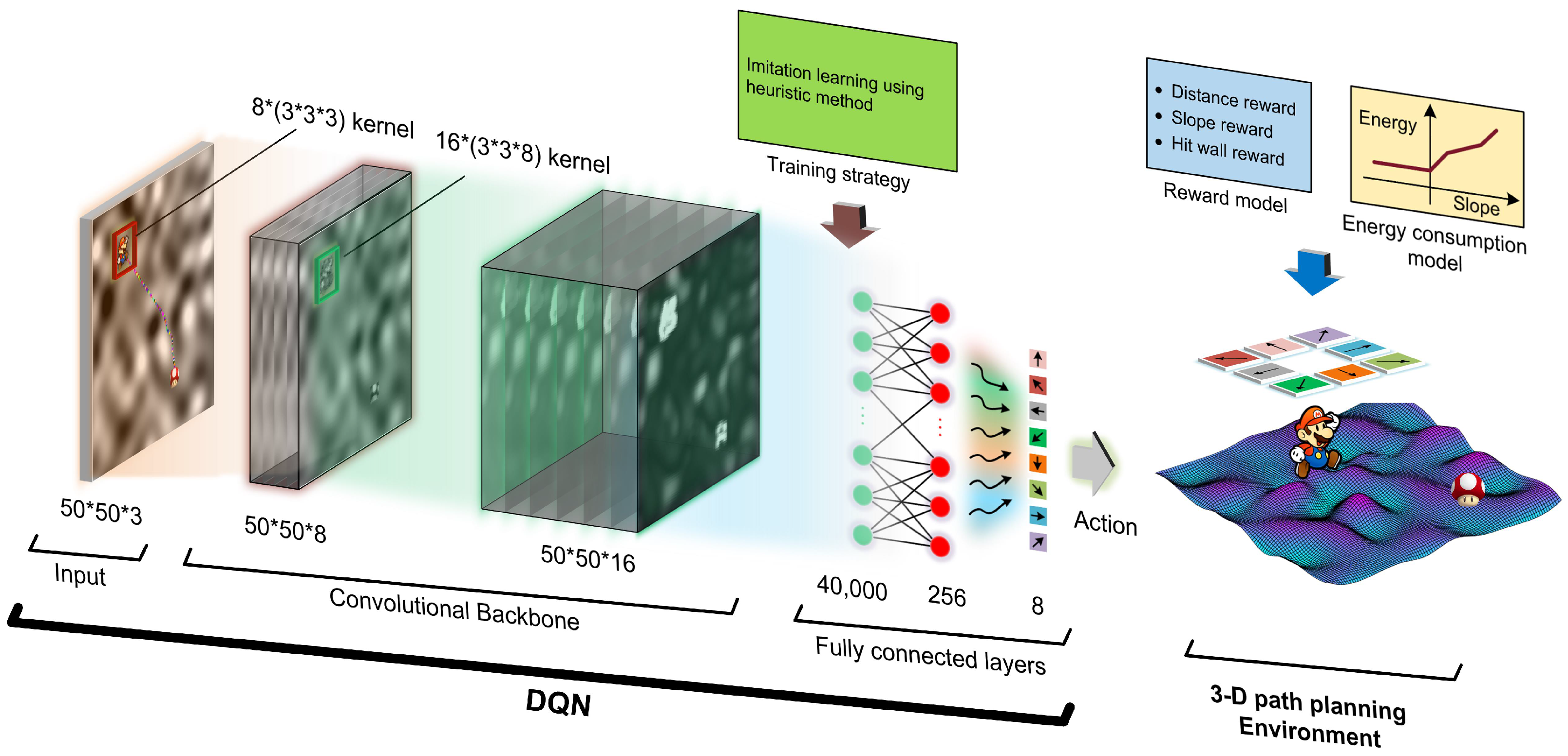
Figure 1, the adopted DQN is a convolutional neural network that is composed of three parts: the input layer, the convolutional backbone, and the fully connected layers.
The input layer is the observation state of the DQN, while the state is a 50*50*3 image (transforming the 100*100*3 map into a 50*50*3 image using the pixel skipping technique) in which Mario, mushroom, and the 2.5D map are drawn on the different channels, respectively.
The convolutional backbone is built with 2 convolutional layers: the size of the convolutional kernel for the first layer is 8*(3*3*3), and the second is 16*(3*3*8). The activation function is ReLu. It should be mentioned that Mario and mushroom are used to replace the single pixel of the current and target point, to allow the network to more easily recognize the current location of agent and target, thus accelerating the learning process. In addition, no pooling layers are used here. According to numerous experiments, using the pooling layer in this structure can lead to a severe convergence problem. The reason may be that too much information is lost after the pooling process.
The fully connected layers consist of three layers. The first layer connects to the output of the last convolutional layer. The second one has 256 nodes; both this layer and the former layer also use ReLu as the activation function. The last layer has 8 nodes that represent the Q value of actions, and it takes a linear function as the activation function.
4.3. Design of Reward Function
The reward function plays a key role in training the DQN. When the size of the map becomes bigger and bigger, the DQN will be more difficult to converge. If the agent only gets the reward at the target, the DQN will hardly converge through random exploration, let alone realize the multi-objective planning. To solve this problem, an exquisite reward function is designed for the 2.5D multi-objective path planning task. Based on the reward-shaping theory [
21], this function is built from the following points:
The DQN aims to find a policy that maximizes the discounted accumulated reward (score), and the goal of this game is to find a path with a good trade-off between distance and energy consumption; hence, the reward for Mario’s step should be negative (penalty), otherwise the DQN will tend to plan a path that maximizes the reward, even if it means making the path as long as possible.
To guide Mario to find the mushroom, a suitable distance-based reward should be provided. In addition, the agent can receive a bigger reward as it gets closer to the target.
Considering the energy consumption in path planning, a slope-based penalty should be given.
To prevent the agent from cheating to obtain a higher score by hitting the wall, the hit-wall penalty should be relatively strong.
A relatively big reward should be given to encourage the agent to remember the experience when reaching the target.
Based on the above ideas, the reward function is modeled as:
where
is the distance penalty,
is the slope penalty,
denotes the hit-wall penalty, and
stands for the reached reward.
4.3.1. Distance Penalty Model
The model of the distance penalty includes two parts:
where
is a global distance penalty, and
is a step distance penalty that is modeled as:
where
is a step distance in 2.5D aspect,
is a factor of the intensity, and
according to a bunch of tests.
alone is not enough as it neglects the terrain information, so the second part
is introduced to compensate for the penalty.
heuristically penalizes the action that leads the next current position too far away from the destination in the 2D aspect. It is modeled as:
where
means the 2D distance between the next current position and the destination, and
is an intensive factor (its value is set according to the size of the map). Here,
.
4.3.2. Slope Penalty Model
The slope penalty can be calculated based on Equation (3). Here, the slope penalty is defined as:
where
k is the intensity factor.
k is set as 5 according to many training experiment. It is easy to understand that the penalty is proportional to energy consumption.
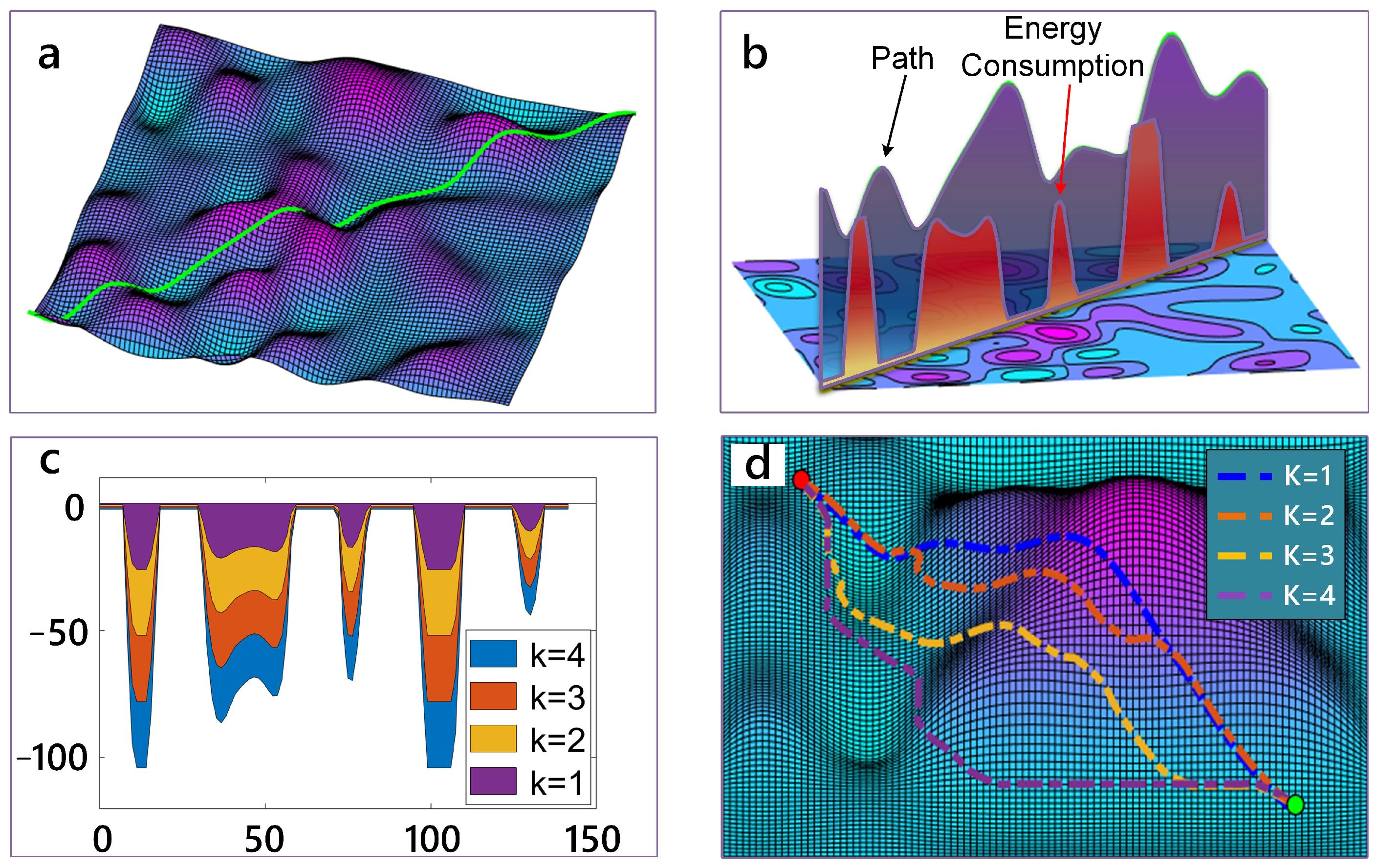
Here, a case is given to illustrate the slope penalty term. For a path depicted in
Figure 2a, the up-slope motion consumes lots of energy (see
Figure 2b). Moreover, we can control the intensity of the slope penalty with a different factor
k (see
Figure 2c). From
Figure 2d, we can see that when
k becomes bigger, the planned path is more sensitive to the slope and tries to avoid going up-slope. Ultimately, we choose
k = 5 as it produces a balanced trade-off between energy consumption and distance in the planned paths.
4.3.3. Hit-Wall Penalty Model
The wall penalty term
is used to prevent the agent from hitting the boundary of the maps for the higher reward and thus from cheating in game.
is modeled as:
where
b is the upper bound, and
. This parameter is set to prevent excessive penalties when the agent is positioned in the four corners of the map, namely, the top-left, bottom-left, top-right, and bottom-right corners.
and
are corresponding penalties to the
x and
y axes, respectively.
denotes the penalty intensity, and
.
and
are defined in a similar way:
where
and
are the specific lines that trigger the wall penalty, and
.
and
are the corresponding coordinates on the XOY plate.
4.3.4. Reached Reward Model
The reached reward
is used to encourage the agent to remember the experiences it has encountered.
where
k is the same factor used in Equation (18). The coefficient “5” is tuned manually according to the training results.
4.4. Hybrid Exploration Strategy
Since the state space is too big, the DQN is difficult to converge through random exploration, even when a well-designed reward function is used. Here, a hybrid exploration strategy is applied to improve the training performance. We design a hybrid exploration strategy that uses the heuristic method to generate useful experience for training the DQN.
The traditional training strategy for DQN initially involves selecting actions with a certain probability, either through random exploration or using DQN’s output, to guide the agent to successfully reach the target and gain valuable experiences for learning. However, in complex 2.5D path planning tasks, this method can lead to difficulties in reaching the target during the exploration process, resulting in a lack of successful experiences to learn from. To obtain more successful experiences and improve the learning efficiency, the exploration strategy has transitioned from pure random exploration to a blend of heuristic methods and random exploration. The heuristic method involves comparing the distances between each neighboring point and the target, with the action corresponding to the minimum distance being selected as the recommended action. In the early stages of training, there is a 60% probability of employing a hybrid exploration strategy, where 50% probability is assigned to selecting random actions and 10% probability is assigned to selecting heuristic actions. The remaining 40% probability is devoted to using actions generated by the DQN (see
Figure 3). As the training goes further, the exploration probability will decrease to a relatively small value (the figure 60% will decrease to 1%, and 40% will increase to 99% at the end). Eventually, the agent acquires the knowledge of how to plan paths.
4.5. Path-Enhanced Method
The planned path on a lower resolution map includes many straight segments that should be curves on the higher resolution map; these segments can be recovered. Here, a path-enhancing method is proposed to transform a lower resolution path (50*50) into a higher one (100*100, or even higher).
The proposed method includes three steps: (1) map the planned path into the corresponding high resolution map, (2) extract the tuning points using the slope information of the path, and (3) connect the extracted points using the cubic spline interpolation method.
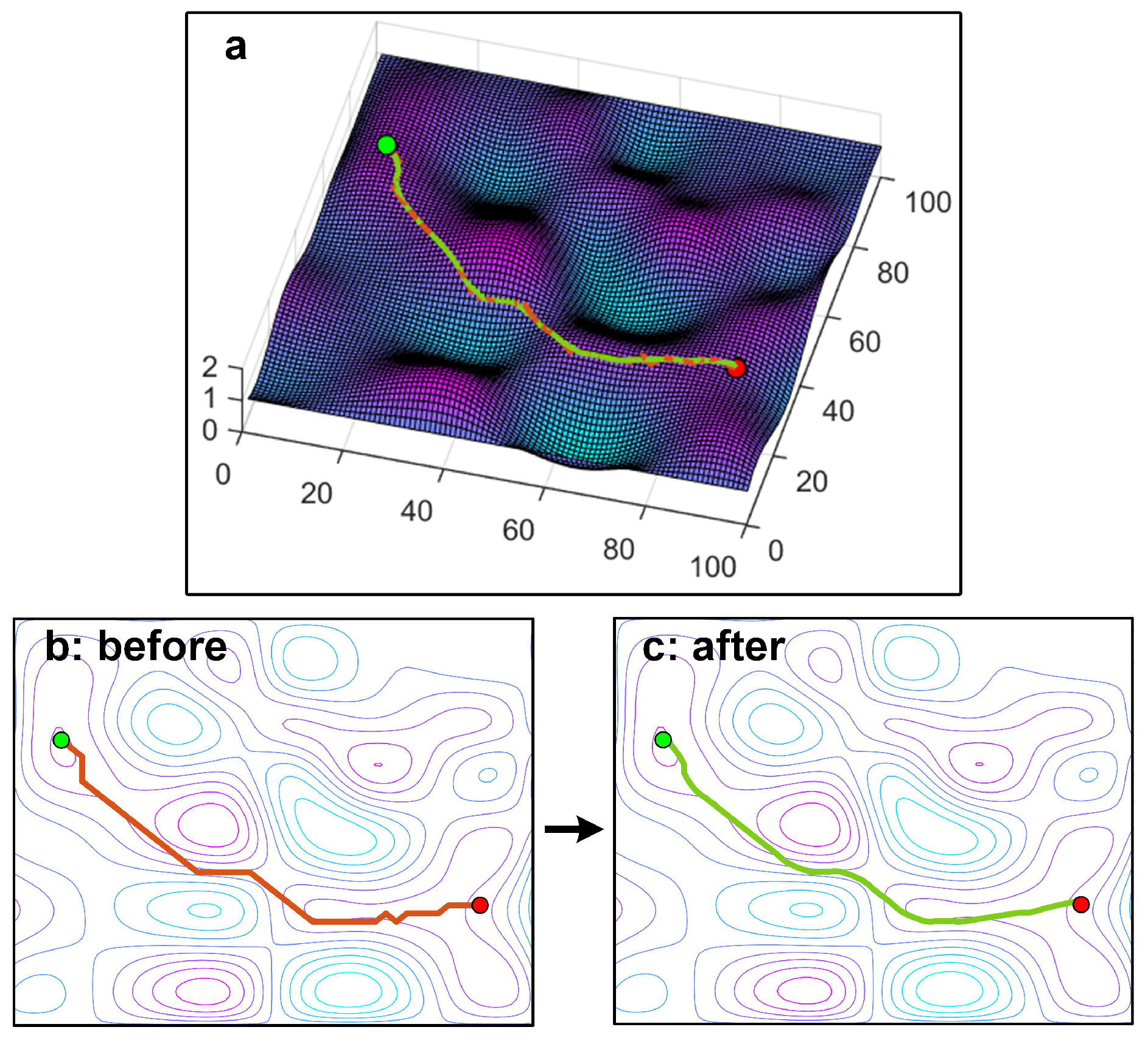
Figure 4 shows an example of a smooth process using the path-enhanced method. It shows that the green curve becomes smoother than the red curve.
4.6. Hyperparameters Setting and Training Result
The DMOP method is trained with multitask, which means that the start point and the target are set randomly in different episodes. The hyperparameters are listed in
Table 1.
In
Figure 5, the curves of reward in many cases are depicted. This result reveals that the convergence problem of DQN with high state space [
21] can be solved via our method. When the DQN is converged, it learns how to recognize Mario and mushroom. In addition, we found an interesting phenomenon: that the bottom of valleys (see the yellow circuits in
Figure 5b) is regarded as the peak by DQN, which means the agent takes as much energy to cross a valley as it does to cross a mountain.
5. Simulation and Analysis
5.1. Setting and Results
The 2.5D map used in this section is set as: both of its x and y axes range in [1, 100], and its z-axis ranges in [0, 2]. This map can be regarded as it is zoomed from a 10 km * 10 km area with a maximum altitude of 200 m. Furthermore, the proposed method is compared with the H3DM method [
19], an improved RRT method [
31], the Dijkstra method [
32], and the
method [
33]. H3DM is a purely heuristic-based algorithm; at its core, it adds a distance weight decay model to the heuristic function to estimate energy consumption and distance. Based on the idea of H3DM, we apply the identical heuristic function model to the A* algorithm. The A* algorithm used in the 2.5D scenario employs a search mechanism the same as that in the 2D case. It evaluates and sorts nodes in the map based on the total cost function, selecting the node with the lowest cost to expand the search path. Dijkstra utilizes the same search mechanism as A*, with the only difference being that it lacks a heuristic function in its total cost function. As for the RRT algorithm, its search strategy is similar to that in 2D, and we enhance the guidance towards the target direction [
34]. After planning the path, we calculate energy consumption data. All these methods are planning for multi-objective, where the energy consumption and path distance are using the same weights in comparison. All the methods run on a computer with NVIDIA GTX 3060 GPU, AMD Ryzen 5600 CPU, and 16G RAM, and the codes are implemented with python. It should be mentioned that the DQN in the DMOP method is trained with multitask, and the tested tasks have not all been used in the training process.
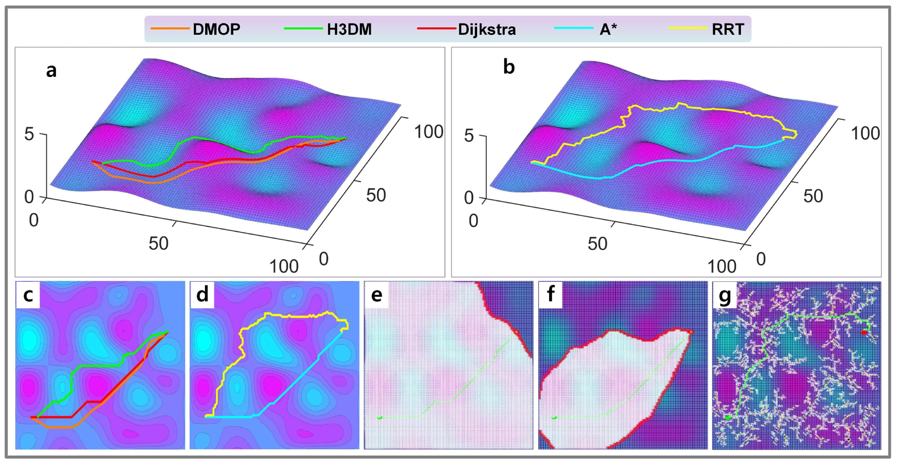
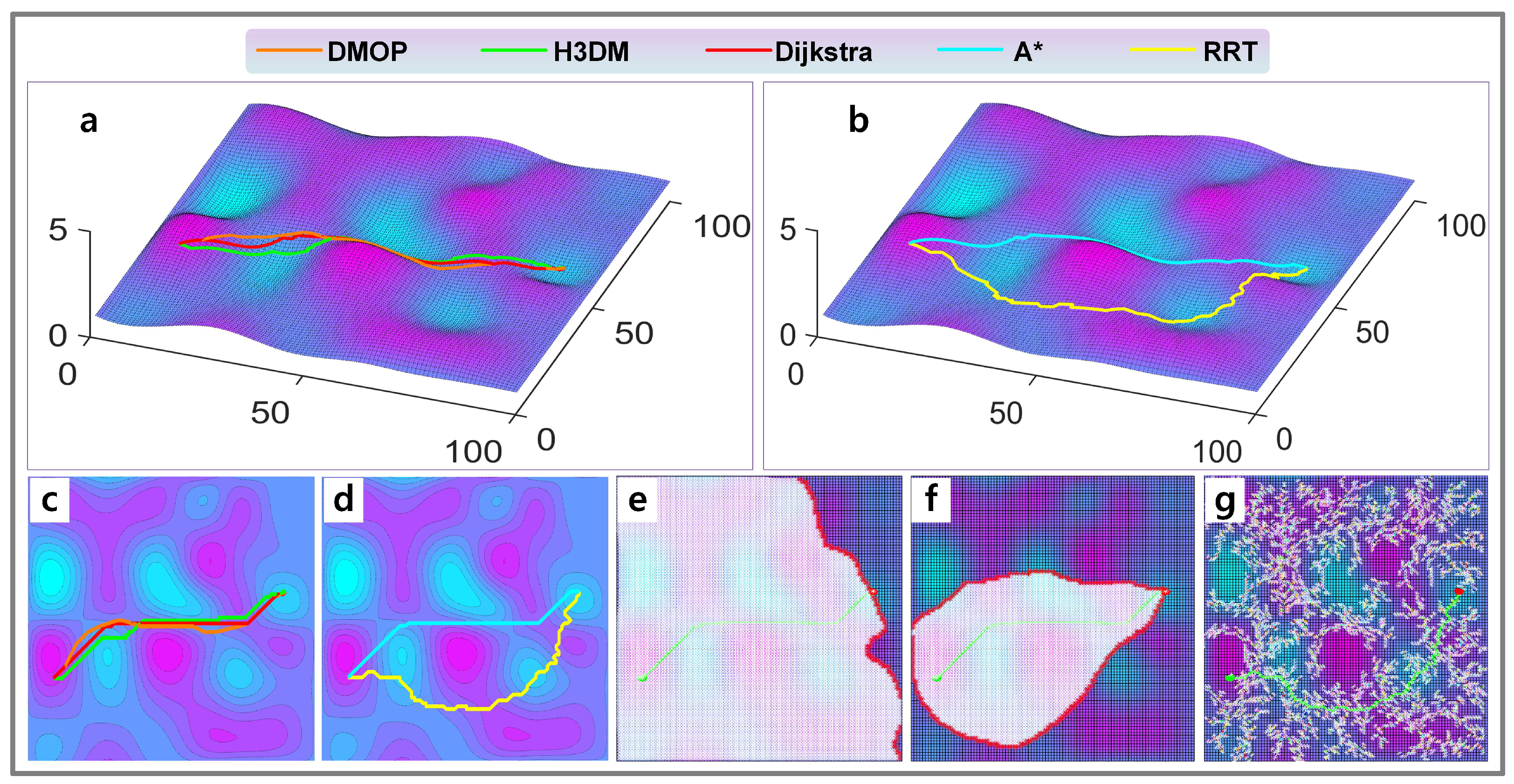
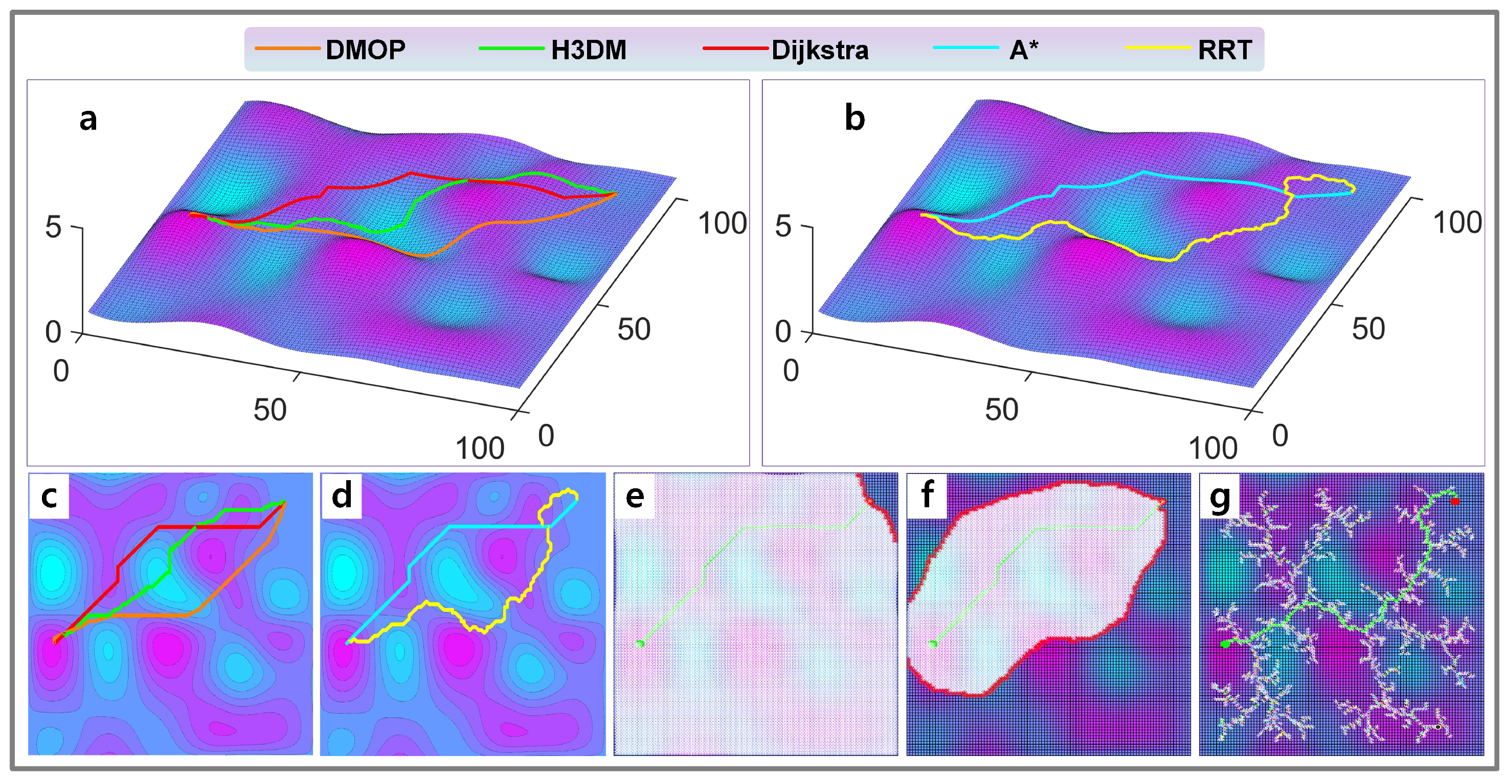
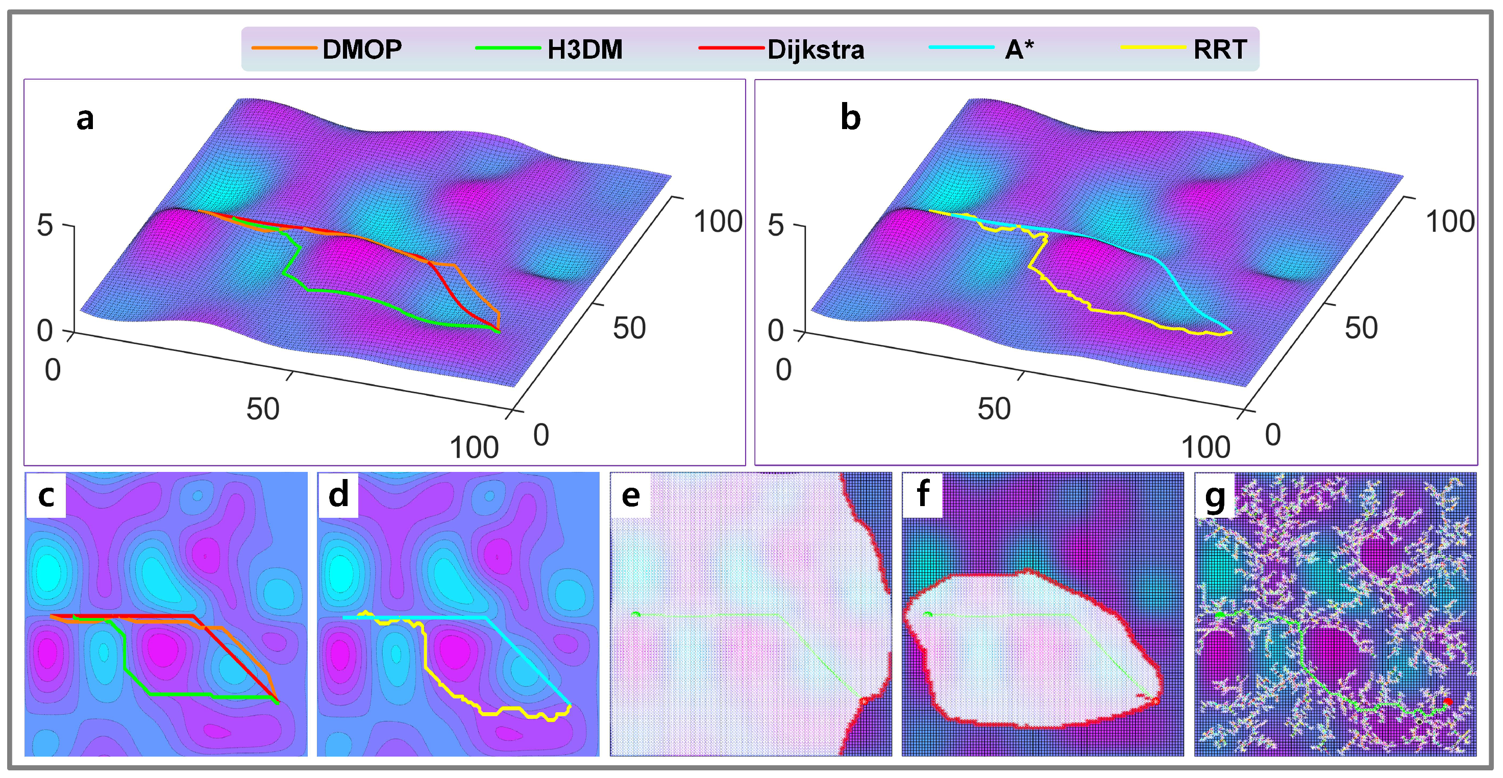
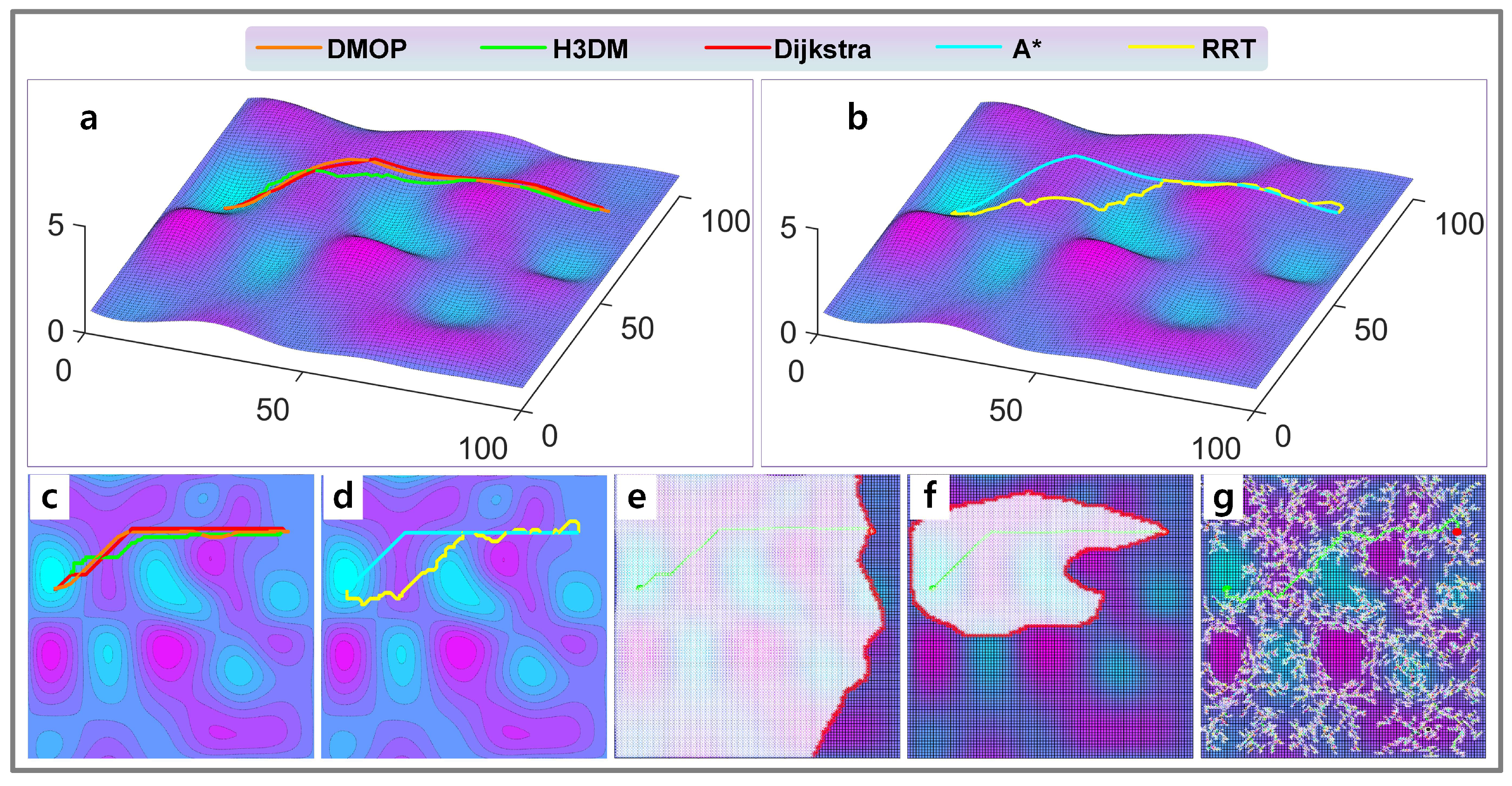
To compare the performance of the DMOP statistically, we conducted 200 path planning experiments with random starting points and destinations and then choose five representative cases to demonstrate the effectiveness of the method. The plots in
Figure 6 illustrate the simulation result for each algorithm. In
Figure 6a, the points represent the performance of various algorithms in terms of time, energy consumption, and path distance in the planning task. For ease of data visualization, we have taken the logarithm of time values, making the scatterplot distribution more concentrated. Furthermore, points closer to the lower-right corner indicate lower energy consumption, shorter path distance, and search time. In this three-dimensional graph, it is easy to observe that, overall, DMOP significantly reduces search time, exhibiting low energy consumption and short path length. In
Figure 6b, the vertical axis represents the sum of path length and energy consumption, where a smaller value indicates higher path quality in the search. Due to its breadth-first search mechanism, Dijkstra’s algorithm can find the global optimum path in this task. However, its search mechanism also results in much longer search time. In contrast, DMOP manages to significantly reduce search time while maintaining path quality similar to that of the Dijkstra’s algorithm. From a large volume of numerical statistics, we can observe that the DMOP method demonstrates excellent stability and performance.
From the results, we can see that the planning speed of DMOP is extremely fast, which is around 0.32 s, and the quality of its results is very close to those of the Dijkstra method. The Dijkstra method can obtain the global optimal paths but needs about 100 s or more; thus, its efficiency is low. The A* method often takes dozens of seconds to complete the planning. The RRT is very slow and unstable (Case 2 takes 3271 s to find the target, while Case 3 takes 958 s), the global nature of the planned results is average, and the path smoothness is poor. The time required for H3DM to complete the planning task is around 10 s, and the global nature of the paths it plans is a bit worse than that of DMOP. Though DMOP does not find the global optimal solution, its path quality is close to that of the A* method. Considering the search speed and the path quality, the efficiency of DMOP is the best among all the methods.
Overall, if we assume that the paths planned by the DMOP, A*, and H3DM are all acceptable, then the DMOP is over 100 times faster than the A* method and about 30 times faster than the H3DM.
5.2. Discussion
The simulation results show that although the Dijkstra method can find the global optimal path, it always searches almost the whole map to obtain the result. The A* method is recognized as the most efficient method for the single-objective path planning task on 2D maps, which takes less time and has a high quality of solution because of the added heuristic function. In the 2.5D multi-objective path planning task, the A* method still maintains high efficiency. However, we made a special design of the heuristic function of the A* method according to the planning task of this paper to achieve relatively stable results. The special design is that we model its heuristic function with linear distance, curvilinear distance, and energy consumption estimation and set appropriate parameters. For the RRT algorithm, there are blindness and randomness in its search, which leads to its inefficiency and the poor smoothness of the planned paths. From the figures of the results, we can see that RRT searches fewer points compared to the Dijkstra method, but its search area basically covers the whole map.
Whether it is the Dijkstra method, A*, or RRT, they all need to search a certain area, causing the method to take a significant amount of time. The H3DM is built on the idea of pure heuristics, and the algorithm tends to be pure greedy search, with the least number of search points for path planning, so its efficiency is much higher than the previous methods, and the method takes only about 10 s. Due to the extreme compression of the search space, it sacrifices the quality of the solutions to some extent. However, in general, the solution obtained from H3DM does not undergo significant sacrifices, and the time required to plan the path is further reduced, thus indicating an improvement.
Compared with these previous methods, a large number of statistical data show that the DMOP method has a relatively high quality of solution and a very short search time. For the global nature of the solution of DMOP, during the training process DQN learns to judge the peaks and valleys, and it always sees the global view (the whole map as input), which allows it to achieve global path planning from another perspective. Furthermore, through many training tasks, DQN learns to assess the cost of each point in the planning process from a global perspective and thus plan paths that are better globally. For the search time, theoretically, the DMOP method searches the same region as the H3DM method does, and both methods perform greedy selection planning from neighbor points each time. However, due to the complexity of the heuristic function model in the H3DM, it takes a significant amount of time to estimate the cost of each neighbor point. On the other hand, the DMOP requires only simple forward operations, and the calculations inside the network are straightforward, which makes the method very fast.
Furthermore, DMOP is tested on the tasks that it has never seen before. Another important conclusion we can draw from the simulation is that this method possesses robust reasoning capabilities and adaptability to various planning tasks, allowing it to perform any untrained planning task on a given map. On this basis, for exploration robots working on a specific terrain area, the DMOP method can learn to plan paths on this area in advance and quickly generate the navigation path for robots while they are working.
6. Conclusions and Prospect
In this paper, a deep reinforcement learning-based multi-objective 2.5D path planning method is investigated for the energy-saving of ground vehicles. Such a method can efficiently plan paths that have a good trade-off for distance and energy consumption. In the implementation, we solved two technical problems: the convergence problem of DQN in high state space, and realizing multi-objective path planning. Unlike traditional algorithms, the DMOP method does not have a search area, and it directly generates the planned path after loading the map, which has high efficiency and path quality. Simulation shows the proposed method is over 100 times faster than the A* and about 30 times faster than the H3DM method. Also, simulation proves the method has powerful reasoning capability that enables it to perform arbitrary untrained planning tasks on the map where the ground vehicles are required to operate.
Future work will involve the following: (1) studying a new deep reinforcement learning method that converges more quickly than the DQN; and (2) exploring the application of deep reinforcement learning in solving other path planning problems.
