Magnetic Flux Leakage Testing Method for Pipelines with Stress Corrosion Defects Based on Improved Kernel Extreme Learning Machine

Abstract

This study aims to study the safety of oil and gas pipelines under stress corrosion conditions and grasp the corrosion damage situation timely and accurately. Consequently, a non-destructive testing method combining magnetic flux leakage testing technology and a kernel function extreme learning machine improved by genetic algorithm (GA-KELM) is proposed. Firstly, the variation of the corrosion defect dimension and profile with time is obtained by numerical simulation. At the same time, the distribution of the magnetic flux leakage signal under different defect conditions is analyzed and studied. Finally, feature selection is carried out on the magnetic flux leakage signal distribution curve, and GA-KELM is used to predict the depth and length of corrosion defects so as to realize the non-destructive testing of the pipeline defects. The results show that different geometric features result in different magnetic flux leakage signal distributions. There is a corresponding relationship between the defect dimension and extreme value, area, and peak width of the magnetic flux leakage signal distribution curve. The GA-KELM prediction model can effectively predict the depth and length of corrosion defects, and the prediction accuracy is better than the traditional extreme learning machine prediction model.

1. Introduction

It is well known that pipeline transportation is a secure, dependable, and economical means of energy conveyance, which is increasingly used in the transportation of oil and gas resources around the world. The corrosion of metal pipelines is due to the difference in electrode potential, and electrochemical reactions occur when the metal is in contact with the electrolyte. Pipelines are affected by a variety of stresses during service, such as soil stress, internal residual stress of the pipelines, thermal stress caused by welding, etc. [1]. Both elastic and plastic tensile stress can improve the surface activity of pipeline steel, further promote the electrochemical reaction of the steel surface, and accelerate the corrosion of pipelines [2]. Corrosion is a dynamic process that develops over time, and as the operating time of pipelines increases, corrosion will become a major hidden danger to the safe operation of pipelines. There are several methods to predict the damage to pipelines such as experiments, analytical methods and the finite element method (FEM). Recently, with the advancement of computer technology, FEM has established itself as the method of choice for the majority of analysis applications [3]. Khalajestani K.M [4] used FEM to analyze the residual strength of pressure pipelines with corrosion defects, and the research results proved that the depth and length of defects and the spacing between adjacent defects had a greater impact on the residual strength of pipelines. Larin [5] used FEM to analyze and determine the local area of the maximum stress, and found that the stress state was affected by the internal pressure and time of the corroded defective pipelines. Mourad Nahal [6] established a numerical model of a corroded elbow by FEM, studied the mechanical behavior under the action of corrosion defects, and established an empirical model. The results show that the failure probability is proportional to the corrosion rate, the reliability of a corroding pipe elbow can be significantly affected by corrosion and residual stress. Zhang Jia [7] used FEM to carry out nonlinear analysis of buried natural gas pipelines. The effects of internal pressure, corrosion pit defect size, internal and external wall corrosion, the corrosion pit group, and different types of volumetric corrosion pit defects on the failure of an L360QS steel pipe were analyzed with consideration to the effects of axial and circumferential zones of corrosion pits.

To guarantee the secure functioning of pipelines, periodic inspections are imperative to assess their corrosion status. Magnetic flux leakage testing is a significant non-destructive testing method that is widely used. When combined with other methods, it provides a fast and inexpensive evaluation of ferromagnetic workpieces. Given that a substantial proportion of oil and gas conveyance pipelines are fabricated from ferromagnetic materials, magnetic flux leakage testing technology can detect the location and dimension of pipeline defects effectively [8]. Magnetic flux leakage testing technology evolved from magnetic particle detection technology as early as 1906 in C. Mc Cann’s work in South Africa, and other scholars have carried out flaw detection by magnetization for the problem of broken wire ropes. In 1933, Zuschlug first proposed the method of detecting leakage magnetic fields using magnetic sensitive elements. In 1947, Hastings designed the first magnetic flux leakage testing system, and then magnetic flux leakage testing and its defect magnetic flux leakage imaging technology began to be applied [9]. In recent years, magnetic flux leakage testing technology has gradually become a popular research direction for scholars [10,11,12,13,14,15,16]. Z. Usarek [17] designed a FLUMAG500 magnetic flux leakage testing device for the detection of corrosion defects on gas pipe walls. An advanced signal processing and analysis system was developed for the device, and the working principle of the device was introduced. Miguel A. Machado [18] developed a new eddy current probe for detecting micron-level defects in any direction on the inner surface of the pipelines and verified the performance of the designed probe. Yavuz Ege [19] developed a new magnetic flux leakage testing system for natural gas and long-distance oil transportation pipelines with a KMZ51 AMR sensor. Tohara Makoto [20] proposed a method to obtain the outer surface defects of ferromagnetic steel pipelines by detecting the changes in the eddy current distribution in the pipelines. Zhao Yunli [21] used ANSYS Maxwell software to calculate the permeability of different specifications at the inner and outer walls of X80 steel pipelines and verified the calculation results. Hu Jing [22] studied the distribution law and modeling method of a vortex magnetic flux leakage field on the inner and outer walls of pipelines, constructed a mathematical model of a dynamic magnetic flux leakage similar stability field for defects on the inner and outer walls of pipelines, explored the identifiability of magnetic flux leakage signal features under dynamic conditions, selected the data characteristics of defect signals on the inner and outer walls, and established an effective method for distinguishing between internal and external defect signals. Zheng Fuyin [23] mathematically modeled the force–magnetic coupling relationship of ferromagnetic materials, derived the functional relationship between stress and material permeability, designed a pipeline stress detection system, and gave the mathematical relationship between the magnetic flux leakage signal on the pipe surface and the magnetic permeability of the material, excitation voltage and coil turns. Feng Bo [24] presented a comprehensive review of magnetic flux leakage (MFL) testing, explained the principle of MFL testing with the refraction magnetic field theory, and analyzed the factors affecting the MFL test signal. The results show that excitation and sensing are the most important steps in MFL testing, in which excitation decides if there is a leakage field generated and sensing decides if the generated field can be effectively detected.

Artificial neural networks have undergone rapid development in recent years, and achieved great success in tasks such as classification and regression. The emphasis of non-destructive testing is the quantification and prediction of defects, which is essentially a classification or regression problem. Thus, artificial neural networks have been widely used in defect quantification and prediction. Chen Yuanhang presented a method based on feature extraction and machine learning algorithms for online quality monitoring and defect classification, and experiments indicated the performance of artificial neural networks is slightly better than that of support vector machines, while both of them have their own advantages [25]. Feng Jianghua proposed a novel object detection algorithm to detect rail defects. The net architecture of the proposed algorithm includes a backbone network using MobileNet and several novel detection layers [26]. Mat Jizat Jessnor Arif described an evaluation of machine learning classifiers to be applied in wafer defect detection—k-nearest neighbours, logistic regression, stochastic gradient descent, and support vector machine were evaluated with three defect categories and one non-defect category [27]. Sun Hongyu integrated the magnetic flux leakage theory into the loss function and proposed a physics-informed double-fed cross-residual network that estimated the defect length, width, and depth accurately [28]. Wang Qi proposed an extreme learning machine optimized by a genetic algorithm to predict the erosion rate, residual life, and residual strength of the pipe with erosion defects; the model can not only predict effectively, but its prediction accuracy is better than the traditional model [29].

As mentioned above, the presence of corrosion defects constitutes one of the main threats to pipeline safety. The soil-induced strain, combined with internal pressure, results in a complex stress/strain condition on pipelines. The local stress concentration developed at the defect further accelerates the localized corrosion. Magnetic flux leakage testing technology can effectively detect the corrosion damage of pipelines. Meanwhile, artificial neural networks are widely used in the quantification and prediction of defects. However, most of the existing research uses the experimental method to carry out the research of magnetic flux leakage testing, and there is no close connection with computer technology. In order to assess the corrosion damage of oil and gas pipelines from the perspective of safety and economy, it is imperative to establish a scientific evaluation methodology. In this paper, considering the combined impacts of corrosion and stress on oil and gas pipelines in practical engineering scenarios, the finite element model of pipeline stress corrosion is established. Employing time as a variable, the dynamic evolution of corrosion defect profiles and sizes with pipelines is investigated. Building upon the principles of magnetic field theory, the finite element model of magnetic flux leakage testing for pipeline defects is established. It enables an exploration of the magnetic flux leakage signal distribution under varying corrosion defect profiles; the effects of defect depth, defect length and lifting height on magnetic flux leakage signal distribution are also analyzed. On this basis, the features of the signal distribution curve are defined and selected as sample data, and the GA-KELM model is built to predict the depth and length of defects. The above contributes to advancing the theoretical foundations of corrosion protection strategies for oil and gas pipelines in engineering applications.

2. Numerical Simulation Analysis of Pipelines Stress Corrosion

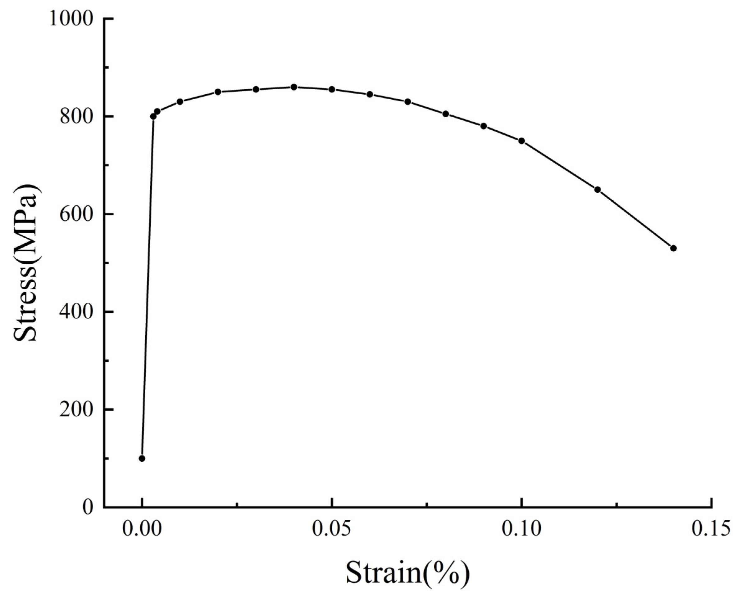
2.1. Simulation of Elastoplasticity

Elastoplasticity refers to the deformation of an object when it is subjected to external force; only part of the deformation disappears when the external force is removed, and the rest will not disappear by itself. Elastoplasticity includes elastic mechanics and plastic mechanics; in the scope of elastic mechanics, stress and strain are linearly related, while in the scope of plastic mechanics, the relationship between stress and strain is nonlinear. This nonlinear characteristic is related to the materials studied, and has different transformation laws for different materials and conditions. The model established in this paper adopts the small strain plastic model to simulate the elastic–plastic mechanics of the pipelines and the isotropic hardening model, whose hardening function ${\sigma }_{yhard}$ (a function that describes the stress–strain curves in the scope of plasticity) is defined as follows:

$${\sigma }_{yhard}={\sigma }_{\exp }\left({\epsilon }_p+\frac{{\sigma }_e}{E}\right)-{\sigma }_{ys}$$

(1)

In Equation (1), ${\sigma }_{\exp }$ is the stress–strain curve measured by X100 pipeline steel experiments [30], as shown in Figure 1; ${\epsilon }_p$ is plastic deformation; ${\sigma }_e$ is the von Mise stress; $E$ is the Young’s modulus, 2.07 × 10⁹ Pa; ${\sigma }_{ys}$ is the yield strength of the pipeline steel, 8.06 × 10⁸ Pa.

2.2. Simulation of Electrochemical Corrosion

Corrosion of oil and gas pipelines refers to the destruction of the outer wall of oil and gas pipelines due to chemical changes, electrochemical changes or physical dissolution of metal pipelines under long-term contact with surrounding substances. Soil is the main cause of the corrosion of buried pipelines. Because the soil contains a lot of water and air, water makes the soil become a conductor, and the airflow causes the uneven distribution of oxygen concentration, and finally forms the galvanic cell. The pipelines are dissolved as the anode, which is damaged [31].

The model dictates that two electrochemical reactions, iron dissolution (anode) and hydrogen evolution (cathode), occur on the corrosion defect surface of the pipelines, and the other surface of the pipelines is considered to be electrochemically inert. The chemical reaction formula of the anode reaction and the cathode reaction is as follows:

$$\mathrm{Fe}\to {\mathrm{Fe}}^{2+}+2\mathrm{e}$$

(2)

$${\mathrm{H}}^{+}+\mathrm{e}\to \mathrm{H}$$

(3)

The anode’s Tafel expression is used to simulate the iron dissolution reaction, and the local anode current density $i_a$ is defined as follows [32]:

$$i_a=i_{0,a}{10}^{\frac{{\eta }_a}{A_a}}$$

(4)

$${\eta }_a={\phi }_s-{\phi }_l-E_{eq,a}$$

(5)

$$E_{eq,a}=E_{eq0,a}-\frac{\Delta P_m{V}_m}{zF}-\frac{TR}{zF}\ln \left(\frac{v\alpha }{N_0}{\epsilon }_p+1\right)$$

(6)

In Equations (4)–(6), $i_{0,a}$ is the exchange current density, 2.353 × 10⁻³ A/m²; $A_a$ is the anode’s Tafel slope, 0.118 V; ${\eta }_a$ is the overpotential of the anode reaction; $E_{eq,a}$ is the equilibrium potential of the anode reaction; $E_{eq0,a}$ is the standard equilibrium potential of anode reaction, −0.859 V; $\Delta P_m$ is the overpressure that causes elastic deformation, 2.687 × 10⁸ Pa; $V_m$ is the molar volume of steel, 7.13 × 10⁻⁶ m³/mol; $z$ is the electric charge of steel, 2; $F$ is Faraday’s constant; $T$ is the absolute concentration, 298.15 K; $R$ is the ideal gas constant; $v$ is the directional correlation factor, 0.45; $\alpha$ is the coefficient, 1.67 × 10¹⁵ m⁻²; $N_0$ is the initial dislocation density, 1 × 10¹² m⁻².

The cathode’s Tafel expression is used to simulate the hydrogen evolution reaction, and the local cathode current density $i_c$ is defined as follows [32]:

$$i_c=i_{0,c}{10}^{\frac{{\eta }_c}{A_c}}$$

(7)

$$i_{0,c}=i_{0,c,ref}{10}^{\frac{{\sigma }_e{V}_m}{6F(-A_c)}}$$

(8)

$${\eta }_c={\phi }_s-{\phi }_l-E_{eq0,c}$$

(9)

In Equations (7)–(9), $i_{0,c}$ is the exchange current density; $A_c$ is the cathode’s Tafel slope, 0.207 V; $i_{0,c,ref}$ is the reference exchange current density of the cathode reaction without external stress/strain, 1.457 × 10⁻² A/m²; ${\eta }_c$ is the overpotential of the cathode reaction; $E_{eq,c}$ is the standard equilibrium potential of the cathode reaction, −0.644 V.

Deformation geometry is used to model the dissolution of iron in corrosion defects. The dissolution of iron causes the electrode boundary to move at a speed of $v$, calculated by the following equation [33]:

$$v=\frac{i_a}{2F}\frac{M}{\rho }$$

(10)

In Equation (10), $M$ is the molar mass of iron, 55.845 g/mol; $\rho$ is the density of iron, 7870 kg/m³.

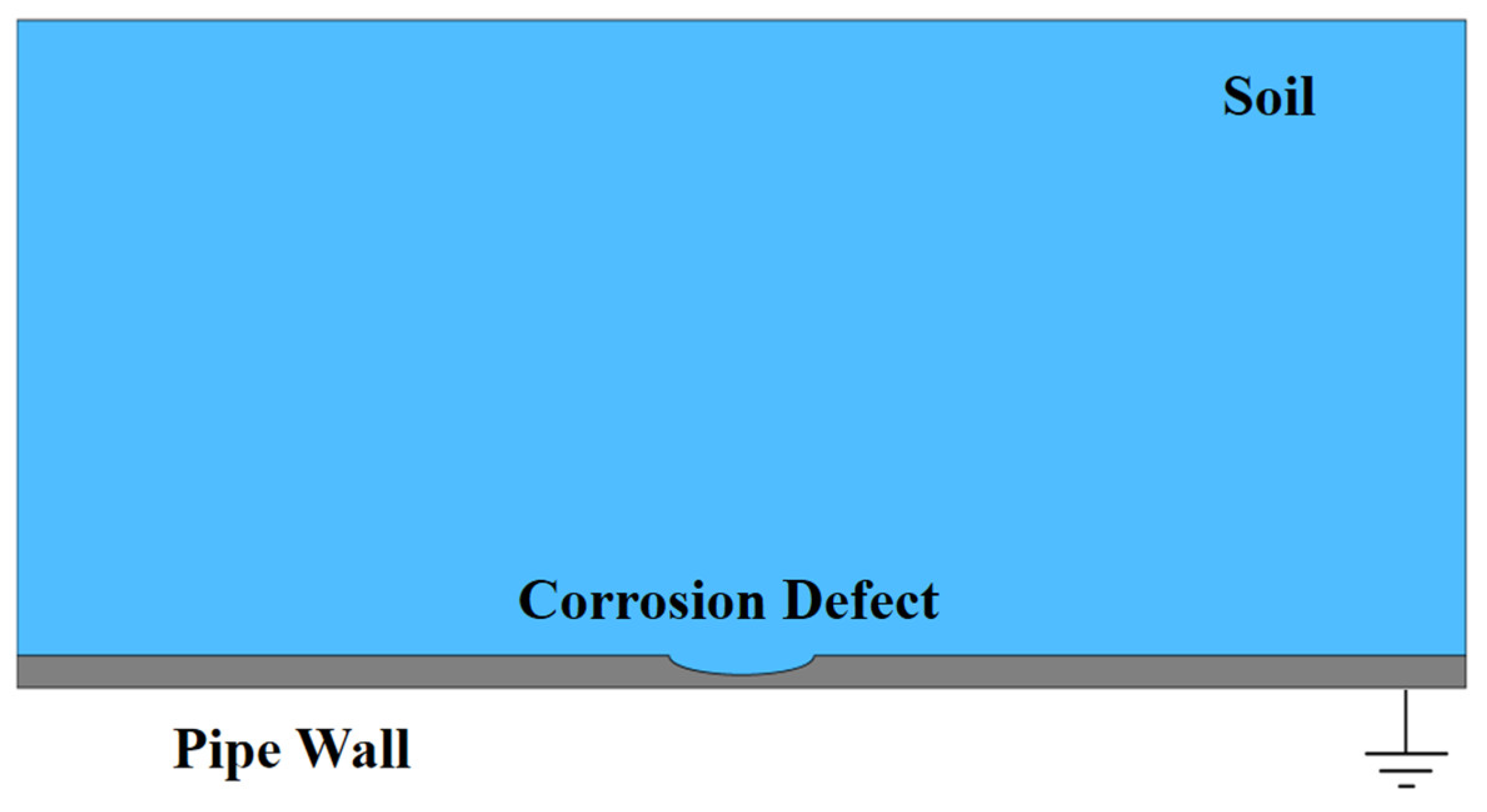
2.3. Finite Element Model of Pipelines Stress Corrosion

COMSOL Multiphysics 6.0 is used to establish a finite element model of pipeline stress corrosion. The geometric model consisted of X100 pipelines and the surrounding soil domain, as shown in Figure 2. The pipe wall thickness is 19.1 mm, and the length of the pipe segment used for finite element simulation is 2 m. The initial corrosion defect is elliptical, with a length of 200 mm and a depth of 60% of the pipe wall thickness, 11.46 mm. In numerical simulation, the calculation speed and accuracy are affected by the quality and quantity of the mesh; high-quality mesh can not only reduce the operation memory, but also improve the calculation accuracy. This paper uses a free triangle mesh to divide the corrosion defect area’s local mesh encryption and set the maximum unit size of 1 mm. The complete mesh consists of 13,807 cells, with a maximum cell size of 40 mm, a minimum cell size of 0.6 mm, and a maximum cell growth rate of 1.2. The contact interface between the pipeline and the soil domain is set as a free boundary, an electrochemical corrosion reaction occurs, and the conductivity of the electrolyte in the soil domain is 0.096 S/m. The left end of the pipeline is fixed, the right end is subjected to tensile strain, and the bottom of the pipeline is set to electrical ground.

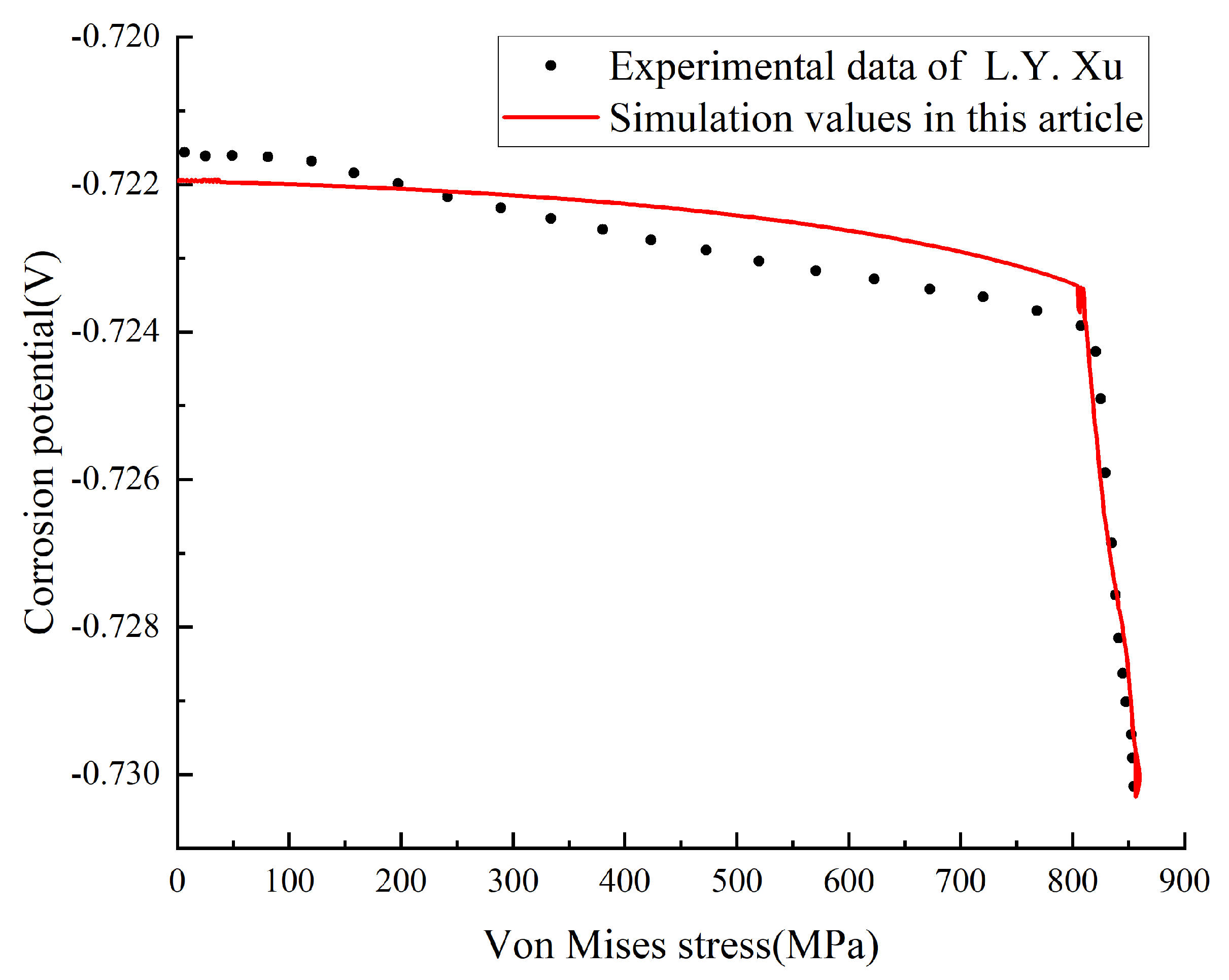
2.4. Verification of Model Accuracy

Corrosion potential is the potential measured when a metal reaches a steady state of corrosion in the absence of an applied current. It is the mixed potential of anodic and cathodic reactions polarized by self-corrosive currents, which greatly affects the corrosion of metals [34]. Before the numerical simulation, the rationality and accuracy of the finite element model should be verified. The curve of the corrosion potential change with von Mises stress of X100 pipeline steel is shown in Figure 3, and a comparison between the experimental data in the literature and numerical simulation results is shown in

Table 1. Comparison of experimental data and simulation results.

Von Mises Stress (MPa)	Corrosion Potential in Literature (V)	Corrosion Potential of Simulation (V)	Error (%)
6.116	−0.72154	−0.72195	0.057
25.446	−0.72156	−0.72193	0.051
51.218	−0.72163	−0.72197	0.048
82.364	−0.72163	−0.72199	0.050
121.024	−0.72167	−0.72201	0.046
159.681	−0.72178	−0.72203	0.035
199.409	−0.72195	−0.72206	0.015
243.432	−0.72213	−0.72209	0.004
289.603	−0.72230	−0.72213	0.023
334.701	−0.72245	−0.72218	0.037
381.947	−0.72260	−0.72224	0.050
427.047	−0.72273	−0.72230	0.059
474.295	−0.72286	−0.72237	0.067
522.613	−0.72305	0.72245	0.083
570.937	−0.72314	−0.72255	0.081
622.480	−0.72327	−0.72268	0.082
672.950	−0.72340	0.72283	0.079
721.271	−0.72353	−0.72298	0.076
768.518	−0.72368	−0.72318	0.069
808.242	−0.72389	−0.72361	0.039
820.036	−0.72424	−0.72526	0.141
827.514	−0.72490	−0.72640	0.207
831.748	−0.72593	−0.72681	0.121
835.988	−0.72687	−0.72724	0.051
838.093	−0.72758	−0.72745	0.017
843.433	−0.72809	−0.72790	0.026
846.623	−0.72863	−0.72824	0.053
849.819	−0.72905	−0.72862	0.059
851.948	−0.72938	−0.72899	0.052
854.070	−0.72980	−0.72943	0.051
856.197	−0.73015	−0.73029	0.020

. It can be seen from the data analysis that the numerical simulation results in this paper fit well with the experimental data of L.Y. Xu [35], with a maximum error of 0.27%, a minimum error of 0.04%, and an average error of 0.059%. The results show that the finite element model can simulate the pipeline stress corrosion accurately, and the mesh division and boundary condition setting are reasonable and feasible.

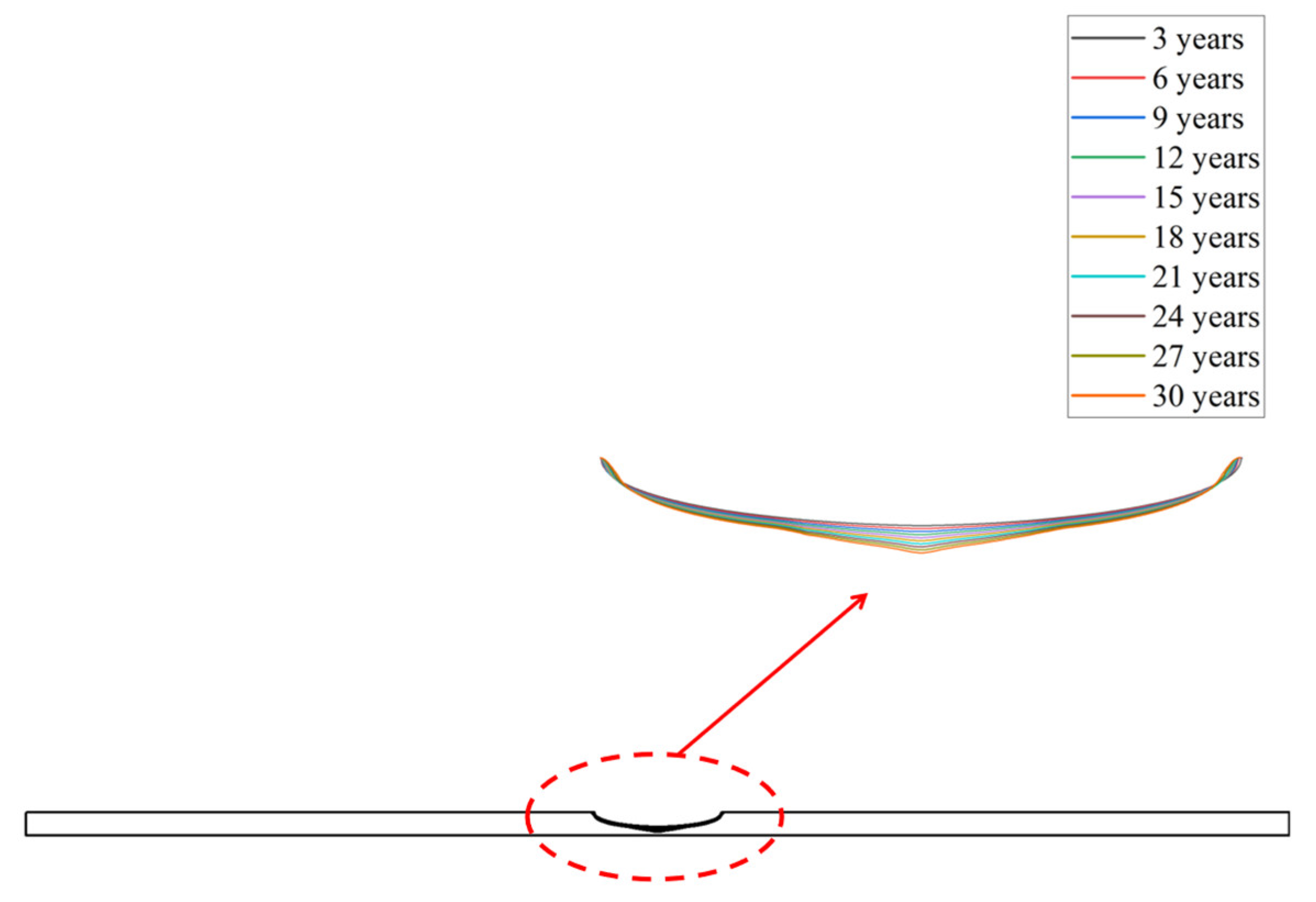
2.5. Simulation Analysis of Corrosion Situations

This paper undertakes a comprehensive analysis of pipeline corrosion over a 30-year period, with calculations performed at 3-year intervals. A total of 10 simulations have been conducted to assess the progression of corrosion in the presence of defects. The evolution of defect dimensions over the corrosion timeline is presented in

Table 2. Change of defect dimension with corrosion time.

Corrosion Time (Years)	Defect Depth (mm)	Defect Length (mm)
3	11.981	200.569
6	12.507	201.243
9	13.041	202.017
12	13.580	202.888
15	14.122	203.857
18	14.662	204.925
21	15.199	206.104
24	15.733	207.419
27	16.266	208.909
30	16.798	210.649

, and the transformation of defect profiles is depicted in Figure 4. Analysis of the data shows that the corrosion defect changed significantly. The depth of defects increased from 11.46 mm to 16.798 mm, with an average increase of 0.54 mm every three years. The length of defects increased from 200 mm to 210.649 mm, with an average increase of 1.065 mm every three years. With the increase in the service life of pipelines, the stress corrosion leads to the continuous thinning of the pipe wall and the increase in the defect area, which seriously threatens the safe operation of pipelines.

The initial corrosion defect depth of 11.46 mm is kept unchanged, and the initial defect lengths are taken as 160 mm, 170 mm, 180 mm, 190 mm, 200 mm, 210 mm, 220 mm, 230 mm, 240 mm and 250 mm, respectively. By establishing a model and calculating the defect profiles under different corrosion times, they are derived to provide a geometric model for the subsequent numerical simulation analysis of magnetic flux leakage testing signal detection.

3. Numerical Simulation Analysis of Magnetic Flux Leakage Testing

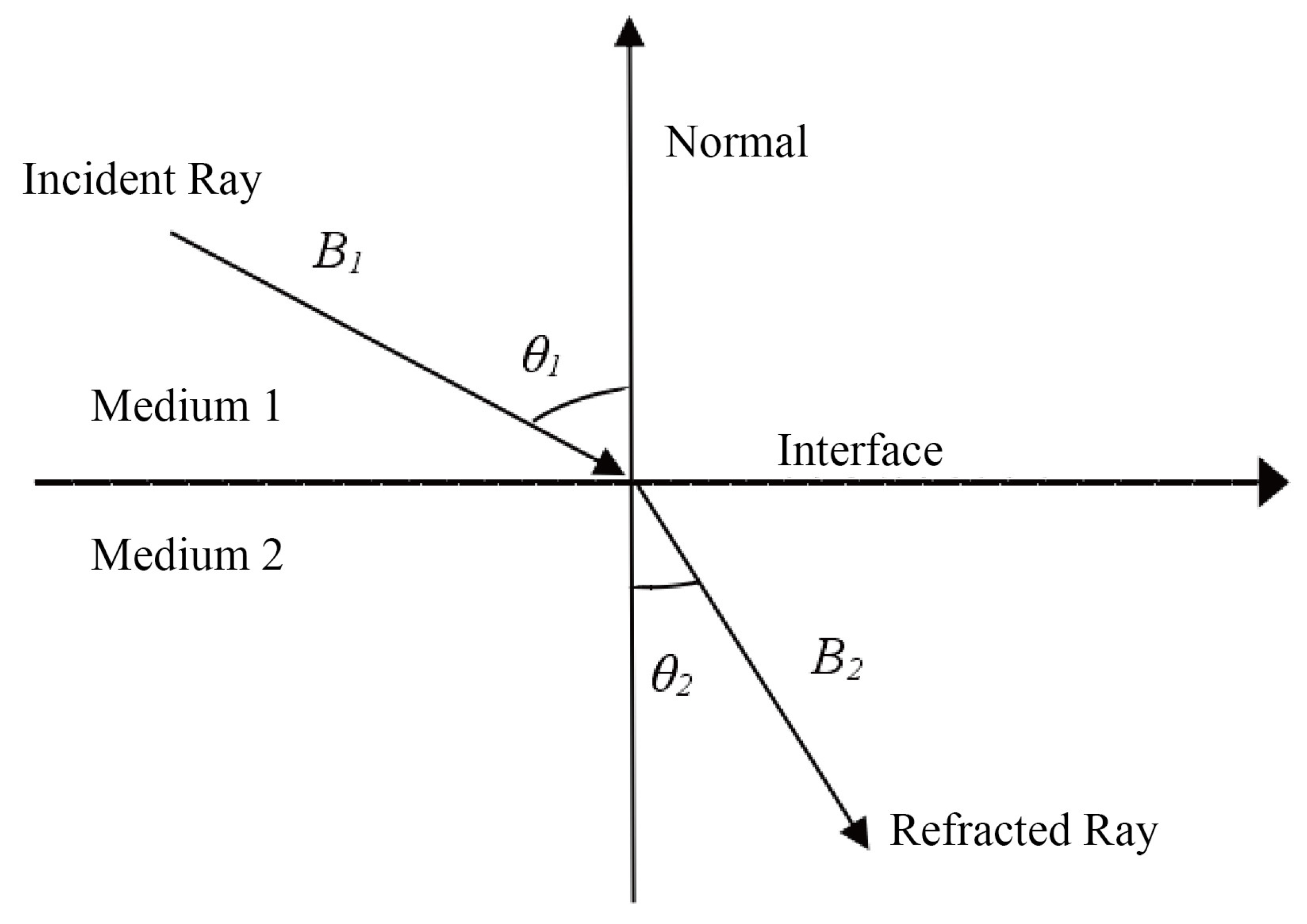
3.1. Magnetic Flux Leakage Testing Theory

Similar to electric field lines, magnetic induction lines are imaginary curves used to help describe the direction of a magnetic field. The propagation of magnetic induction lines obeys the boundary conditions of the electromagnetic field. When the magnetic induction line passes through the different media interfaces of the two materials, the propagation path is refracted due to the change in permeability [36]. A schematic diagram of the refractive law of the magnetic induction line is shown in Figure 5.

As shown in the figure, two media with different permeability are divided by interface, and the normal components of magnetic induction intensity in medium 1 and medium 2 are $B_{1n}$ and $B_{2n}$, respectively. The magnetic field strength components of the circumferential of medium 1 and medium 2 are $H_{1t}$ and $H_{2t}$, respectively, the angle between magnetic induction and normal is ${\theta }_1$ and ${\theta }_2$, and the permeability of medium 1 and medium 2 is ${\mu }_1$ and ${\mu }_2$, according to the boundary conditions of the two magnetic media.

$$B_{1n}=B_{2n}$$

(11)

$$H_{1t}=H_{2t}$$

(12)

The permeability ratio on both sides of the medium is equal to the tangent ratio of the angle between the magnetic induction line and the normal line on both sides of the medium, that is:

$$\frac{\tan {\theta }_1}{\tan {\theta }_2}=\frac{{\mu }_1}{{\mu }_2}$$

(13)

The magnetic induction line is incident from medium 1, refracted at the interface and emitted from medium 2; when the size of ${\mu }_1$ is much greater than ${\mu }_2$, ${\theta }_2$ infinitely tends to 0, and ${\theta }_1$ tends to 90 degrees. At this time, the magnetic induction line inside medium 1 becomes very dense and parallel to the interface. The greater the permeability of the material constituting medium 1, the closer ${\theta }_1$ is to 90 degrees.

The principle of magnetic flux leakage testing is schematically shown in Figure 6, where an excitation device is applied to magnetize the pipe wall into near saturation. If the pipe wall is continuous and free of defects, the magnetic induction line will be constrained. The magnetic flux is parallel to the surface of the pipe wall and hardly forms a magnetic field. If there are defects in the pipe wall, the magnetic induction line will change. Part of the magnetic flux leaks into the space on the surface of the pipe wall, forming a leakage magnetic field at the defect. At this time, sensors such as Hall elements are used to detect the magnetic flux leakage on the surface of the pipe wall, and the magnetic flux leakage signal can be analyzed to evaluate whether the pipelines have defects.

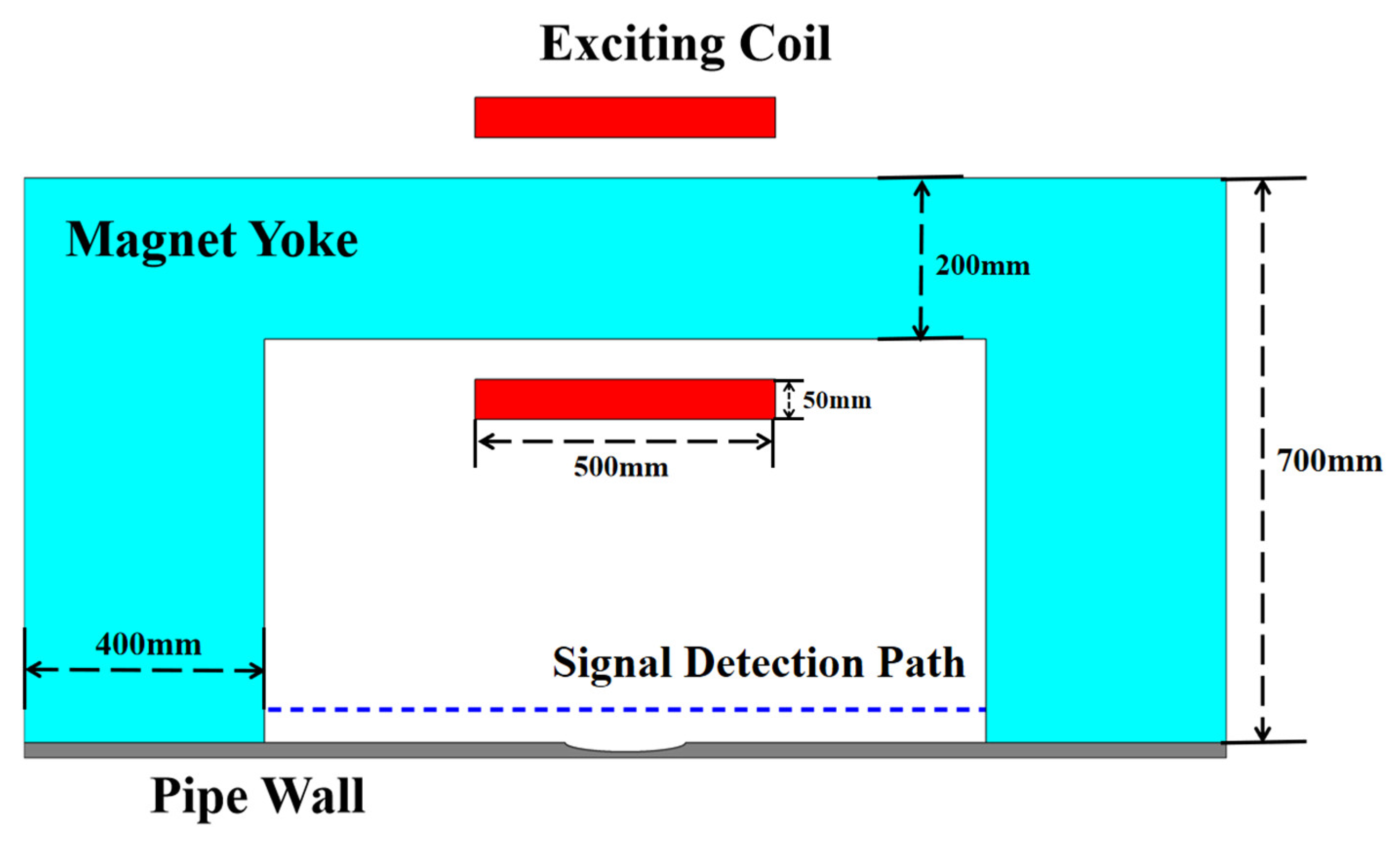
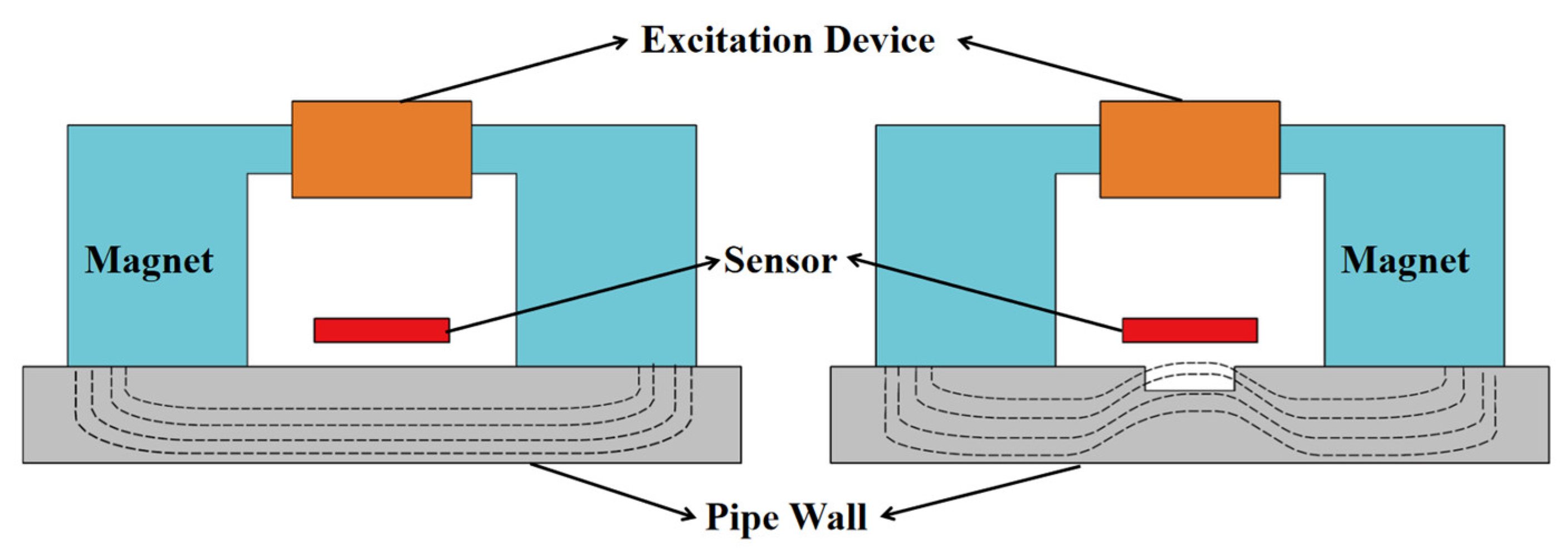
3.2. Finite Element Model of Magnetic Flux Leakage Testing

The finite element model of pipeline defect magnetic flux leakage testing is established by COMSOL Multiphysics 6.0. The geometric model consists of a ferromagnetic X100 steel pipeline, an excitation coil and a magnet yoke. The model adopts the corrosion defect profile calculated in numerical simulation of pipeline stress corrosion, the positions and sizes of the excitation coil and magnet yoke are shown in Figure 7. The magnetic flux leakage signal detection path is set above the pipe wall to replace the Hall sensor, as shown in the blue dashed line. In order to ensure the accuracy and smoothness of the magnetic flux leakage signal, the defect area and the air region above it are divided by a sweeping mesh, the unit size is set to 5 mm, and the rest are divided by a free triangle mesh. The complete mesh consists of 33,990 mesh cells, with a maximum cell size of 60 mm, a minimum cell size of 0.225 mm, and a maximum cell growth rate of 1.2.

In the actual test, considering the geometric size and magnetization effect of the magnetization device, the local magnetization method is generally selected. The magnetic field signal in the magnetization area is detected to determine whether there is a defect in the area and the geometry of the defect. In this paper, the yoke method is selected to locally magnetize the defective pipelines, and the coil is excited to generate the direct current magnetization, which can generate a stable magnetic field without a skin effect. The excitation coil material is set to copper, and the relative permeability is 0.9999912; the yoke material is selected from the COMSOL material library, regardless of loss. The pipeline material is set to X100 pipeline steel with ferromagnetism, and the relative permeability input B-H curve [37] is given as the nonlinearity of the material, as shown in Figure 8.

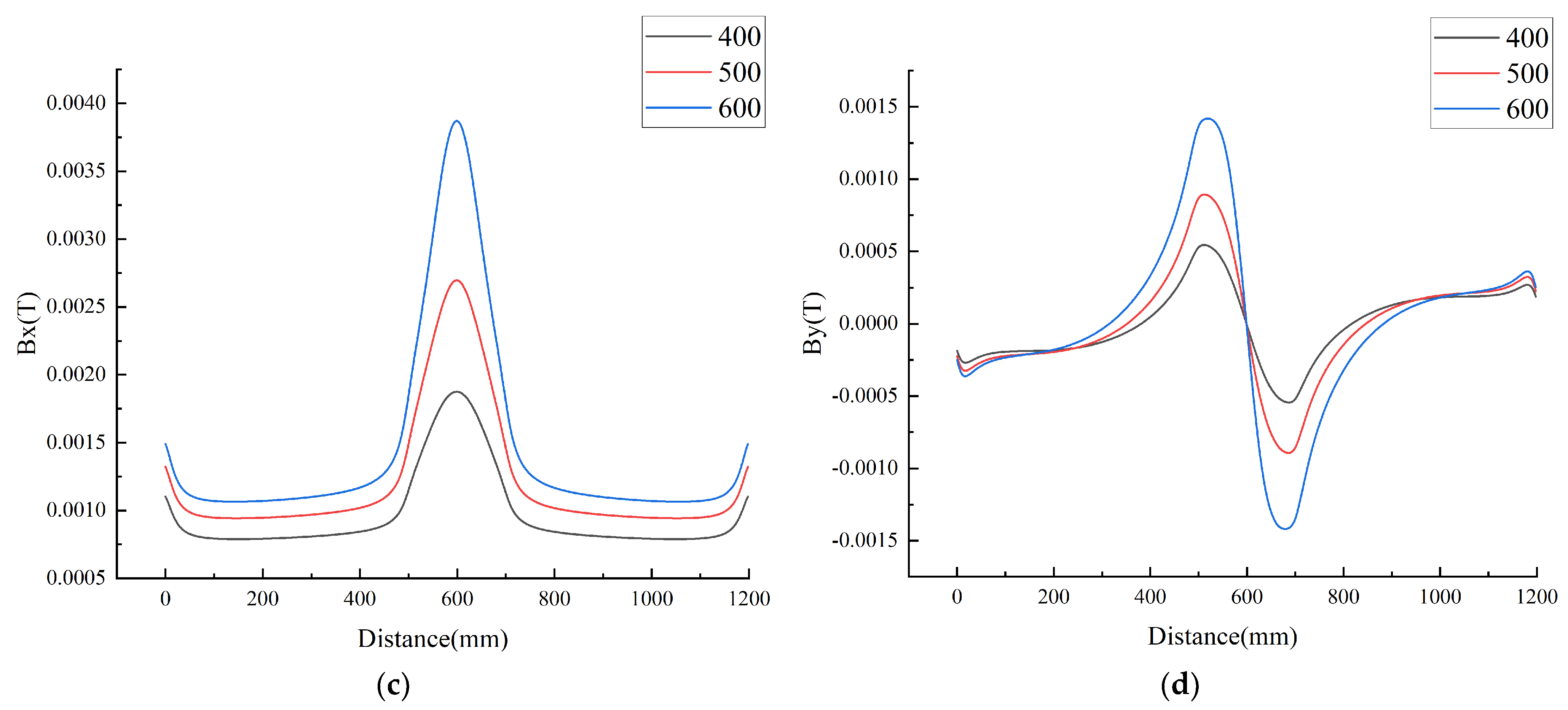
3.3. Effect of Magnet Yoke on Magnetic Flux Leakage Signal

The number of excitation coils and the current value will directly affect the magnetization effect of the magnet yoke. The geometric model with defect length of 200 mm and defect depth of 11.46 mm is established, and the magnetic flux leakage signal detection path is set to 40 mm above the pipe wall. Currents of 3 A, 5 A, and 7 A are applied to the excitation coil, and the coils are wound 400 turns, 500 turns, and 600 turns, respectively. The magnetic flux leakage signal distribution under different parameter conditions is shown in Figure 9:

The figure shows that the magnetization effect of the magnet yoke on the pipe wall will be enhanced with the increase in current value and number of excitation coils. Low current and small coil turns will cause the curve to change less significantly. In the meantime, high current and large coil turns will increase the calculation amount. Therefore, considering the calculation accuracy and calculation speed, a 5A current and 500 coil turns are selected in this study.

3.4. Effect of Geometric Features on Magnetic Flux Leakage Signal

According to the number of excitation coil and current value, the magnetic flux leakage testing model is established, and the influences of defect depth, defect length and lifting height on magnetic flux leakage signal distribution are studied, respectively. When the defect depth is taken as a variable, the magnetic flux leakage signal detection path is set to 40 mm above the pipe wall, the defect length is 200 mm, and the defect depths are taken as 8 mm, 9 mm, 10 mm, 11 mm and 12 mm. When the defect length is taken as a variable, the magnetic flux leakage signal detection path is set to 40 mm above the pipe wall, the defect depth is 11.46 mm, and the defect depths are are taken as 100 mm, 150 mm, 200 mm, 250 mm and 300 mm. When the lifting height is taken as a variable, the defect depth is controlled at 11.46 mm, the defect length remains unchanged at 200 mm, and the magnetic flux leakage signal detection paths are set to 30 mm, 40 mm and 50 mm above the pipe wall. The magnetic flux leakage signal distribution under different geometric characteristics is shown in Figure 10:

The figure shows that different geometric features lead to different magnetic flux leakage signal distributions. As the defect depth increases, the extreme values of the axial and radial components show a continuous increase, with a concomitant increase in the enclosed area of the curve. Conversely, as the defect length increases, the extreme values of both the axial and radial components decrease, accompanied by an increase in the width of the peak of the curve. This observation implies a correlation between the defect dimension and the extreme value, area and peak width of the curve. In addition, the extreme values of the axial and radial components decrease as the lifting height increases. In this study, a lifting height of 40 mm is chosen to ensure clear changes in the distribution curve of the detected magnetic flux leakage signal for each component.

4. Corrosion Defect Regression Prediction

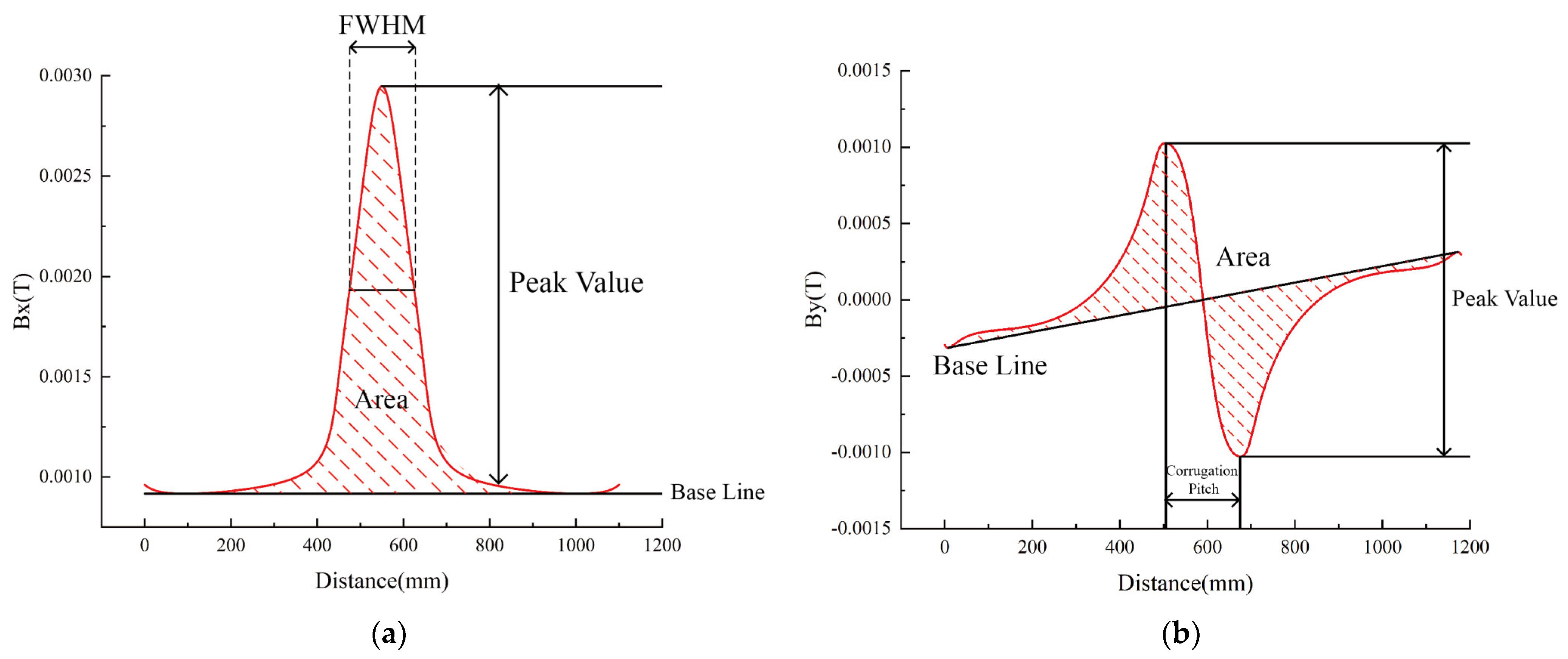
4.1. Magnetic Flux Leakage Signal Feature Extraction

The key to quantitative analysis of defect magnetic flux leakage signal is to extract the feature of the distribution curve. Combined with the above analysis of the transformation law of the magnetic flux leakage signal curve, the feature of the distribution curve is defined as follows (Figure 11):

1.

Peak value

A baseline is established along the lower edge of the axial component curve, and the disparity between the peak of the curve and this baseline is defined as the peak value of the axial component (P₁). In the meantime, the disparity between the positive peak and the negative peak within the radial component curve is defined as the peak value of the radial component (P₂).

2.

Area

A baseline is established along the base of the axial component curve, and the absolute area enclosed by the curve and the baseline is defined as the peak area of the axial component (A₁). Similarly, by connecting the endpoints of the radial component curve to form a baseline, the absolute area enclosed by the curve and the baseline is defined as the peak area of the radial component (A₂).

3.

Full width at half maximum (FWHM)

The width of the axial component curve at half of its peak height is defined as the FWHM of the axial component (W₁). On the other hand, since the radial component curve exhibits two peaks, the average of two width values is defined as the FWHM of the radial component (W₂).

4.

Corrugation pitch

By calculating the disparity between the abscissa values of the negative and positive peaks of the radial component curve, the resulting difference is defined as the corrugation pitch of the radial component (S).

The magnetic flux leakage signal distribution of pipelines with different defect profiles is calculated by using the magnetic flux leakage testing model. A total of 100 groups of data are obtained by extracting the feature of the distribution curve, as shown in

Table A1. The feature of magnetic flux leakage signal distribution curve.

Defect Depth	Defect Length	P1	A1	W1	P2	A2	W2	S
12.073	160.530	0.0021	0.3001	126.946	0.0021	0.3156	116.439	1164.044
12.671	161.141	0.0024	0.3314	121.415	0.0024	0.3660	119.899	1164.067
13.263	161.852	0.0028	0.3694	114.366	0.0027	0.4283	123.430	1164.091
13.852	162.612	0.0032	0.4150	106.596	0.0031	0.5037	126.542	1164.051
14.440	163.463	0.0037	0.4625	100.618	0.0035	0.5818	128.045	1166.076
15.027	164.388	0.0043	0.5163	95.281	0.0041	0.6708	128.343	1166.042
15.618	165.411	0.0049	0.5746	91.095	0.0047	0.7672	128.040	1166.075
16.214	166.518	0.0056	0.6364	88.083	0.0053	0.8687	127.563	1168.043
16.811	167.752	0.0062	0.7026	85.895	0.0060	0.9771	127.142	1168.079
17.412	169.133	0.0069	0.7740	84.344	0.0067	1.0933	126.868	1170.059
12.052	170.536	0.0021	0.3080	132.375	0.0021	0.3142	116.383	1164.044
12.637	171.160	0.0023	0.3381	126.743	0.0023	0.3648	119.851	1164.067
13.216	171.874	0.0027	0.3749	119.241	0.0026	0.4275	123.411	1165.002
13.791	172.672	0.0031	0.4173	111.344	0.0030	0.5033	126.526	1164.048
14.361	173.553	0.0036	0.4654	104.007	0.0034	0.5811	128.020	1165.077
14.930	174.519	0.0041	0.5144	98.674	0.0039	0.6712	128.353	1165.043
15.498	175.575	0.0047	0.5697	93.907	0.0045	0.7681	128.064	1166.080
16.067	176.739	0.0053	0.6284	90.372	0.0051	0.8705	127.611	1166.967
16.642	178.035	0.0060	0.6906	87.751	0.0057	0.9793	127.192	1168.026
17.217	179.504	0.0067	0.7569	85.860	0.0064	1.0966	126.934	1168.073
12.013	180.547	0.0020	0.3154	137.912	0.0021	0.3265	125.239	1164.045
12.569	181.187	0.0023	0.3450	131.904	0.0023	0.3741	128.874	1166.975
13.126	181.919	0.0026	0.3805	124.023	0.0026	0.4304	132.494	1165.004
13.681	182.741	0.0030	0.4204	116.041	0.0029	0.4952	135.288	1164.051
14.236	183.651	0.0035	0.4668	107.890	0.0033	0.5713	136.507	1166.078
14.789	184.651	0.0040	0.5147	101.847	0.0038	0.6499	136.434	1166.045
15.340	185.749	0.0046	0.5673	96.654	0.0043	0.7364	135.706	1166.085
15.890	186.962	0.0052	0.6235	92.596	0.0049	0.8289	134.705	1166.059
16.441	188.323	0.0058	0.6829	89.557	0.0055	0.9260	133.727	1168.034
16.991	189.883	0.0064	0.7459	87.312	0.0061	1.0286	132.915	1168.084
11.994	190.557	0.0020	0.3225	143.602	0.0020	0.3323	129.727	1167.952
12.534	191.214	0.0023	0.3520	136.944	0.0022	0.3840	133.687	1164.979
13.078	191.967	0.0026	0.3858	129.123	0.0025	0.4440	137.543	1164.092
13.628	192.813	0.0030	0.4247	120.482	0.0028	0.5143	140.569	1164.053
14.180	193.751	0.0034	0.4682	112.282	0.0032	0.5935	141.953	1166.081
14.728	194.785	0.0039	0.5162	104.989	0.0037	0.6817	141.990	1166.049
15.273	195.923	0.0044	0.5659	99.535	0.0041	0.7727	141.304	1166.091
15.815	197.186	0.0050	0.6205	94.876	0.0047	0.8729	140.189	1166.065
16.356	198.609	0.0056	0.6779	91.378	0.0053	0.9782	139.053	1167.958
16.898	200.255	0.0062	0.7387	88.747	0.0059	1.0887	138.046	1168.032
11.980	200.569	0.0020	0.3292	149.426	0.0020	0.3347	133.782	1165.955
12.507	201.243	0.0023	0.3588	142.023	0.0022	0.3804	137.744	1164.980
13.040	202.017	0.0025	0.3912	134.193	0.0024	0.4313	141.216	1164.024
13.580	202.888	0.0029	0.4287	125.294	0.0027	0.4914	143.830	1164.056
14.122	203.857	0.0033	0.4713	116.200	0.0031	0.5607	144.914	1166.085
14.662	204.925	0.0038	0.5177	108.371	0.0035	0.6367	144.620	1166.054
15.199	206.104	0.0043	0.5656	102.480	0.0040	0.7150	143.585	1166.030
15.733	207.419	0.0049	0.6183	97.294	0.0045	0.8019	142.120	1166.072
16.266	208.910	0.0054	0.6741	93.318	0.0005	0.8933	140.594	1168.050
16.798	210.649	0.0061	0.7329	90.293	0.0057	0.9895	139.217	1168.043
11.972	210.579	0.0020	0.3357	155.375	0.0019	0.3372	137.830	1164.042
12.491	211.270	0.0022	0.3653	147.207	0.0021	0.3831	142.127	1164.982
13.015	212.066	0.0025	0.3966	139.447	0.0024	0.4317	145.429	1164.026
13.543	212.963	0.0028	0.4332	129.895	0.0027	0.4902	148.014	1164.058
14.074	213.964	0.0032	0.4732	120.929	0.0030	0.5544	149.020	1166.088
14.606	215.070	0.0037	0.5195	111.842	0.0034	0.6305	148.652	1166.058
15.138	216.296	0.0042	0.5663	105.342	0.0039	0.7070	147.439	1166.036
15.669	217.669	0.0047	0.6175	99.660	0.0005	0.7912	145.750	1166.080
16.198	219.235	0.0053	0.6719	95.189	0.0050	0.8806	143.940	1168.063
16.727	220.154	0.0059	0.7291	91.755	0.0056	0.9744	142.272	1168.055
11.954	220.589	0.0019	0.3421	161.506	0.0019	0.3403	141.899	1165.956
12.455	221.295	0.0022	0.3716	152.693	0.0021	0.3853	146.342	1164.983
12.963	222.112	0.0025	0.4021	144.820	0.0023	0.4322	149.528	1164.027
13.475	223.035	0.0028	0.4372	135.357	0.0026	0.4876	151.990	1164.061
13.990	224.064	0.0032	0.4762	125.852	0.0029	0.5500	153.035	1166.024
14.509	225.206	0.0036	0.5198	116.717	0.0033	0.6209	152.708	1166.062
15.028	226.477	0.0041	0.5661	109.191	0.0038	0.6967	151.403	1166.041
15.546	227.907	0.0046	0.6143	103.416	0.0042	0.7754	149.671	1166.087
16.062	229.549	0.0051	0.6663	98.438	0.0048	0.8608	147.719	1168.072
16.577	231.494	0.0057	0.7213	94.543	0.0054	0.9510	145.841	1168.071
11.947	230.595	0.0019	0.3483	167.731	0.0019	0.3422	145.809	1164.957
12.443	231.312	0.0022	0.3774	158.373	0.0021	0.3868	150.505	1164.984
12.946	232.144	0.0024	0.4078	149.848	0.0023	0.4332	153.789	1164.028
13.456	233.087	0.0027	0.4418	140.262	0.0025	0.4864	156.195	1164.063
13.970	234.143	0.0031	0.4798	130.242	0.0028	0.5468	157.268	1166.027
14.490	235.319	0.0035	0.5219	120.647	0.0032	0.6151	156.932	1166.066
15.012	236.635	0.0040	0.5680	112.026	0.0036	0.6907	155.474	1166.046
15.535	238.127	0.0045	0.6152	105.672	0.0041	0.7680	153.526	1166.026
16.057	239.855	0.0050	0.6666	100.097	0.0005	0.8526	151.272	1168.081
16.578	241.922	0.0056	0.7210	95.718	0.0052	0.9422	149.063	1168.083
11.938	240.602	0.0019	0.3544	174.050	0.0018	0.3439	149.632	1164.043
12.425	241.332	0.0021	0.3831	164.249	0.0020	0.3877	154.483	1164.071
12.922	242.183	0.0024	0.4134	154.996	0.0022	0.4340	157.929	1164.030
13.429	243.151	0.0027	0.4461	145.640	0.0024	0.4845	160.216	1164.065
13.943	244.236	0.0030	0.4832	135.087	0.0027	0.5431	161.390	1166.030
14.462	245.452	0.0034	0.5237	125.195	0.0031	0.6085	161.113	1166.984
14.982	246.820	0.0039	0.5693	115.486	0.0004	0.6833	159.582	1166.052
15.501	248.378	0.0044	0.6153	108.584	0.0040	0.7586	157.488	1166.034
16.019	250.196	0.0049	0.6656	102.462	0.0045	0.8414	155.025	1168.027
16.537	252.392	0.0055	0.7190	97.558	0.0051	0.9297	152.541	1168.032
11.928	250.612	0.0019	0.3603	180.436	0.0018	0.3456	153.401	1164.043
12.406	251.359	0.0021	0.3887	170.309	0.0020	0.3884	158.374	1164.072
12.894	252.229	0.0023	0.4189	160.293	0.0022	0.4344	162.004	1164.031
13.392	253.219	0.0026	0.4506	150.999	0.0024	0.4825	164.214	1165.896
13.899	254.334	0.0029	0.4867	140.062	0.0027	0.5395	165.488	1166.033
14.413	255.589	0.0033	0.5261	129.601	0.0030	0.6032	165.311	1167.987
14.931	257.004	0.0038	0.5703	119.331	0.0034	0.6752	163.772	1166.057
15.451	258.625	0.0042	0.6154	111.809	0.0039	0.7490	161.591	1166.956
15.972	260.528	0.0048	0.6648	105.022	0.0044	0.8304	158.934	1168.036
16.494	262.843	0.0053	0.7172	99.550	0.0049	0.9175	156.207	1168.045

of Appendix A.

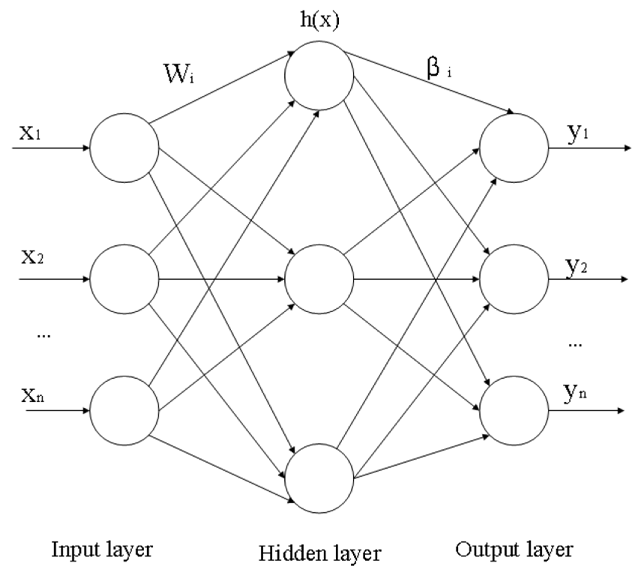
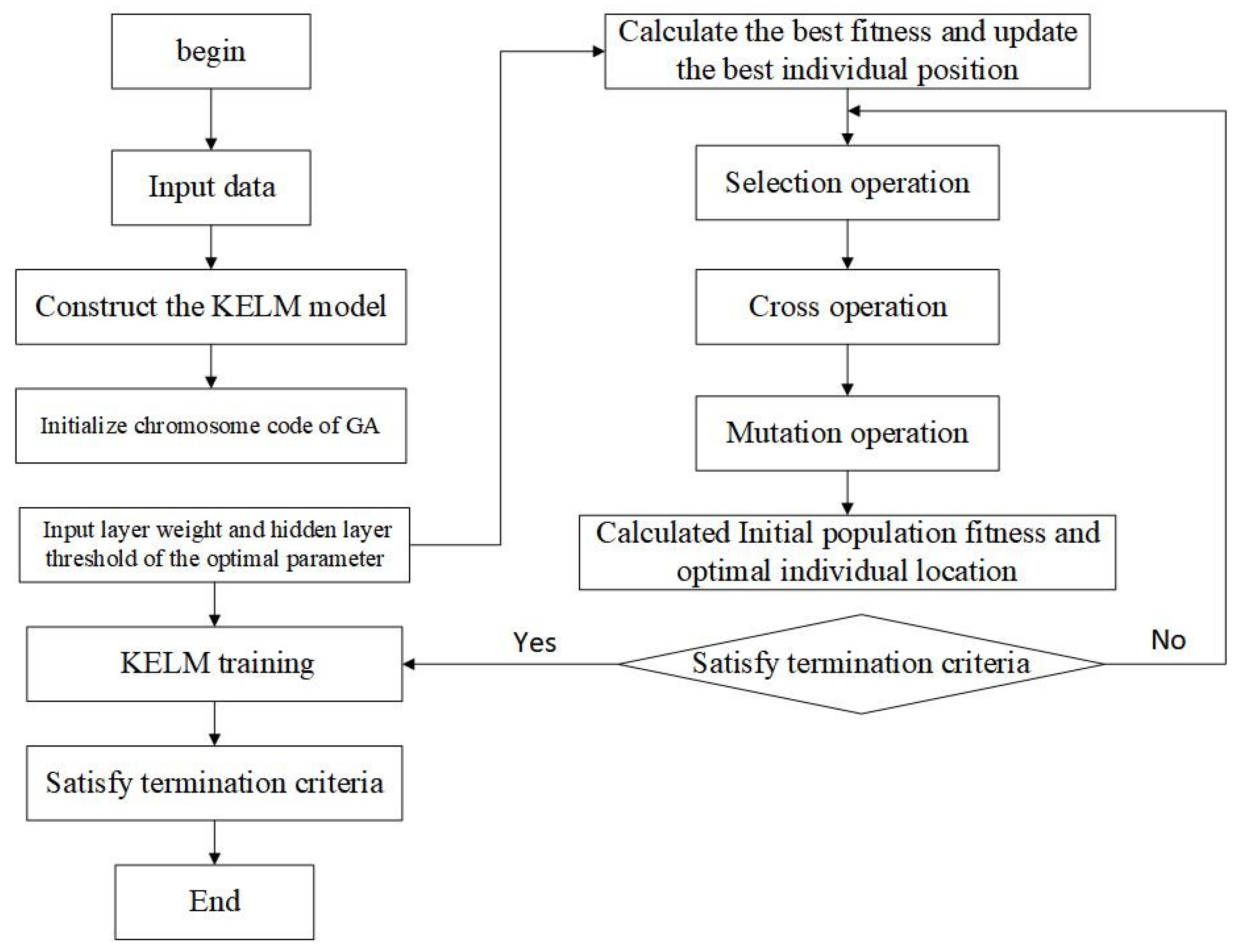
4.2. Kernel Function Extreme Learning Machine Improved by Genetic Algorithm

An extreme learning machine (ELM) is a single hidden layer feedforward artificial neural network, which has faster operation speed and better generalization performance than traditional algorithms [38]. In the training process of ELM, the connection weights of the input layer and the hidden layer are randomly generated, and the connection weights of the hidden layer and the output layer are obtained by solving the equation rather than iteratively adjusting. Better performance can be obtained only by adjusting the number of neurons in the hidden layer, which greatly enhances the learning speed. The network structure of ELM is shown in Figure 12, which consists of the input layer, hidden layer and output layer.

In the figure above, $x_n$ is the eigenvector of the input sample; $W_i$ is the connection weight of the input layer and the hidden layer; ${\beta }_i$ is the connection weight of the hidden layer and the output layer; $y_n$ is the label vector corresponding to the sample; $h\left(x\right)=\left[h_1\left(x\right),\cdots ,h_i\left(x\right)\right]$ is hidden layer output, the calculation formula of $h_i\left(x\right)$ is as follows:

$$h_i\left(x\right)=g\left(W_i,b_i,x\right)=g\left(W_{i}x+b_i\right)$$

(14)

In Equation (14), $g\left(\cdot \right)$ is the activation function; $b_i$ is the deviation of the hidden layer unit.

In an extreme learning machine, the number of hidden layer neurons needs to be determined to obtain the unique optimal solution. While the kernel function extreme learning machine (KELM) replaces the unknown hidden layer feature mapping with the kernel function, it does not need to determine the number of hidden layer nodes in advance but only obtains its kernel function. The basic principle of the kernel function is to map the input space sample data to the high-dimensional feature space by the nonlinear function, and then process the high-dimensional feature space. The key point is to transform the product operation in the high dimensional space after nonlinear transformation into the kernel function calculation in the original input space by introducing the kernel function [39]. The kernel function formula is as follows:

$${\Omega }_{i,j}=h_i\left(x\right)\cdot h_j\left(x\right)=K\left(x_i,x_j\right)$$

(15)

$$K\left(x_i,x_j\right)=\exp \left(-\frac{{‖x-x_i‖}^2}{{\delta }^2}\right)$$

(16)

In Equation (16), $K\left(x_i,x_j\right)$ is the element of the kernel matrix $\Omega$; $\delta$ is the parameter of the kernel function.

Meanwhile, the main means of the numerical solution is iterative operation, and the general iterative method is easy to fall into the local minimal loop. The genetic algorithm (GA) is a globally improved algorithm that follows the principle of survival of the fittest. It uses the “random selection according to probability” search method to avoid the trap of local optimal cleverly, and has good convergence. In order to improve the accuracy of the neural network algorithm, a kernel function extreme learning machine improved by genetic algorithm (GA-KELM) is proposed. Setting the population number to 20, the maximum number of iterations to 100, the crossover probability to 0.7, and the mutation probability to 0.3, the performance workflow of GA-KELM is shown in Figure 13.

In this algorithm, the input weights of KELM training data and the threshold of hidden layer nodes are mapped to genes on each chromosome in the GA population. The chromosome fitness of GA corresponds to the training error of KELM, and the problem of obtaining the optimal input weight and threshold is transformed into the problem of selecting the optimal chromosome by reducing the chromosome fitness. Through GA selection, crossover, mutation and other genetic operations, the optimal chromosome is selected as the input weight and threshold of KELM after being improved. The output weights of hidden layer neurons are calculated by the least squares method to calculate the predicted output. The algorithm integrates the global search ability of GA and the strong learning ability of KELM, which can effectively improve prediction accuracy.

4.3. Prediction Results and Analysis

The ELM and GA-KELM prediction models are established by MATLAB R2018a, and 100 sets of features of magnetic flux leakage signal distribution curves are selected as data sets to predict corrosion defects. Each data set comprises eight distinct parameters. Among them, P₁, P₂, A₁, A₂, W₁, W₂ and S are taken as inputs, and the defect depth and defect length are, respectively, taken as outputs. In total, 80 groups of data are randomly selected as the training set, and the remaining 20 groups of data are selected as the test set.

Figure 14 shows the comparison of prediction results of the two models. It can be seen from the figure that the accuracy of the GA-KELM model in predicting defect depth and defect length is 98.8% and 98.2%, respectively, which is 5.4% and 5.2% higher than that of the traditional ELM model. It shows that the GA-KELM model established in this paper can well predict the corrosion defect dimension, the improved algorithm adopted can effectively improve the prediction performance, and the prediction accuracy of the improved model is significantly improved.

5. Conclusions

In this paper, a calculation model of pipeline stress corrosion is established by the numerical simulation method. Furthermore, this paper analyzes the transformation law of magnetic flux leakage signal distributions. In addition, it combines improved artificial neural network algorithms to predict the corrosion defect depth and length. The following conclusions are deduced:

(1)

In this study, the accuracy of the numerical simulation results for pipeline stress corrosion is validated by published experimental data. Therefore, the effectiveness of the finite element model established herein in calculating corrosion defect changes is confirmed.

(2)

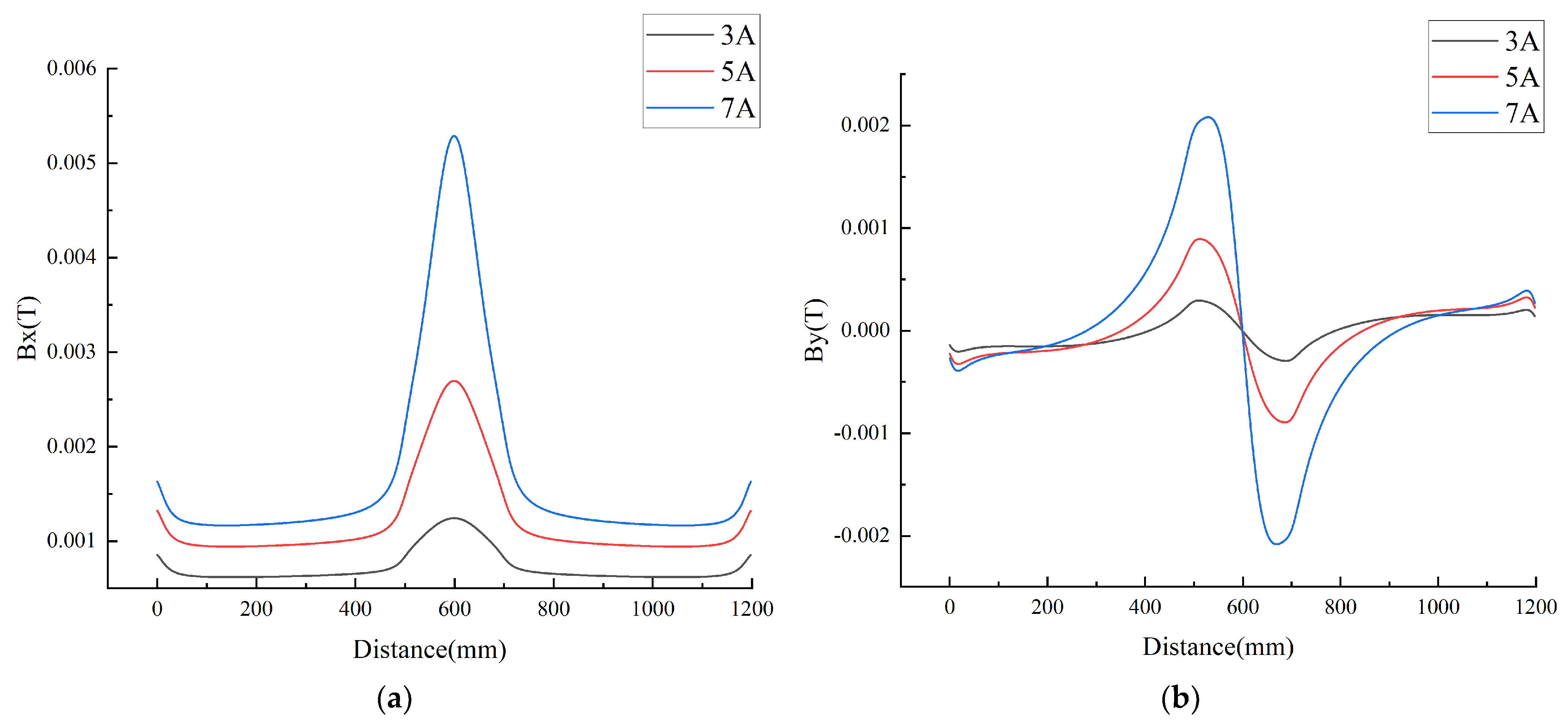
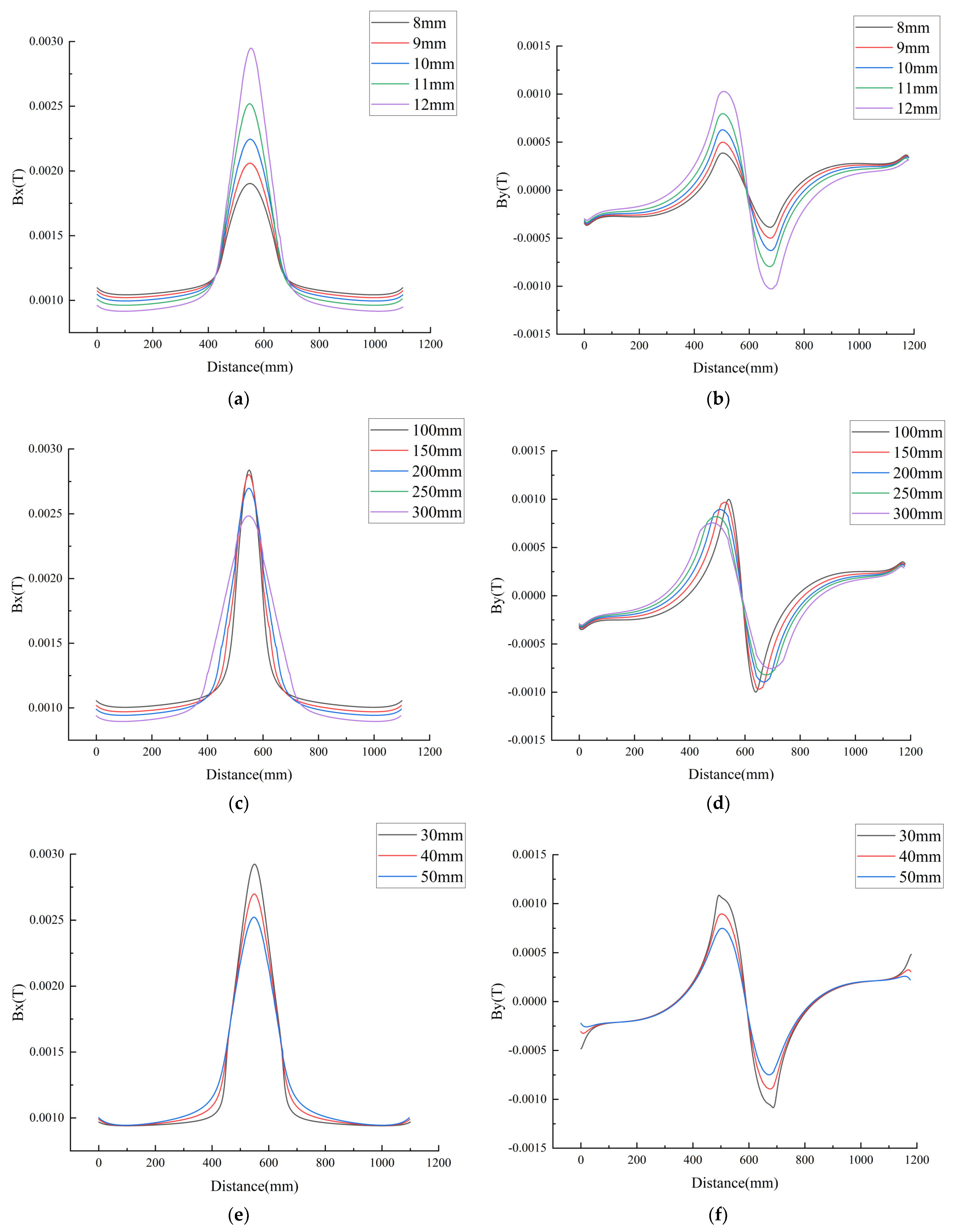
Different geometric features result in different magnetic flux leakage signal distributions. With the increase in defect depth, the area enclosed by the magnetic flux leakage signal distribution curve increases, and the extreme value of the curve also increases. As the defect length increases, the width of the curve crest increases, but the extreme value of the curve decreases. Correspondingly, a rise in lifting height corresponds to a conspicuous reduction in the curve’s extreme value.

(3)

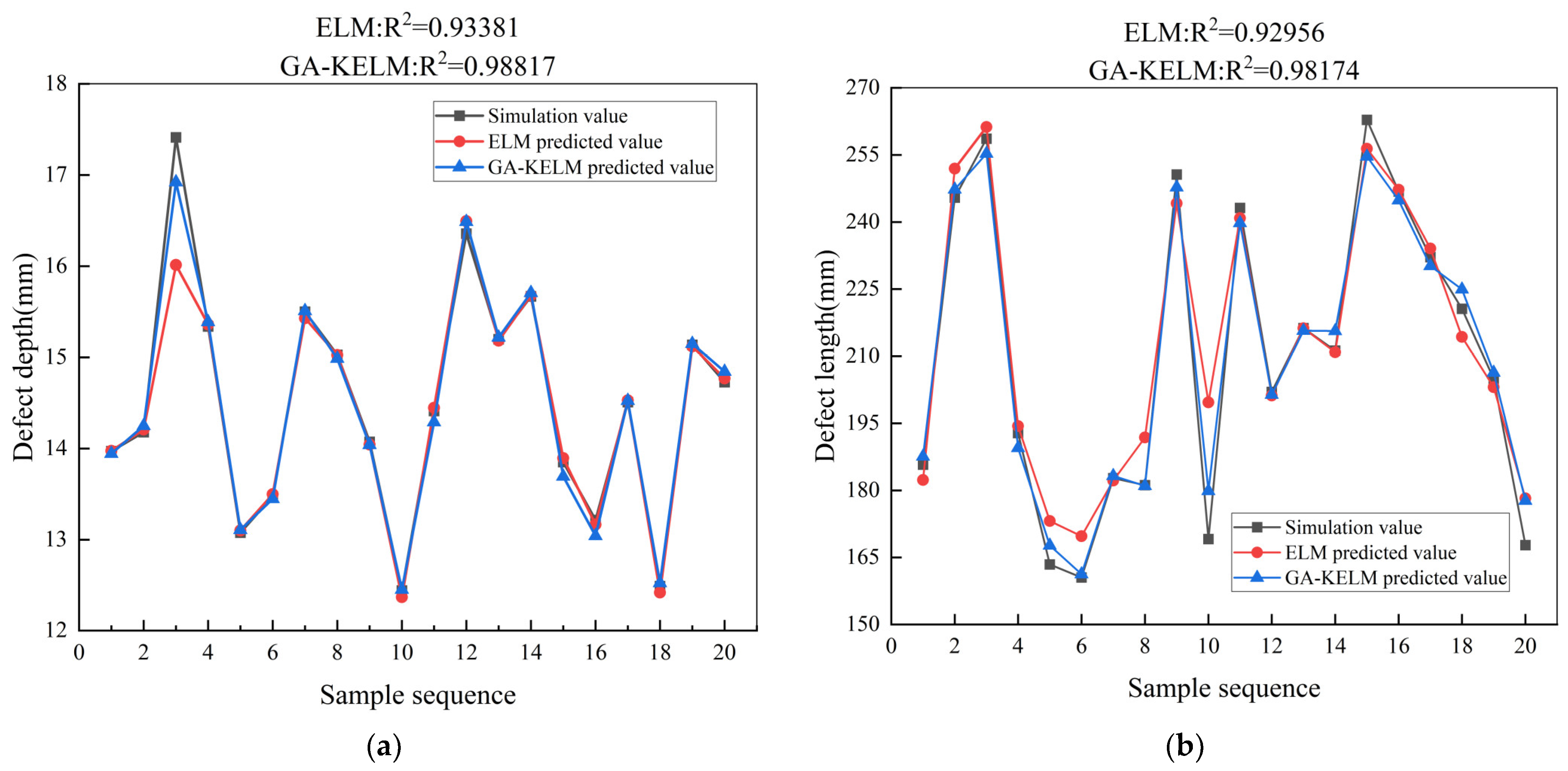
As described above, the established GA-KELM model demonstrates excellent predictive ability, accurately predicting changes in corrosion defect depth and length, with prediction accuracies of 98.8% and 98.2%, respectively, which shows improvements of 5.4% and 5.2% over the traditional ELM model.

6. Future Directions

There are still many limitations and deficiencies in the study, which need to be improved in future work:

(1)

In the present study, magnetic flux leakage testing has been explored as a method for detecting small-sized defects. However, it is crucial to acknowledge that the method becomes impractical when the defect size exceeds the coverage area of the magnetic yoke. Another noteworthy non-destructive testing approach is acoustic testing. In acoustic testing, sound signals propagate along the pipe wall, and signals carrying defect-related information can escape into the surrounding medium. Thus, the location and size of defects can be determined with appropriate acoustic equipment [40]. Importantly, acoustic inspection technology is not constrained by defect size, making it a valuable option for addressing larger defects.

(2)

Moreover, it is essential to consider the impact of various factors on the magnetic flux leakage signal, including the anti-corrosion measures applied to pipelines, the properties of pipe wall coatings, and the chemical composition of pipe material. In our future research, we will thoroughly investigate how these properties influence the outcomes of non-destructive testing.

(3)

Furthermore, the accurate determination of the defect’s location is of paramount importance. In our subsequent research endeavors, we intend to advance our methodology to enable the precise detection of both defect size and defect location, thus enhancing the comprehensiveness and effectiveness of our non-destructive testing approach.

References

1. Frank, Y.C. Stress Corrosion Cracking of Pipelines; John Wiley & Sons: Hoboken, NJ, USA, 2013; pp. 21–24. [Google Scholar]
2. Chen, W.; Boven, V.G.; Rogge, R. The role of residual stress in neutral pH stress corrosion cracking of pipeline steels—Part II: Crack dormancy. Acta Mater. 2007, 55, 43–53. [Google Scholar] [CrossRef]
3. Shahzamanian, M.M.; Meng, L.; Muntaseer, K.; Nader, Y.G.; Samer, A. Systematic literature review of the application of extended finite element method in failure prediction of pipelines. J. Pipeline Sci. Eng. 2021, 1, 241–251. [Google Scholar] [CrossRef]
4. Khalajestani, K.M.; Bahaari, M.R. Investigation of pressurized elbows containing interacting corrosion defects. Int. J. Press. Vessel. Pip. 2014, 123–124, 77–85. [Google Scholar] [CrossRef]
5. Oleksiy, L.; Kseniia, P.; Ruslan, M. Statistical estimation of residual strength and reliability of Corroded Pipeline Elbow Part based on a direct FE-simulations. J. Serbian Soc. Comput. Mech. 2018, 12, 80–95. [Google Scholar]
6. Nahal, M.; Khelif, R. A finite element model for estimating time-dependent reliability of a corroded pipeline elbow. Int. J. Struct. Integr. 2020, 12, 306–321. [Google Scholar] [CrossRef]
7. Zhang, J.; Lian, Z.; Zhou, Z.; Song, Z.; Liu, M.; Yang, K.; Liu, Z. Safety and reliability assessment of external corrosion defects assessment of buried pipelines—Soil interface: A mechanisms and FE study. J. Loss Prev. Process Ind. 2023, 82, 105006. [Google Scholar] [CrossRef]
8. Yang, Z.; Qu, P.; Li, Y.; Zhang, Z.; Gao, Y. External magnetic leakage testing of pressure pipe based on finite element analysis. Nondestruct. Test. 2021, 43, 7–12. (In Chinese) [Google Scholar]
9. Liao, X.; Wang, F.; Zhao, D.; Sun, Z.; Zhou, T. Review on Industrial Pipeline Magnetic Flux Leakage Testing Technique and Its Development Situation. Value Eng. 2016, 35, 236–237. (In Chinese) [Google Scholar]
10. Afzal, M.; Udpa, S. Advanced signal processing of magnetic flux leakage data obtained from seamless gas pipeline. NDT E Int. 2002, 35, 449–457. [Google Scholar] [CrossRef]
11. Carvalho, A.A.; Rebello, J.M.A.; Sagrilo, L.V.S.; Camerini, C.S.; Miranda, I.J.V. MFL signals and artificial neural networks applied to detection and classification of pipe weld defects. NDT E Int. 2006, 39, 661–667. [Google Scholar] [CrossRef]
12. Nestleroth, J.; Davis, J.R. Application of eddy currents induced by permanent magnets for pipeline inspection. NDT E Int. 2006, 40, 77–84. [Google Scholar] [CrossRef]
13. Joshi, A.; Udpa, L.; Udpa, S.; Tamburrino, A. Adaptive Wavelets for Characterizing Magnetic Flux Leakage Signals from Pipeline Inspection. IEEE Trans. Magn. 2006, 42, 3168–3170. [Google Scholar] [CrossRef]
14. Khodayari-Rostamabad, A.; Reilly, J.P.; Nikolova, N.K.; Hare, J.R.; Pasha, S. Machine Learning Techniques for the Analysis of Magnetic Flux Leakage Images in Pipeline Inspection. IEEE Trans. Magn. 2009, 45, 3073–3084. [Google Scholar] [CrossRef]
15. Gotoh, Y.; Sakurai, K.; Takahashi, N. Electromagnetic Inspection Method of Outer Side Defect on Small and Thick Steel Tube Using Both AC and DC Magnetic Fields. IEEE Trans. Magn. 2009, 45, 4467–4470. [Google Scholar] [CrossRef]
16. Wilson, W.J.; Kaba, M.; Tian, Y.G.; Licciardi, S. Feature extraction and integration for the quantification of PMFL data. Nondestruct. Test. Eval. 2010, 25, 661–667. [Google Scholar] [CrossRef]
17. Usarek, Z.; Warnke, K. Inspection of Gas Pipelines Using Magnetic Flux Leakage Technology. Adv. Mater. Sci. 2017, 17, 37–45. [Google Scholar] [CrossRef]
18. Machado, A.M.; Rosado, L.; Pedrosa, N.; Vostner, A.; Miranda, R.M.; Piedade, M.; Santos, G.Y. Novel eddy current probes for pipes: Application in austenitic round-in-square profiles of ITER. NDT E Int. 2017, 87, 111–118. [Google Scholar] [CrossRef]
19. Ege, Y.; Coramik, M. A new measurement system using magnetic flux leakage method in pipeline inspection. Measurement 2018, 123, 163–174. [Google Scholar] [CrossRef]
20. Makoto, T.; Masafumi, K.; Yuji, G. Examination of Inspection Method for Outer-side Defect on Ferromagnetic Steel Tube by Velocity Effect Using Insertion-type Static Magnetic Field Sensor. Sens. Mater. 2021, 33, 2867–2877. [Google Scholar]
21. Zhao, Y.; She, M.; Qiang, Y. Finite element simulation of pipe permeability at the wall defect after saturation magnetization. Oil Gas Storage Transp. 2021, 40, 539–554. (In Chinese) [Google Scholar]
22. Hu, J.; Liu, S.; Zheng, L.; Xu, Z.; Tang, J. Distinction method of pipeline inner and outer defects based on the dynamic magnetic multipole field. Oil Gas Storage Transp. 2021, 40, 673–678. (In Chinese) [Google Scholar]
23. Zheng, F.; Yang, L.; Bai, S.; Gao, S. Research on Stress Detection Method of Oil and Gas Pipeline Based on Electromagnetic Technology. Instrum. Tech. Sens. 2022, 1, 87–92. (In Chinese) [Google Scholar]
24. Feng, B.; Wu, J.; Tu, H.; Tang, J.; Kang, Y. A Review of Magnetic Flux Leakage Nondestructive Testing. Materials 2022, 15, 7362. [Google Scholar] [CrossRef]
25. Chen, Y.; Chen, B.; Yao, Y.; Tan, C.; Feng, J. A spectroscopic method based on support vector machine and artificial neural network for fiber laser welding defects detection and classification. NDT E Int. 2019, 108, 102176. [Google Scholar] [CrossRef]
26. Feng, J.; Yuan, H.; Hu, Y.; Lin, J.; Liu, S.; Luo, X. Research on deep learning method for rail surface defect detection. IET Electr. Syst. Transp. 2020, 10, 436–442. [Google Scholar] [CrossRef]
27. Arif, J.J.M.; Anwar, M.A.P.; Fakhri, A.N.A.; Zahari, T.; Edmund, Y. Evaluation of the machine learning classifier in wafer defects classification. ICT Express 2021, 7, 535–539. [Google Scholar]
28. Sun, H.; Peng, L.; Huang, S.; Li, S.; Zhao, W. Development of a Physics-Informed Doubly Fed Cross-Residual Deep Neural Network for High-Precision Magnetic Flux Leakage Defect Size Estimation. IEEE Trans. Ind. Inform. 2021, 18, 1629–1640. [Google Scholar] [CrossRef]
29. Wang, Q. Numerical Simulation of Erosion Characteristics of Oil and Gas Pipelines Containing Defects and Research on Residual Strength Prediction Technology. Master’s Thesis, Harbin University of Science and Technology, Harbin, China, 2023. (In Chinese). [Google Scholar]
30. Xu, L.; Cheng, Y. Corrosion of X100 pipeline steel under plastic strain in a neutral pH bicarbonate solution. Corros. Sci. 2012, 64, 145–152. [Google Scholar] [CrossRef]
31. Park, J.J.; Pyun, S.L.; Na, K.H.; Lee, S.M.; Kho, Y.T. Effect of Passivity of the Oxide Film on Low-pH Stress Corrosion Cracking of API 5L X-65 Pipeline Steel in Bicarbonate Solution. Corros. J. Sci. Eng. 2002, 58, 329–336. [Google Scholar] [CrossRef]
32. Bagotsky, V.S. Fundamentals of Electrochemistry, 2nd ed.; John Wiley & Sons: Hoboken, NJ, USA, 2006; pp. 23–45. [Google Scholar]
33. Gutman, E.M. Mechanochemistry of Solid Surfaces; World Scientific: Singapore, 1994; pp. 16–28. [Google Scholar]
34. Zhao, M. Corrosion and Protection of Metals; National Defense Industry Press: Beijing, China, 2008; pp. 56–58. [Google Scholar]
35. Xu, L.; Cheng, Y. Development of a finite element model for simulation and prediction of mechanoelectrochemical effect of pipeline corrosion. Corros. Sci. 2013, 73, 150–160. [Google Scholar] [CrossRef]
36. Wu, D.; Liu, Z.; Wang, X.; Su, L. Composite magnetic flux leakage detection method for pipelines using alternating magnetic field excitation. NDT E Int. 2017, 91, 148–155. [Google Scholar] [CrossRef]
37. Gao, P. Research on Pipeline Defect Detection and Recognition Method Based on Magnetic Leakage Principle. Master’s Thesis, Shenyang University of Technology, Shenyang, China, 2020. (In Chinese). [Google Scholar]
38. Tian, S.; Ma, L.; Li, H.; Tian, F.; Mao, J. Research on a Coal Seam Gas Content Prediction Method Based on an Improved Extreme Learning Machine. Appl. Sci. 2023, 13, 8753. [Google Scholar] [CrossRef]
39. Zhang, Q.; Tsang Eric, C.C.; He, Q.; Guo, Y. Ensemble of kernel extreme learning machine based elimination optimization for multi-label classification. Knowl.-Based Syst. 2023, 278, 110817. [Google Scholar] [CrossRef]
40. Qian, X. Acoustic Detection of Gas-Liquid Mixing Pipeline and Research on Safety Operation. Master’s Thesis, China University of Petroleum (East China), Qingdao, China, 2010. (In Chinese). [Google Scholar]
Figure 1. Stress–strain curve of X100 pipeline steel.
Electronics 12 03707 g001
Figure 2. Calculation model of pipeline stress corrosion.
Electronics 12 03707 g002
Figure 3. Corrosion potential change with von Mises stress of X100 pipeline steel.
Electronics 12 03707 g003
Figure 4. Variation of defect dimension with corrosion time.
Electronics 12 03707 g004
Figure 5. Refraction of magnetic induction line.
Electronics 12 03707 g005
Figure 6. Principle of magnetic flux leakage testing.
Electronics 12 03707 g006
Figure 7. Calculation model of magnetic flux leakage testing.
Electronics 12 03707 g007
Figure 8. B-H curve of X100 pipeline steel.
Electronics 12 03707 g008
Figure 9. Distribution of magnetic flux leakage signal under different parameter conditions. (a) Axial component of current value signal with 500 turns. (b) Radial component of current value signal with 500 turns. (c) Axial component of coils’ number signal with 5A current. (d) Radial component of coils’ number signal with 5A current.
Electronics 12 03707 g009aElectronics 12 03707 g009b
Figure 10. Distribution of magnetic flux leakage signal under different geometric characteristics. (a) Axial component of defect depth signal. (b) Radial component of defect depth signal. (c) Axial component of defect length signal. (d) Radial component of defect length signal. (e) Axial component of lifting height signal. (f) Radial component of lifting height signal.
Electronics 12 03707 g010
Figure 11. Feature of the curve. (a) Axial component. (b) Radial component.
Electronics 12 03707 g011
Figure 12. ELM network structure.
Electronics 12 03707 g012
Figure 13. GA-KELM perform workflow.
Electronics 12 03707 g013
Figure 14. Comparison of prediction results. (a) Schematic diagram of defect depth. (b) Schematic diagram of defect length.
Electronics 12 03707 g014