A Robust Interval Optimization Method for Combined Heat and Power Dispatch

Abstract

The increasing penetration of renewable energy, particularly wind power, and the integration of different energy systems have become two major trends in the development of energy systems. In this context, this paper proposes a robust interval optimization method for combined heat and power dispatch (CHPD) to address the challenges associated with wind power accommodation. To enhance the flexibility of a power system and support the integration of wind power, flexibility resources from a district heating system are introduced in the economic dispatch. To ensure the safety and reliability of the CHPD results, a robust interval optimization method is employed. By considering a range of possible wind power outputs, the robust interval optimization method provides a robust and reliable dispatch plan that can accommodate uncertainties and fluctuations in wind power generation. To verify the effectiveness of the proposed model and method, case studies were conducted on a 6-bus electrical power system connected with a 6-node district heating system. The results demonstrate that the proposed approach can effectively enhance the integration of wind power and improve the overall reliability and flexibility of the energy system.

1. Introduction

In recent years, there has been a growing demand for a cleaner and more sustainable energy system. This shift in global energy priorities has led to the rapid growth of wind power as one of the key sources of renewable energy. Wind power has the ability to harness the natural power of wind and convert it into electricity, making it an attractive option for reducing greenhouse gas emissions and transitioning to a cleaner power system.

However, the integration of wind power into the existing power grid presents certain challenges. One of the main challenges is the random and fluctuating nature of wind power output. Unlike traditional power plants, which have a steady and predictable output, wind turbines are highly dependent on weather conditions and can vary in their output from one moment to the next. This poses a serious risk to the reliable operation of power systems, as the sudden changes in wind power output can destabilize the grid and lead to power outages.

To address this issue, researchers have been exploring the coordinated operation of an electrical power system (EPS) and district heating systems (DHSs) as a means of increasing the flexibility of a power system and mitigating the operational risks caused by wind power uncertainty. By coupling an EPS and DHSs through combined heat and power dispatch (CHPD), which involves the use of CHP units, boilers, pumps, and other components, it is possible to optimize the operation of a system and enhance its ability to accommodate wind power fluctuations.

Researchers have conducted numerous studies on combined heat and power dispatch (CHPD). Ref. [1] first proposed the CHPD concept, optimized the operational cost, and enhanced the wind power consumption capacity of a system by using the pipeline heat storage capacity. Ref. [2] analyzed the impact of boilers and heat pumps on wind penetration. Refs. [3,4] simulated the phase change process of heat storage, and introduced the CHP engine heat transfer process into CHPD. Ref. [5] introduced electric boilers with heat storage tanks in CHPD and found that they facilitate wind power accommodation. Refs. [6,7,8,9,10] investigated the thermal inertia of buildings and their power load shifting capacity. These studies have focused on optimizing the operational costs and enhancing the wind power consumption capacity of systems by using boilers, heat pumps, and the thermal inertia of buildings.

However, most of these studies have treated the CHPD problem as a deterministic one, without directly considering the uncertainty of wind power output. This means that the reliability of EPS operation cannot be guaranteed, and the results obtained are likely to be infeasible even for small wind power output perturbations. Specifically, the results may violate the power system reserve capacity limit or line transmission capacity limit. Thus, a “safe” CHPD method is required to cope with the wind power output uncertainty.

To address this limitation, researchers have started exploring stochastic optimization and chance-constrained optimization techniques to account for wind power output uncertainty in CHPD [7,11]. However, these approaches have their own limitations, such as the computational difficulty of stochastic optimization and the need for a priori knowledge of the probability distribution of uncertain parameters.

In recent years, robust optimization (RO) has emerged as a promising approach for dealing with uncertainty in CHPD. Unlike stochastic optimization and chance-constrained optimization, RO does not require explicit knowledge of the probability distribution of uncertain parameters. Instead, it focuses on finding solutions that are robust against a range of possible scenarios. Ref. [11] proposed a robust combined heat and power dispatch (R-CHPD) model that considers demand response uncertainty. Ref. [12] proposed a robust short-term CHPD scheme. Ref. [13] proposed a data-driven R-CHPD model solved by the C&CG algorithm.

However, the existing R-CHPD is formulated with a min–max or max–min objective function, which assumes that wind power can be fully absorbed even under extreme and unstable wind power conditions. In reality, wind curtailment is sometimes necessary to ensure the stability and reliability of the power system, especially during periods of low load demand. To address this issue, this paper proposes a novel robust CHPD framework that takes into account the uncertainty of wind power output and allows for wind curtailment when necessary. The proposed framework utilizes a robust interval approach, where the predicted wind output intervals are uploaded to the dispatch center. The CHPD problem is then optimized to calculate the allowable wind output within these intervals. The allowable interval is sent back to the wind farms as their control target, and CHPD for thermal units is applied accordingly. This approach ensures that the power system operates within safe limits and can effectively handle the uncertainty of wind power output.

To demonstrate the effectiveness of the proposed framework, numerical simulations are conducted in a case study. The results show that the proposed method significantly improves the reliability and stability of the power system, even under uncertain wind power conditions. The flexibility provided by the coordinated operation of the EPS and DHSs through CHPD allows for better integration of wind power and increases the overall efficiency of the system.

The paper is organized as follows. In Section 2, the paper provides a deterministic model of CHPD. This model aims to optimize the dispatch of both heat and power generation units in a system. It takes into account various constraints such as energy demand, fuel cost, and operational limitations of the units. Moving on to Section 3, a robust interval model of CHPD is presented along with its corresponding solution method. This model considers uncertainties and variations in input parameters to account for real-world scenarios where exact values are not always available. In addition, the solution method proposed in Section 3 effectively handles the interval constraints and provides practical solutions. To evaluate the performance and effectiveness of the proposed models, Section 4 presents a series of numerical simulations. The results obtained from the simulations are analyzed and compared to demonstrate the advantages and limitations of each model. Finally, in Section 5, the conclusion of the paper is provided. This section summarizes the key findings and contributions of the research. It also discusses the implications of the results and suggests potential directions for future work.

2. Deterministic Model of CHPD

2.1. Objective Function

In order to optimize the operation of units, the objective function of CHPD is designed to minimize the total operational cost. This cost is modeled as a quadratic equation, taking into account various factors that contribute to the overall cost. First, the fuel cost of non-CHP units ${\sum }_{t\in {\rm T}}{C}_t^G$ is considered in the objective function. These units are responsible for generating electricity without the simultaneous production of heat. The cost of fuel consumed by these units directly impacts the overall operation cost and therefore needs to be minimized. Second, the penalty cost of wind curtailment ${\sum }_{t\in {\rm T}}{C}_t^W$ is also included in the objective function. Wind power generation is inherently uncertain due to the variability and intermittency of wind resources. In situations where the wind power output exceeds the demand or the capacity of the power grid, curtailment is necessary to maintain grid stability. However, curtailment leads to a loss in potential renewable energy generation and thus incurs a penalty cost. By considering this penalty cost, the objective function aims to optimize the use of wind power while minimizing curtailment. Third, the fuel cost of CHP units ${\sum }_{t\in {\rm T}}{C}_t^{CHP}$ is accounted for in the objective function. CHP units generate both electricity and heat simultaneously, making them more efficient compared to the separate generation of electricity and heat. The fuel cost associated with operating these CHP units is an important component of the total operational cost and needs to be minimized.

$$min{\sum }_{t\in {\rm T}}{C}_t^G+{\sum }_{t\in {\rm T}}{C}_t^W+{\sum }_{t\in {\rm T}}{C}_t^{CHP}$$

(1)

$$C_{i,t}^G=a_{0,i}^G+a_{1,i}^G{P}_{i,t}^G+a_{2,i}^G{(P_{i,t}^G)}^2,\forall i\in {\Omega }_G,\forall t\in {\rm T}$$

(2)

$$C_{i,t}^W={\sigma }_{}^W{({\overline{P}}_i^W-P_{i,t}^W)}^2,\forall i\in {\Omega }_W,\forall t\in {\rm T}$$

(3)

$$\begin{array}{c}{C}_{i,t}^{CHP}=a_{0,i}^{CHP}+a_{1,i}^{CHP}{P}_{i,t}^{CHP}+a_{2,i}^{CHP}{H}_{i,t}^{CHP}+a_{3,i}^{CHP}{P}_{i,t}^{CHP}\\ \hfill \hspace{1em}\hspace{1em}\hspace{1em}\hspace{1em}+a_{4,i}^{CHP}{(P_{i,t}^{CHP})}^2+a_{5,i}^{CHP}{(H_{i,t}^{CHP})}^2,\forall i\in {\Omega }_{CHP},\forall t\in {\rm T}\end{array}$$

(4)

where $P_{i,t}^G$ is the variable for the power output of non-CHP unit i at period t. $P_{i,t}^W$ is the variable for the power output of wind farm i during period t. $P_{i,t}^{CHP}$ and $H_{i,t}^{CHP}$ are variables for the power and heat output of CHP units i during period t, respectively. ${\Omega }_G$, ${\Omega }_W$, and ${\Omega }_{CHP}$ are sets for non-CHP units, wind farms, and CHP units, respectively. $a_{0,i}^G$, $a_{1,i}^G$, and $a_{2,i}^G$ are cost coefficients of non-CHP i. $a_{0,i}^{CHP}$, $a_{1,i}^{CHP}$, $a_{2,i}^{CHP}$, $a_{3,i}^{CHP}$, $a_{4,i}^{CHP}$, and $a_{5,i}^{CHP}$ are the cost coefficients of CHP i. ${\sigma }_{}^W$ is the penalty factor of wind curtailment.

2.2. DHS Constraints

Heat stations are the primary sources of heat in a DHS. The heat generated in the heat stations is transferred to the heat loads through a network of pipelines. These pipelines are designed to transport hot water or steam to various buildings and facilities within the district. The circulating water in the pipelines acts as a medium to transfer the heat from the heat stations to the heat loads. In this part, the heat stations, pipelines, and heat loads are formulated as given below.

2.2.1. Heat Station

In addition to CHP units, there are other heat sources commonly utilized in heat stations such as heating boilers and heat tanks. However, for the sake of simplicity, this discussion will focus solely on the use of CHP units as heat sources.

In engineering practice, there are two commonly employed types of CHP units: back-pressure turbines and extraction-condensing turbines. These units play a crucial role in generating heat for various applications. In order to accurately model the outputs of these CHP units, it is common practice to use convex combinations of the operational region poles [14]. By considering the different operating conditions and parameters, engineers can develop mathematical models that accurately represent the performance of these units. This modeling approach allows for better control and optimization of the CHP system, leading to improved efficiency and overall performance.

$$P_{i,t}^{CHP}={\sum }_{j\in O{R}^i}{\lambda }_{i,t,j}{p}_{i,j}^{CHP},H_{i,t}^{CHP}={\sum }_{j\in O{R}^i}{\lambda }_{i,t,j}{h}_{i,j}^{CHP},\forall t\in {\rm T},\forall i\in {\Omega }_{CHP}$$

(5)

$$0\le {\lambda }_{i,t,j}^{CHP}\le 1,{\sum }_{j\in O{R}^i}{\lambda }_{i,t,j}^{CHP}=1,\forall j\in O{R}^i,\forall t\in {\rm T},\forall i\in {\Omega }_{CHP}$$

(6)

where $p_{i,j}^{CHP}$ and $h_{i,j}^{CHP}$ are parameters for the power and heat output at the j-th extreme point in the operating region of CHP units i. ${\lambda }_{i,t,j}$ is variable for the operating point of CHP units i during period t. $O{R}^i$ is a set of extreme points in the operating region of CHP units i. The heat output of CHP units is utilized for heating water:

$$H_{i,t}^{CHP}=c{m}_j^{HS}\left(T_{n,t}^{NS}-T_{n,t}^{NR}\right),\forall i\in {\Omega }_{CHP},\forall j\in {\Omega }_{HS},\forall n=N_j^{HS},\forall t\in {\rm T}$$

(7)

where $c$ is a parameter for the specific thermal capacity of water. $m_j^{HS}$ is a parameter for mass flow at heat station j. $T_{n,t}^{NS}$ and $T_{n,t}^{NR}$ are variables for the water temperature in supply and return pipes at node n during period t. ${\Omega }_{HS}$ is a set of heat stations. $N_j^{HS}$ is an index of heat nodes connecting to heat station j.

2.2.2. District Heating Network

In the model of a DHN, temperature mixing Equations (8) and (9) are used to describe the process of mixing hot water from different sources. These equations take into account the flow rates and temperatures of the incoming water streams, as well as the mixed node temperature.

$${\sum }_{j\in {\Omega }_{P+}}{m}_j^{PS}{T}_{n,t}^{NS}={\sum }_{j\in {\Omega }_{P-}}\left(m_j^{PS}\cdot T_{j,t}^{PS,out}\right),\forall n\in {\Omega }_{ND},\forall t\in {\rm T}$$

(8)

$${\sum }_{j\in {\Omega }_{P+}}{m}_j^{PR}{T}_{n,t}^{NR}={\sum }_{j\in {\Omega }_{P-}}\left(m_j^{PR}\cdot T_{j,t}^{PR,out}\right),\forall n\in {\Omega }_{ND},\forall t\in {\rm T}$$

(9)

where $T_{j,t}^{PS,out}$ and $T_{j,t}^{PR,out}$ are variables representing the outflow temperatures of supply and return pipes j during period t, respectively. ${\Omega }_{ND}$ is a set of heat nodes. The heat loss Equations (10)–(14) are included in the model to account for the energy losses that occur during the transportation of hot water through the pipes of the DHN. These equations consider factors such as the insulation properties of the pipes, the ambient temperature, and the length and diameter of the pipes.

$$T_{j,t}^{PS,out\ast }=\left(1-\lceil {\varphi }_j^{PS}\rceil +{\varphi }_j^{PS}\right)T_{j,t-\lceil {\varphi }_j^{PS}\rceil }^{PS,in}+\left(\lceil {\varphi }_j^{PS}\rceil -{\varphi }_j^{PS}\right)T_{j,t-\lceil {\varphi }_j^{PS}\rceil +1}^{PS,in},\forall j\in {\Omega }_n^P,\forall t\in {\rm T}$$

(10)

$$T_{j,t}^{PS,out\ast }=\left(1-\lceil {\varphi }_j^{PR}\rceil +{\varphi }_j^{PR}\right)T_{j,t-\lceil {\varphi }_j^{PR}\rceil }^{PR,in}+\left(\lceil {\varphi }_j^{PR}\rceil -{\varphi }_j^{PR}\right)T_{j,t-\lceil {\varphi }_j^{PR}\rceil +1}^{PR,in},\forall j\in {\Omega }_n^P,\forall t\in {\rm T}$$

(11)

$$T_{j,t}^{PS,out}=T_t^{AM}+\left(T_{j,t}^{PS,out\ast }-T_t^{AM}\right)\cdot exp\left[-\frac{{\lambda }_j}{A_j\rho c}\left(\lceil {\varphi }_j^{PS}\rceil -0.5\right)\right],\forall j\in {\Omega }_n^P,\forall t\in {\rm T}$$

(12)

$$T_{j,t}^{PR,out}=T_t^{AM}+\left(T_{j,t}^{PR,out\ast }-T_t^{AM}\right)\cdot exp\left[-\frac{{\lambda }_j}{A_j\rho c}\left(\lceil {\varphi }_j^{PR}\rceil -0.5\right)\right],\forall j\in {\Omega }_n^P,\forall t\in {\rm T}$$

(13)

$${\varphi }_j^{PS}=\frac{\rho A_j{L}_j}{m_j^{PS}},{\varphi }_j^{PR}=\frac{\rho A_j{L}_j}{m_j^{PR}},\forall j\in {\Omega }_n^P,\forall t\in {\rm T}$$

(14)

where $T_{j,t}^{PS,in}$ and $T_{j,t}^{PR,in}$ are variables representing the inflow temperatures of supply and return pipes j during period t, respectively. $T_{j,t}^{PS,out\ast }$ and $T_{j,t}^{PR,out\ast }$ are the auxiliary variables indicating the pipe outlet temperature ignoring the heat loss of the pipe. ${\Omega }_n^P$ is a set of pipelines connecting with node n. ${\Omega }_n^{P+}$ and ${\Omega }_n^{P-}$ are sets of pipelines starting and ending at node n, respectively. $T_t^{AM}$ is a parameter of ambient temperature at period t. ${\varphi }_j^{PS}$ and ${\varphi }_j^{PR}$ are the water transfer times in supply and return pipelines j. ${\lambda }_j$, $L_j$, and $A_j$ are parameters for heat transfer, length, and cross-sectional area of pipe j, respectively. $\rho$ is the parameter for water density. The symbol ⌈ ⌉ is rounded up. To calculate the inlet temperature at each node in the DHN, Equations (15) and (16) are utilized.

$$T_{n,t}^{NR}=T_{j,t}^{PR,in},\forall n\in {\Omega }_{ND},\forall j={\Omega }_n^{P+},\forall t\in {\rm T}$$

(15)

$$T_{n,t}^{NS}=T_{j,t}^{PS,in},\forall n\in {\Omega }_{ND},\forall j={\Omega }_n^{P-},\forall t\in {\rm T}$$

(16)

2.2.3. Heat Loads

The heat load is presented as

$$H_{i,t}^{LD}=c{m}_i^{LD}\left(T_{n,t}^{NS}-T_{n,t}^{NR}\right),\forall i\in {\Omega }_{LD},\forall n=N_i^{LD},\forall t\in {\rm T}$$

(17)

where $H_{i,t}^{LD}$ is the variable for heat load i at period t. $m_i^{LD}$ is the parameter for the mass flow of heat load i. ${\Omega }_{LD}$ is a set of heat loads. $N_i^{LD}$ is an index of heat nodes linked to heat load j. To guarantee the heating demand, the temperature of the heat load is satisfied:

$${\underset{¯}{T}}_n^{NR}\le T_{n,t}^{NR}\le {\overline{T}}_n^{NR},\forall i\in {\Omega }_{LD},\forall n=N_i^{LD},\forall t\in {\rm T}$$

(18)

where ${\underset{¯}{T}}_n^{NR}$ and ${\overline{T}}_n^{NR}$ are the water temperature boundaries at node n.

2.3. EPS Constraints

Here, the DC model is used for EPS. The power balance constraints (19) ensure that the total power generation in the EPS matches the total power demand. This constraint is essential for maintaining system stability and avoiding power shortages or overloads. Transmission capacity constraints (20) are imposed to limit the amount of power that can flow through the transmission lines. These constraints take into account the capacity limitations of the transmission infrastructure and prevent congestion or overloading. The thermal unit ramping constraints (21) and (22) specify the rate at which thermal units can change their generation output. These constraints ensure that the units’ output changes smoothly and gradually, preventing sudden and drastic changes that could destabilize the system. The thermal units’ generation output constraints (23) and (24) define the range within which the generation output of thermal units must lie. These constraints are based on the characteristics and limitations of each thermal unit, such as its maximum and minimum output levels. Wind farms’ power output constraints (25) are used to limit the power output of wind farms. Since wind power is intermittent and dependent on weather conditions, these constraints ensure that the wind farms’ output remains within certain bounds, preventing excessive reliance on unreliable wind power. Finally, the spinning reserve constraints (26)–(28) are imposed to ensure that there is sufficient reserve capacity in the system to handle unexpected changes in demand or generation. In this study, the spinning reserve is assumed to be provided by non-CHP units, as the spinning reserve ability of CHP units is limited by their heat loads.

$${\sum }_{i\in {\Omega }_G}{P}_{i,t}^G+{\sum }_{i\in {\Omega }_{CHP}}{P}_{i,t}^{CHP}+{\sum }_{i\in {\Omega }_W}{P}_{i,t}^W={\sum }_{i\in {\Omega }_{bus}}{P}_{i,t}^{LD},\forall t\in {\rm T}$$

(19)

$$\left|{\sum }_{j\in {\Omega }_{bus}}S{F}_{l,j}\left({\sum }_{i\in S_j^G}{P}_{i,t}^G+{\sum }_{i\in S_j^{CHP}}{P}_{i,t}^{CHP}+{\sum }_{i\in S_j^W}{P}_{i,t}^W-P_{j,t}^{LD}\right)\right|\le F_l,\forall l\in {\Omega }_{line},\forall t\in {\rm T}$$

(20)

$$-R{D}_i\cdot \Delta t\le P_{i,t}^G-P_{i,t-1}^G\le -R{U}_i\cdot \Delta t,\forall i\in {\Omega }_G,\forall t\in {\rm T}$$

(21)

$$-R{D}_i\cdot \Delta t\le P_{i,t}^{CHP}-P_{i,t-1}^{CHP}\le -R{U}_i\cdot \Delta t,\forall i\in {\Omega }_{CHP},\forall t\in {\rm T}$$

(22)

$${\underset{¯}{P}}_i^G\le P_{i,t}^G\le {\overline{P}}_i^G,\forall i\in {\Omega }_G,\forall t\in {\rm T}$$

(23)

$${\underset{¯}{P}}_i^{CHP}\le P_{i,t}^{CHP}\le {\overline{P}}_i^{CHP},\forall i\in {\Omega }_{CHP},\forall t\in {\rm T}$$

(24)

$$0\le P_{i,t}^W\le {\overline{P}}_i^W,\forall i\in {\Omega }_W,\forall t\in {\rm T}$$

(25)

$$0\le r{u}_{i,t}\le R{U}_i,r{u}_{i,t}\le {\overline{P}}_i^G-P_{i,t}^G,\forall i\in {\Omega }_G,\forall t\in {\rm T}$$

(26)

$$0\le r{d}_{i,t}\le R{D}_i,r{d}_{i,t}\le P_{i,t}^G-{\underset{¯}{P}}_i^G,\forall i\in {\Omega }_G,\forall t\in {\rm T}$$

(27)

$${\sum }_{i\in {\Omega }_G}r{u}_{i,t}\ge SU,{\sum }_{i\in {\Omega }_G}r{d}_{i,t}\ge SD,\forall t\in {\rm T}$$

(28)

where $r{u}_{i,t}$ and $r{d}_{i,t}$ are variables for the upward and downward spinning reserve of non-CHP unit i at period t. $S{F}_{i,j}$ is the shift factor of bus j to line l. $F_l$ is the maximum transmission flow of line l. $R{U}_i$ and $R{D}_i$ are parameters for the upward ramping capacity and downward ramping capacity of units i, respectively. $P_{i,t}^{LD}$ is a parameter for electric load connecting to bus i during period t. ${\underset{¯}{P}}_i^G$ and ${\overline{P}}_i^G$ are parameters for the power output boundaries of non-CHP unit i, respectively. ${\underset{¯}{P}}_i^{CHP}$ and ${\overline{P}}_i^{CHP}$ are parameters for the power output boundaries of CHP unit i. ${\overline{P}}_i^W$ is a parameter for the forecast output of wind farm i. $SU$ and $SD$ are parameters for system-wide upward and downward ramping capacity. ${\Omega }_{bus}$ and ${\Omega }_{line}$ are sets for bus and line, respectively. $S_j^G$, $S_j^{CHP}$, and $S_j^W$ are sets for non-CHP units, CHP units, and wind farms connected with bus j, respectively.

3. Robust Model of CHPD and the Solution Method

Considering that the CHPD model proposed in Section 2 is unable to capture wind power uncertainty, this section first proposes a robust CHPD model, and then the robust interval optimization method is used to handle the R-CHPD problem.

3.1. Formulation of Robust CHPD

In the R-CHPD framework, the uncertain nature of wind power output is taken into account by representing it as an interval $\left[{\underset{¯}{p}}_{i,t}^W,{\overline{p}}_{i,t}^W\right]$ rather than a single value ${\overline{P}}_{i,t}^W$. This interval captures the potential range of wind power generation, considering both the lower bound ${\underset{¯}{p}}_{i,t}^W$ and upper bound ${\overline{p}}_{i,t}^W$. By considering this range, operators can analyze the worst-case scenarios and develop robust strategies to ensure the system’s safe and reliable operation. Typically, there are four worst-case scenarios, as follows:

• The worst-case scenario for the upward-spinning reserve constraint is

$$R_t^U=\left\{\begin{array}{c}\underset{P_{i,t}^W}{\min }\left({\sum }_{i\in {\Omega }_G}{P}_{i,t}^G+{\sum }_{i\in {\Omega }_{CHP}}{P}_{i,t}^{CHP}+{\sum }_{i\in {\Omega }_W}{P}_{i,t}^W+{\sum }_{i\in {\Omega }_G}r{u}_{i,t}-{\sum }_{i\in {\Omega }_{bus}}{P}_{i,t}^{LD}\right)\ge 0\hfill \\ s.t.{\widetilde{\underset{¯}{p}}}_{i,t}^W\le P_{i,t}^W\le {\overline{\tilde{p}}}_{i,t}^W,\forall i\in {\Omega }_W,\forall t\in {\rm T}\hfill \end{array}\right\}$$

(29)

where ${\widetilde{\underset{¯}{p}}}_{i,t}^W$ and ${\overline{\tilde{p}}}_{i,t}^W$ are the decision variables in a robust interval optimization problem which satisfies

$${\widetilde{\underset{¯}{p}}}_{i,t}^W\le {\underset{¯}{p}}_{i,t}^W,{\overline{\tilde{p}}}_{i,t}^W\le {\overline{p}}_{i,t}^W,\forall i\in {\Omega }_W,\forall t\in {\rm T}$$

(30)

In this scenario, the system must be prepared for the maximum amount of wind power generation, which would require a surplus of resources that can be quickly dispatched to balance the excess power.

2.

The worst-case scenario for the downward spinning reserve constraint is

$$R_t^D=\left\{\begin{array}{c}\underset{P_{i,t}^W}{\min }\left({\sum }_{i\in {\Omega }_{bus}}{P}_{i,t}^{LD}-{\sum }_{i\in {\Omega }_G}{P}_{i,t}^G-{\sum }_{i\in {\Omega }_{CHP}}{P}_{i,t}^{CHP}-{\sum }_{i\in {\Omega }_W}{P}_{i,t}^W-{\sum }_{i\in {\Omega }_G}r{d}_{i,t}\right)\ge 0\hfill \\ s.t.{\widetilde{\underset{¯}{p}}}_{i,t}^W\le P_{i,t}^W\le {\overline{\tilde{p}}}_{i,t}^W,\forall i\in {\Omega }_W,\forall t\in {\rm T}\hfill \end{array}\right\}$$

(31)

For these worst-case scenarios, the total upward power adjustment $\Delta r{u}_t$ and downward upward power adjustment $\Delta r{d}_t$ are calculated as

$$\Delta r{u}_t={\sum }_{i\in {\Omega }_G}r{u}_{i,t}-R_t^U,\Delta r{d}_t={\sum }_{i\in {\Omega }_G}r{d}_{i,t}-R_t^D,\forall t\in {\rm T}$$

(32)

$$\Delta r{u}_t={\sum }_{i\in {\Omega }_G}\Delta r{u}_{i,t},\Delta r{d}_t={\sum }_{i\in {\Omega }_G}\Delta r{d}_{i,t},\forall t\in {\rm T}$$

(33)

$\Delta r{u}_t$ and $\Delta r{d}_t$ should be shared by all the non-CHP units, so the following constraints exist:

$$0\le \Delta r{u}_{i,t}\le r{u}_{i,t},0\le \Delta r{d}_{i,t}\le r{d}_{i,t},i\in {\Omega }_G,\forall t\in {\rm T}$$

(34)

$$P_{i,t}^G+\Delta r{u}_{i,t}-P_{i,t-1}^G+\Delta r{d}_{i,t-1}\le \Delta P{U}_{i,t}^G,i\in {\Omega }_G,\forall t\in {\rm T}$$

(35)

$$P_{i,t-1}^G+\Delta r{u}_{i,t-1}-P_{i,t}^G+\Delta r{d}_{i,t}\le \Delta P{D}_{i,t}^G,i\in {\Omega }_G,\forall t\in {\rm T}$$

(36)

3.

The worst-case scenario for the positive transmission interface flow constraint is

$$L_{l,t}^U=\left\{\begin{array}{c}\underset{P_{i,t}^W}{\max }\left({\sum }_{j\in {\Omega }_{bus}}S{F}_{l,j}\left({\sum }_{i\in S_j^G}{P}_{i,t}^G+{\sum }_{i\in S_j^{CHP}}{P}_{i,t}^{CHP}+{\sum }_{i\in S_j^W}{P}_{i,t}^W-P_{j,t}^{LD}\right)\right)\le F_l\hfill \\ s.t.{\widetilde{\underset{¯}{p}}}_{i,t}^W\le P_{i,t}^W\le {\overline{\tilde{p}}}_{i,t}^W,\forall i\in {\Omega }_W,\forall l\in {\Omega }_{line}, \forall t\in {\rm T}\hfill \end{array}\right\}$$

(37)

4.

The worst-case scenario for the negative transmission interface flow constraint is

$$L_{l,t}^D=\left\{\begin{array}{c}\underset{P_{i,t}^W}{\min }\left({\sum }_{j\in {\Omega }_{bus}}S{F}_{l,j}\left({\sum }_{i\in S_j^G}{P}_{i,t}^G+{\sum }_{i\in S_j^{CHP}}{P}_{i,t}^{CHP}+{\sum }_{i\in S_j^W}{P}_{i,t}^W-P_{j,t}^{LD}\right)\right)\ge -F_l\hfill \\ s.t.{\widetilde{\underset{¯}{p}}}_{i,t}^W\le P_{i,t}^W\le {\overline{\tilde{p}}}_{i,t}^W,\forall i\in {\Omega }_W,\forall l\in {\Omega }_{line},\forall t\in {\rm T}\hfill \end{array}\right\}$$

(38)

Moreover, the penalty cost function of possible wind curtailment for wind farms is transferred as

$$C_{i,t}^W={\sigma }_{}^W\left({({\overline{p}}_{i,t}^W-{\overline{\tilde{p}}}_{i,t}^W)}^2+{({\underset{¯}{p}}_{i,t}^W-{\widetilde{\underset{¯}{p}}}_{i,t}^W)}^2\right),\forall i\in {\Omega }_W,\forall t\in {\rm T}$$

(39)

The detailed model of R-CHPD is summarized as follows:

$$\begin{array}{c}\underset{P_{i,t}^G,P_{i,t}^{CHP},{\widetilde{\underset{¯}{p}}}_{i,t}^W,{\overline{\tilde{p}}}_{i,t}^W,H_{i,t}^{CHP}}{\min }Equation \left(1\right) \\ s.t. Constraints \left(5\right)–\left(19\right),\left(21\right)–\left(24\right),\left(29\right)–\left(38\right)\end{array}$$

(40)

where $U^{\beta }\left({\widetilde{\underset{¯}{p}}}_{i,t}^W,{\overline{\tilde{p}}}_{i,t}^W\right)=\left\{{\tilde{p}}_{i,t}^W|{\widetilde{\underset{¯}{p}}}_{i,t}^W\le {\tilde{p}}_{i,t}^W\le {\overline{\tilde{p}}}_{i,t}^W\right\}$ represents the adjustable uncertainty sets.

3.2. Model Simplification

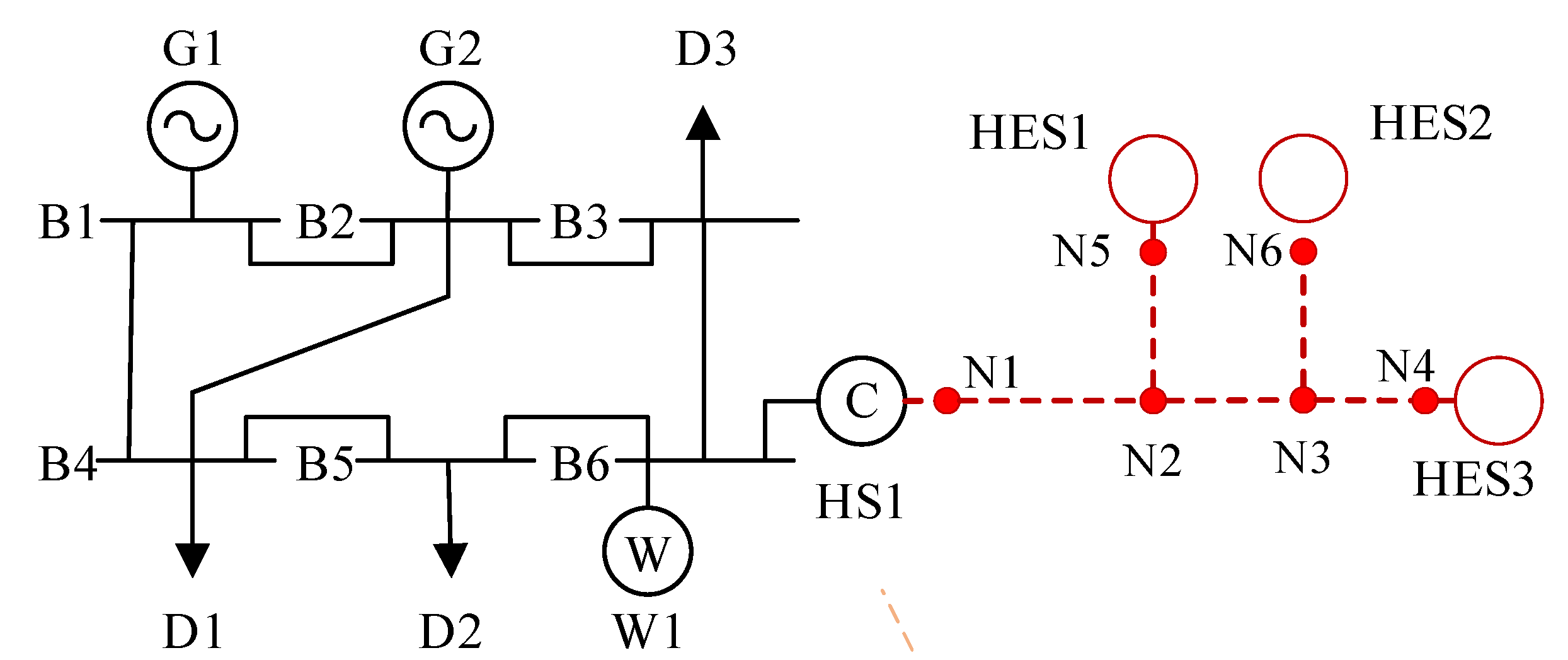
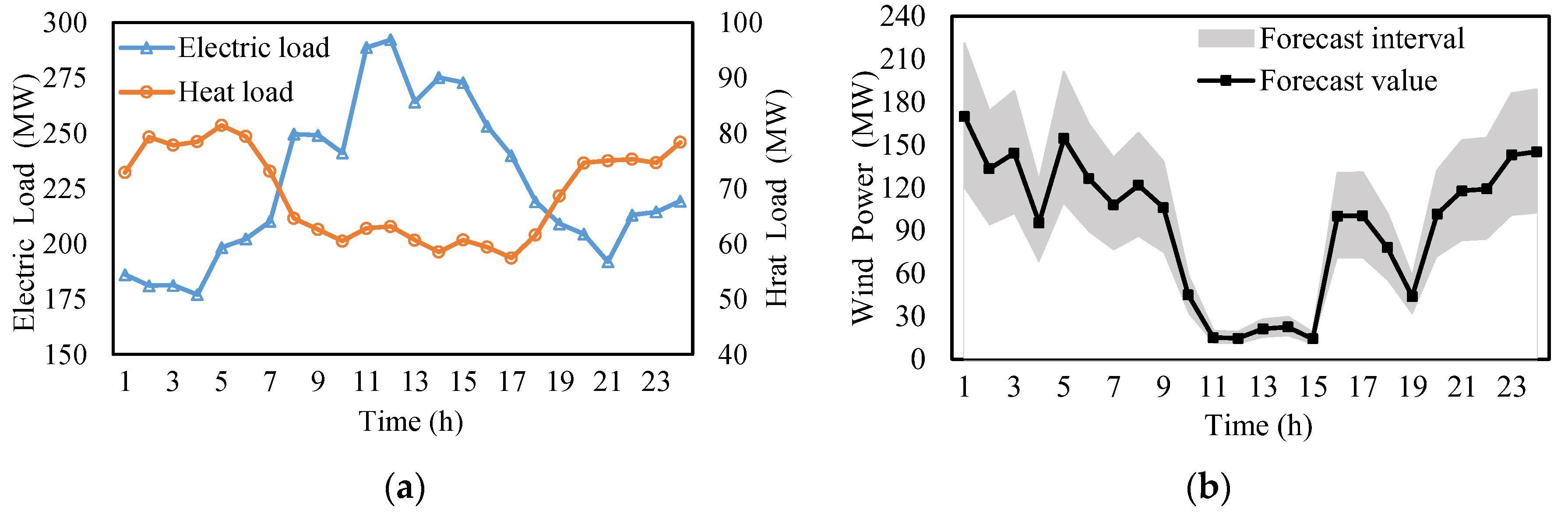
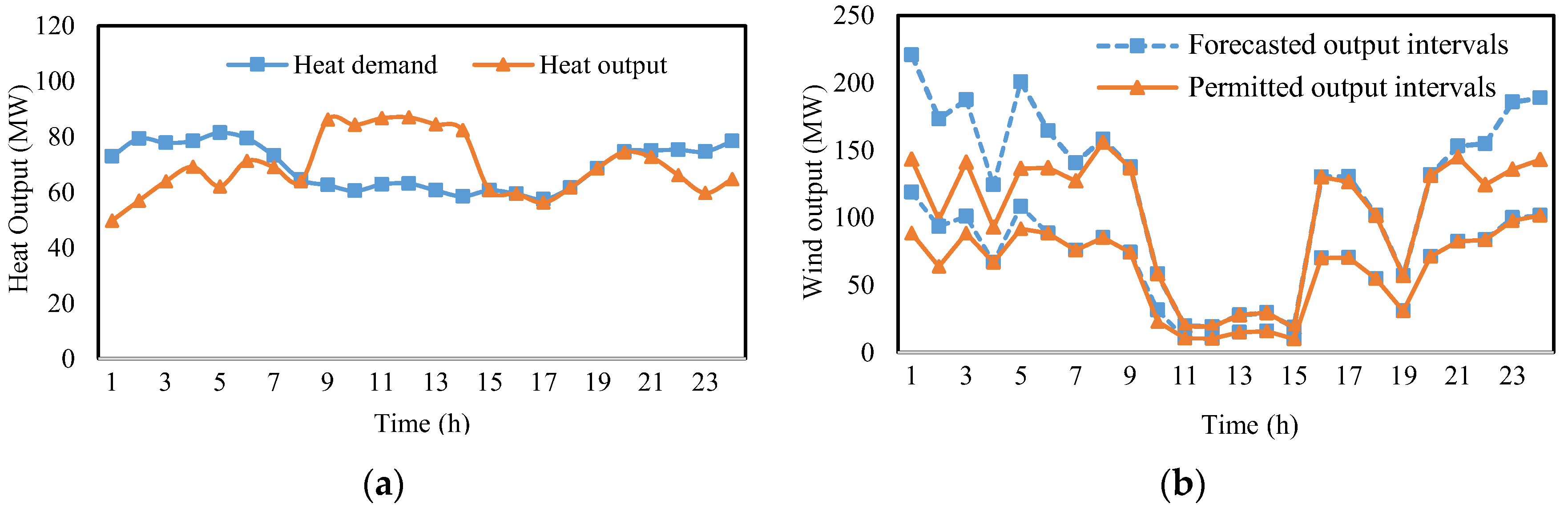
For brevity, the R-CHPD in (40) can be written in a compact form

$$\begin{array}{ccc}\underset{\mathit{x},\widetilde{\underset{¯}{\mathit{y}}},\overline{\tilde{\mathit{y}}}}{\min }& \mathit{f}\left(\mathit{x},\widetilde{\underset{¯}{\mathit{y}}},\overline{\tilde{\mathit{y}}}\right)& \\ s.t.& \mathit{D}\mathit{x}+\mathit{F}\tilde{\mathit{y}}\le \mathit{c},\forall \tilde{\mathit{y}}\in \left[\widetilde{\underset{¯}{\mathit{y}}},\overline{\tilde{\mathit{y}}}\right]& \left(a\right)\\ & \widetilde{\underset{¯}{\mathit{y}}}\le \underset{¯}{\mathit{y}},\overline{\tilde{\mathit{y}}}\le \overline{\mathit{y}}& \left(b\right)\end{array}$$

(41)

where $\mathit{x}$ refers to variables $P_{i,t}^G$, $P_{i,t}^{CHP}$, $r{u}_{i,t}$, $r{d}_{i,t}$, $\Delta r{u}_{i,t}$, $\Delta r{d}_{i,t}$, $R_t^U$, $R_t^D$, $L_{l,t}^U$, $L_{l,t}^D$, $H_{i,t}^{CHP}$, ${\lambda }_{i,t,j}$, $T_{n,t}^{NS}$, $T_{n,t}^{NR}$, $T_{j,t}^{PS,in}$, $T_{j,t}^{PS,out}$, $T_{j,t}^{PR,in}$, and $T_{j,t}^{PR,out}$. The $\widetilde{\underset{¯}{\mathit{y}}}$ and $\overline{\tilde{\mathit{y}}}$ are variable vectors that represent ${\widetilde{\underset{¯}{p}}}_{i,t}^W$ and ${\overline{\tilde{p}}}_{i,t}^W$, respectively. The $\tilde{\mathit{y}}$ is an uncertainty parameter vector that denotes the actual output of wind power ${\tilde{p}}_{i,t}^W$. $\mathit{D}\mathit{x}+\mathit{F}\tilde{\mathit{y}}\le \mathit{c}$ refers to constraints (5)–(19), (21)–(24), and (29)–(38). $\widetilde{\underset{¯}{\mathit{y}}}\le \underset{¯}{\mathit{y}},\overline{\tilde{\mathit{y}}}\le \overline{\mathit{y}}$ corresponds to constraints (30).

In (41), there is $\mathit{D}\mathit{x}+\mathit{F}\tilde{\mathit{y}}\le \mathit{c}$ for $\forall \tilde{\mathit{y}}\in \left[\widetilde{\underset{¯}{\mathit{y}}},\overline{\tilde{\mathit{y}}}\right]$, which is represented without loss generality as

$$\max \left\{\mathit{D}\mathit{x}+\mathit{F}\tilde{\mathit{y}}|\tilde{\mathit{y}}\in \left[\widetilde{\underset{¯}{\mathit{y}}},\overline{\tilde{\mathit{y}}}\right]\right\}\le c$$

(42)

i.e.,

$$\left\{\begin{array}{cc}{\mathit{D}}_{\mathit{i}}\mathit{x}+\underset{\tilde{\mathit{y}}}{\max }\left({\mathit{F}}_{\mathit{i}}\tilde{\mathit{y}}\right)\le c_i& \left(a\right)\\ \tilde{\mathit{y}}\in \left[\widetilde{\underset{¯}{\mathit{y}}},\overline{\tilde{\mathit{y}}}\right]& \left(b\right)\end{array}\right.$$

(43)

where ${\mathit{D}}_i$ and ${\mathit{F}}_i$ is row i of the matrix $\mathit{D}$ and $\mathit{F}$, respectively. ${\mathit{c}}_i$ is entry i of the vector $\mathit{c}$. Equation (43) can be further transformed into

$$\left\{\begin{array}{cc}{\mathit{D}}_{\mathit{i}}\mathit{x}+\underset{\tilde{\mathit{y}}}{\max }\left({\mathit{F}}_{\mathit{i}}\left(\widetilde{\underset{¯}{\mathit{y}}}+\mathit{w}\left(\overline{\tilde{\mathit{y}}}-\widetilde{\underset{¯}{\mathit{y}}}\right)\right)\right)\le {\mathit{c}}_{\mathit{i}},\forall i& \left(a\right)\\ 0\le \mathit{w}\le 1& \left(b\right)\end{array}\right.$$

(44)

and the dual problem is expressed as

$$\begin{array}{cc}\underset{{\mathit{u}}_{\mathit{i}}}{\min }& {\mathit{D}}_{\mathit{i}}\mathit{x}+{\mathit{F}}_{\mathit{i}}\widetilde{\underset{¯}{\mathit{y}}}+{{\displaystyle \mathbf{1}}}_{}^{\mathit{T}}{\mathit{u}}_{\mathit{i}}\\ s.t.& {\mathit{u}}_{\mathit{i}}\ge {\mathit{F}}_{\mathit{i}}\left(\overline{\tilde{\mathit{y}}}-\widetilde{\underset{¯}{\mathit{y}}}\right)\end{array},\forall i$$

(45)

Based on duality theory, Equation (46) holds.

$${\mathit{D}}_{\mathit{i}}\mathit{x}+{\mathit{F}}_{\mathit{i}}\tilde{\mathit{y}}\le {\mathit{D}}_{\mathit{i}}\mathit{x}+{\mathit{F}}_{\mathit{i}}\widetilde{\underset{¯}{\mathit{y}}}+{{\displaystyle \mathbf{1}}}_{}^{\mathit{T}}{\mathit{u}}_{\mathit{i}},\forall i$$

(46)

Consequently, (41) is equivalent to the following equivalent models:

$$\begin{array}{cc}\underset{\mathit{x},\widetilde{\underset{¯}{\mathit{y}}},\overline{\tilde{\mathit{y}}}}{\min }& \mathit{f}\left(\mathit{x},\widetilde{\underset{¯}{\mathit{y}}},\overline{\tilde{\mathit{y}}}\right)\\ s.t.& {\mathit{D}}_{\mathit{i}}\mathit{x}+{\mathit{F}}_{\mathit{i}}\widetilde{\underset{¯}{\mathit{y}}}+{{\displaystyle \mathbf{1}}}_{}^{\mathit{T}}{\mathit{u}}_{\mathit{i}}\le \mathit{c},\forall \mathit{i}\\ & {\mathit{u}}_{\mathit{i}}\ge {\mathit{F}}_{\mathit{i}}\overline{\tilde{\mathit{y}}}-{\mathit{F}}_{\mathit{i}}\widetilde{\underset{¯}{\mathit{y}}},\forall \mathit{i}\\ & \begin{array}{c}\widetilde{\underset{¯}{\mathit{y}}}\le \underset{¯}{\mathit{y}},\overline{\tilde{\mathit{y}}}\le \overline{\mathit{y}},\\ {\mathit{u}}_{\mathit{i}}\ge \mathit{0}.\end{array}\end{array}$$

(47)

The model presented in (47) is a quadratic programming problem, which can be handled directly. However, when the TPS and DHS are managed by different entities, it is impractical to solve (47) in a centralized manner. The use of the heterogeneous decomposition method allows for efficient and effective management of the TPS and DHS. By decomposing the problem and finding distributed solutions, the overall optimization of the R-CHPD system can be achieved. Due to the fact that distributed solution methods are not the focus of this paper, no further description of these is provided here. The detailed solution process can be found in [15].

4. Case Study

The performance of the proposed robust interval optimization method is tested using a 6-bus EPS connecting with a 6-node DHS (P6H6), as shown in Figure 1. Figure 2a shows the electric loads and heat loads, and Figure 2b shows the forecast wind power. The transmission interface capacity is 50 MW. For conciseness, other system parameters are provided in [16]. To analyze the performance of the proposed model, three cases were established:

Case 1: isolated heat and power dispatch (IHPD) mode, where the EPS and DHS are independently operated. In this mode, the DHS operator dispatches the CHP units to meet the heat demand. Subsequently, the EPS determines the unit dispatch strategies based on the constraints of CHP heat output.

Case 2: coordinated heat and power dispatch (CHPD) mode, where the EPS and DHS are dispatched in a coordinated manner. In this case, the CHP units are optimally dispatched to satisfy both the heat and power demands.

Case 3: Based on Case 2, the wind power output uncertainty is considered, and R-CHPD is performed.

The major results of the study are presented in

Table 1. Test results.

Title 1	IHPD	CHPD	R-CHPD
${\displaystyle \sum _{t\in {\rm T}}}{C}_t^G$	USD 79,603	USD 76,548	USD 77,362
${\displaystyle \sum _{t\in {\rm T}}}{C}_t^{CHP}$	USD 28,329	USD 26,421	USD 26,958
${\displaystyle \sum _{t\in {\rm T}}}{C}_t^W$	USD 1506	USD 501	USD 1703
Total cost	USD 109,438	USD 103,470	USD 106,023

and Figure 3. In the case of IHPD, the heat output of CHP units is always matched to the heat demand. Due to the heat-driven nature of CHP units, the power output of these units needs to be maintained at a high level during the night, leading to significant curtailment of wind power. As shown in Table 1, the cost of wind power curtailment amounts to USD 1506.

In CHPD, the heat output of the CHP unit is not strictly limited by heat loads. It utilizes the heat storage of the DHN so that the output of CHP units can be flexibly adjusted for better wind power penetration. In contrast to IHPD, the wind curtailment decreases by 3.84%, and the total cost is reduced by 5.45%.

It should be noted that in the CHPD, the wind power output is assumed to be certain, which may not be realistic in practice. In order to account for wind power uncertainties, R-CHPD requires non-CHP units to maintain a larger reserve capacity to ensure system operational security. As a result, the total cost increases by 2.47% compared to CHPD. However, it is important to highlight that the dispatch strategies in R-CHPD remain feasible as long as the wind power generation falls within the permitted output interval.

5. Conclusions

To address the issue of wind curtailment, this paper proposes a robust interval optimization technique for CHPD. Instead of using fixed numerical values as control targets for wind farms, interval values are utilized, which allows for a more flexible and adaptable approach. It is important to note that while this paper focuses on the uncertainty of wind power output, the robust interval optimization method can also be applied to other uncertainties present in the system. For instance, in real-world scenarios, there may be uncertainty in both the electric and heat loads. In such cases, these uncertain loads can be treated as negative outputs and combined with the wind power output to construct the uncertainty set.

One limitation of this method is that when the prediction error is large, the obtained results may be too conservative. In other words, the system may overly prioritize robustness at the expense of economic efficiency. To address this issue, the next step in our research is to improve the prediction interval. By refining the prediction interval, we aim to strike a balance between robustness and economy, ensuring that the system operates optimally while accounting for uncertainties. By enhancing the prediction interval, we expect to achieve a more accurate estimation of the uncertainty bounds, allowing for better decision-making in resource planning and emergency measures. This will ultimately lead to improved system performance and the effective utilization of the robust interval optimization technique in CHPD.

References

1. Li, Z.; Wu, W.; Shahidehpour, M.; Wang, J.; Zhang, B. Combined Heat and Power Dispatch Considering Pipeline Energy Storage of District Heating Network. IEEE Trans. Sustain. Energy 2016, 7, 12–22. [Google Scholar] [CrossRef]
2. Chen, X.; McElroy, M.B.; Kang, C. Integrated Energy Systems for Higher Wind Penetration in China: Formulation, Implementation and Impacts. IEEE Trans. Power Syst. 2017, 33, 1309–1319. [Google Scholar] [CrossRef]
3. Dai, Y.; Chen, L.; Min, Y.; Mancarella, P.; Chen, Q.; Hao, J.; Hu, K.; Xu, F. Integrated Dispatch Model for Combined Heat and Power Plant With Phase-Change Thermal Energy Storage Considering Heat Transfer Process. IEEE Trans. Sustain. Energy 2018, 9, 1234–1243. [Google Scholar] [CrossRef]
4. Dai, Y.; Chen, L.; Min, Y.; Mancarella, P.; Chen, Q.; Hao, J.; Hu, K.; Xu, F. A General Model for Thermal Energy Storage in Combined Heat and Power Dispatch Considering Heat Transfer Constraints. IEEE Trans. Sustain. Energy 2018, 9, 1518–1528. [Google Scholar] [CrossRef]
5. Wu, C.; Gu, W.; Jiang, P.; Li, Z.; Cai, H.; Li, B. Combined Economic Dispatch Considering the Time-Delay of District Heating Network and Multi-Regional Indoor Temperature Control. IEEE Trans. Sustain. Energy 2018, 9, 118–127. [Google Scholar] [CrossRef]
6. Zheng, J.; Zhou, Z.; Zhao, J.; Wang, J. Effects of the Operation Regulation Modes of District Heating System on an Integrated Heat and Power Dispatch System for Wind Power Integration. Appl. Energy 2018, 230, 1126–1139. [Google Scholar] [CrossRef]
7. Huang, X.; Xu, Z.; Sun, Y.; Xue, Y.; Wang, Z.; Liu, Z.; Li, Z.; Ni, W. Heat and Power Load Dispatching Considering Energy Storage of District Heating System and Electric Boilers. J. Mod. Power Syst. Clean Energy 2018, 6, 992–1003. [Google Scholar] [CrossRef]
8. Wang, K.; Xue, Y.; Guo, Q.; Shahidehpour, M.; Zhou, Q.; Wang, B.; Sun, H. A Coordinated Reconfiguration Strategy for Multi-Stage Resilience Enhancement in Integrated Power Distribution and Heating Networks. IEEE Trans. Smart Grid 2023, 14, 2709–2722. [Google Scholar] [CrossRef]
9. Du, Y.; Xue, Y.; Lu, L.; Yu, C.; Zhang, J. A Bi-Level Co-Expansion Planning of Integrated Electric and Heating System Considering Demand Response. Front. Energy Res. 2022, 10, 999948. [Google Scholar] [CrossRef]
10. Li, Y.; Zou, Y.; Tan, Y.; Cao, Y.; Liu, X.; Shahidehpour, M.; Tian, S.; Bu, F. Optimal Stochastic Operation of Integrated Low-Carbon Electric Power, Natural Gas, and Heat Delivery System. IEEE Trans. Sustain. Energy 2018, 9, 273–283. [Google Scholar] [CrossRef]
11. Majidi, M.; Mohammadi-Ivatloo, B.; Anvari-Moghaddam, A. Optimal Robust Operation of Combined Heat and Power Systems with Demand Response Programs. Appl. Therm. Eng. 2019, 149, 1359–1369. [Google Scholar] [CrossRef]
12. Nazari-Heris, M.; Mohammadi-Ivatloo, B.; Gharehpetian, G.B.; Shahidehpour, M. Robust Short-Term Scheduling of Integrated Heat and Power Microgrids. IEEE Syst. J. 2019, 13, 3295–3303. [Google Scholar] [CrossRef]
13. Shui, Y.; Gao, H.; Wang, L.; Wei, Z.; Liu, J. A Data-Driven Distributionally Robust Coordinated Dispatch Model for Integrated Power and Heating Systems Considering Wind Power Uncertainties. Int. J. Electr. Power Energy Syst. 2019, 104, 255–258. [Google Scholar] [CrossRef]
14. Du, Y.; Xue, Y.; Wu, W.; Shahidehpour, M.; Shen, X.; Wang, B.; Sun, H. Coordinated Planning of Integrated Electric and Heating System Considering the Optimal Reconfiguration of District Heating Network. IEEE Trans. Power Syst. 2023. early access. [Google Scholar] [CrossRef]
15. Xue, Y.; Li, Z.; Lin, C.; Guo, Q.; Sun, H. Coordinated Dispatch of Integrated Electric and District Heating Systems Using Heterogeneous Decomposition. IEEE Trans. Sustain. Energy 2020, 11, 1495–1507. [Google Scholar] [CrossRef]
16. Test Data for R-CHPD. Available online: https://docs.google.com/spreadsheets/d/1TNrEsWwrCDvDcEuHb7VnUQcul6cFcCoN/edit?usp=sharing&ouid=115924522171410221124&rtpof=true&sd=true (accessed on 26 July 2023).
Figure 1. P6H6 system.
Electronics 12 03706 g001
Figure 2. (a) Electric load and heat load; (b) forecast wind power.
Electronics 12 03706 g002
Figure 3. (a) Heat output in Case 2; (b) wind output of W1 in Case 3.
Electronics 12 03706 g003