Multi-Scale Spatial–Spectral Attention-Based Neural Architecture Search for Hyperspectral Image Classification

Abstract

Convolutional neural networks (CNNs) are indeed commonly employed for hyperspectral image classification. However, the architecture of cellular neural networks typically requires manual design and fine-tuning, which can be quite laborious. Fortunately, there have been recent advancements in the field of Neural Architecture Search (NAS) that enable the automatic design of networks. These NAS techniques have significantly improved the accuracy of HSI classification, pushing it to new levels. This article proposes a Multi-Scale Spatial–Spectral Attention-based NAS, MS³ANAS) framework for HSI classification to automatically design a neural network structure for HSI classifiers. First, this paper constructs a multi-scale attention mechanism extended search space, which considers multi-scale filters to reduce parameters while maintaining large-scale receptive field and enhanced multi-scale spectral–spatial feature extraction to increase network sensitivity towards hyperspectral information. Then, we combined the slow–fast learning architecture update paradigm to optimize and iteratively update the architecture vector and effectively improve the model’s generalization ability. Finally, we introduced the Lion optimizer to track only momentum and use symbol operations to calculate updates, thereby reducing memory overhead and effectively reducing training time. The proposed NAS method demonstrates impressive classification performance and effectively improves accuracy across three HSI datasets (University of Pavia, Xuzhou, and WHU-Hi-Hanchuan).

1. Introduction

Hyperspectral remote sensing images (HSIs) capture abundant spatial–spectral information across numerous spectral bands, enabling effective differentiation of surface cover. Therefore, hyperspectral images are widely used in environmental science [1], mineral exploration [2], plant detection [3], military reconnaissance [4], and so on.

HSIs can extract feature vectors containing thousands of bands from each spatial pixel position. In practice, there are two phenomena in HSIs: (1) Different objects have similar spectral characteristics; (2) The same object at different positions has different spectral characteristics [5]. This is due to the influence of the imaging factors of atmosphere and light, which leads to the obvious spectral shift between different scenes.

HSI classification is based on pixel level. In the past decade, various traditional machine learning methods, including the K-nearest neighbor (KNN) algorithm, Support Vector Machine (SVM) [6], and others, have been widely employed for pixel-level HSI classification [7].

Compared with traditional classification algorithms, deep learning-based HSI classification methods have demonstrated their effectiveness in extracting robust features from HSIs, and they have better classification performance. HSI classification methods utilizing CNN can be classified into three categories based on the feature extraction approach employed: spectral CNN [8,9,10], spatial CNN [11,12], and spectral–spatial CNN [13,14,15,16,17]. However, many excellent deep classification network architectures need to be designed manually, such as ResNet [16], DenseNet [18], VGG [19], and GoogLeNet [20].

Designing an efficient network architecture for HSI classification is a challenging task that involves significant time, energy, and a large number of verification experiments, making it difficult to achieve manually. In addition, HSI data has obvious differences in the number of frequency bands, spectral range, and spatial resolution, so the network architectures applied to different HSI data classifications are also different [21]. It is necessary to design different network architectures for HSI classification, which requires a large amount of work to adjust parameters, resulting in a large consumption of time and resource costs. Therefore, a natural idea is to automate the neural network design process and minimize human assistance.

The need to enhance the efficiency of automatic neural network design technology is motivated by both the expense of computing resources and the burden of parameter adjustment [22]. NAS has been applied to many tasks and has achieved remarkable results, such as speech recognition [23], computer vision [24], and so on. The objective of Neural Architecture Search (NAS) is to automate the construction of high-performance neural network structures by selecting and combining various neural operations from predefined search spaces. Previous approaches to NAS have employed various methods, including reinforcement learning algorithm (RL) [25], evolutionary algorithm (EA) [26], and gradient-based methods, to perform architecture searches. The reinforcement learning algorithm regards NAS search as an agent behavior, and network construction is realized through different behaviors and rewards, which can evaluate the performance of the acquired network structure. Representation and optimization of agent strategy are two key contents of network structure search using reinforcement learning [25]. The evolutionary algorithm uses a genetic algorithm to realize selection, crossover, and compilation to initialize the search of individuals and cyberspace [27,28].

Among various NAS methods, DARTS and population-based NAS are among the most popular ones because they have unique advantages in dealing with many challenging tasks. DARTS mainly benefits from the advantage of relaxing the search space into a continuous and high search efficiency. The population-based NAS mainly benefits from the advantages of diverse candidate structures within the population and involves genetic operators to drive the search process. As the term itself indicates, the population-based NAS represents a candidate architecture for each individual. Collaboration between candidate architectures can eliminate poor and well-preserved competition and push the overall optimization. At present, most population-based NAS methods use genetic algorithms or genetic programming [25,29] to simulate natural evolution processes, which requires careful design of random crossover mutation operators. For example, the population-based NAS method [30] has designed 11 mutation operators to modify the attributes of the network, including changing the learning rate, resetting weights, inserting convolutions, etc. This study shows that designing different genetic operators has good feasibility, and neural networks can be developed and changed from an architectural perspective. Although the population-based NAS has good performance, many current methods mainly have the drawback of low computational efficiency.

Whether based on reinforcement learning or population algorithm, NAS realizes automation through resource-consuming search. To minimize resource usage, one-shot NAS techniques using hypernetworks have been devised [31,32]. DARTS, a one-shot NAS approach employing a discernible search strategy [32], incorporates weight sharing to integrate hypernetwork training and the search for the optimal candidate architecture. This integration effectively curtails computing resource wastage. At the same time, the gradient-based method is used to optimize the over-parameterized hypernetwork. However, the greater number of weight parameters in DARTS compared to architecture parameters imposes constraints on architecture optimization, leading to performance crashes [31]. Essentially, this is because DARTS’ candidate results lack diversity in gradient optimization.

However, these NAS methods have their own characteristics that DARTS jointly trains the hypernetwork and only searches for the optimal solution through the gradient, so they have defects in flexibility and stability [33]. Many population-based NASs mainly rely on random crossover/mutation search, which usually requires a lot of computational cost to evaluate the performance. Therefore, this work adopts the slow–fast learning paradigm architecture update process in DARTS, which integrates the idea of population-based NAS. In addition, it can benefit from the advantages of differentiated NAS while overcoming the shortcomings of the population-based NAS [34].

NAS technology can efficiently automate this process, not only to find the weight of specific image classification tasks but also to obtain the best network architecture. The incorporation of NAS offers an excellent solution for HSI data classification, relieving individuals from the burdensome task of network architecture design. Chen et al. pioneered the integration of the DARTS method into the HSI classification task, presenting their proposed approach as 3D-Auto-CNN with Cutout (CNAS) [35] and leveraging point-by-point convolution to reduce the spectral dimensions of HSI to several dozens. Subsequently, DARTS is utilized to search for a neural network architecture that is well-suited for the HSI dataset. This approach aims to minimize redundancy and repetition.

In recent years, the rise of attention mechanisms has brought new research directions to deep learning. Many researchers use different scales of attention mechanisms to extract the effective features of different objects in HSI data and classify them effectively. To reduce repetition, there have been several approaches proposed in the literature for HSI classification. Wang introduced the Squeeze and Excitation (SE) [36] module, which adaptively learns the weights of different spectral bands and adjacent pixels in HSI. This module helps capture relevant information for classification. Roy et al. [37] introduced a novel method named A2S2K-ResNet (Attention-based Adaptive Spectral Spatial Kernel Improved Residual Network). This approach integrates spectral attention to effectively capture discriminative features for HSI classification. These methods contribute to reducing redundancy and improving the efficiency of HSI classification tasks. However, in the field of HSI classification for NAS applications, there is limited search space utilizing multi-scale attention mechanisms. In addition, various samples in the HSI dataset exhibit long- tailed distributions, resulting in imbalanced HSI classification results. In light of the aforementioned approaches, we propose a novel method that utilizes a multi-scale search space combined with multi-scale spatial–spectral attention. This approach aims to enhance the extraction of significant spectral–spatial information while suppressing redundant information and noise. By incorporating this multi-scale attention mechanism, our method effectively improves the accuracy of classification while reducing computational complexity. Furthermore, it helps to minimize repetition and redundancy in the HSI classification process.

Building upon the aforementioned discussion, we present a novel NAS method that encompasses the automatic design of a search space for multi-scale attention mechanisms and a search strategy based on the slow–fast paradigm. The key contributions of this research can be summarized as follows:

• To address the issue of redundancy, we have proposed a highly effective NAS classification framework called Multi-Scale Spatial–Spectral Attention-based NAS (MS³ANAS). By carefully analyzing the characteristics of HSI, we have designed a multi-scale search space that incorporates rich spatial–spectral attention mechanisms. This search space consists of seven convolutional operators, each equipped with attention mechanisms of different scales. The search process can automatically learn to add attention modules to appropriate locations in the architecture to fully explore the spectral and spatial information of HSIs for classification.
• The slow–fast learning paradigm was quoted for NAS, which further optimizes the overall architecture vector through pseudo gradient iteration, stabilizing the optimal search process, which improves the update and rate of convergence speed of the architecture for HSI classification.
• To better train the HSI classification model, the Lion optimizer has been introduced, which not only effectively improves the accuracy of HSI data classification but also reduces memory overhead and training time because the algorithm only tracks momentum and uses symbol operations to calculate updates.

2. Materials and Methods

2.1. Search Framework

Figure 1 illustrates the proposed NAS framework for HSI classification in this paper. Initially, the hyperspectral image is divided into patches using a sliding window approach. These patches are then fed into the automatic architecture search model, which consists of both normal cells and reduction cells. Secondly, the NAS network includes supernet architecture search and final network optimization. We designed a multi-scale attention mechanism search operator for the search space (The different colored arrows represent different candidate operations), enhancing the ability to extract multi-scale spectral–spatial features from HSI data, thereby improving classification performance. Then, we utilized the slow–fast learning paradigm to effectively update the overall architecture vector, improving the efficiency of constructing hypergrid architecture units. Finally, we introduced the Lion optimizer to accelerate model convergence and alleviate model memory overhead.

2.2. Neural Architecture Search Algorithm

MS³ANAS consists of three architecture search components: the search space of the multi-scale expanding attention mechanism, the search strategy of the slow–fast learning paradigm, and the Lion optimizer. Here is a detailed explanation of each component.

2.2.1. Multi-Scale Attention Mechanism Expanded Search Space

• Multiple attention mechanism guided search space

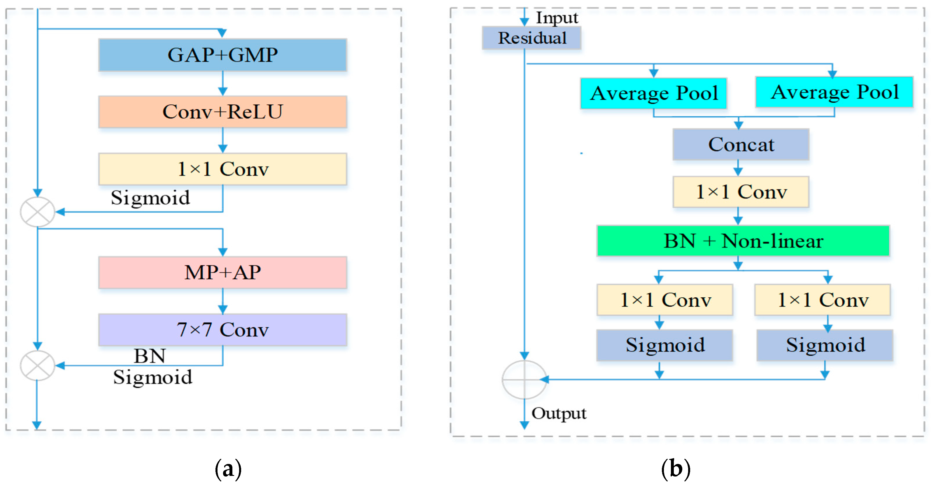
Applying different attention mechanisms to different datasets may face varying challenges. For example, in some HIS datasets, it may be more challenging to use spatial attention mechanisms due to strong correlations between data. In contrast, it may be more difficult to use channel attention mechanisms due to highly variable features. Moreover, the performance of attention mechanisms can also be affected by factors such as dataset size and quality, model architecture, and hyperparameters. Therefore, it is important to choose appropriate attention mechanisms based on different HSI datasets and tasks to achieve optimal performance and effectiveness. In addition, various samples in the HSI dataset exhibit long-tailed distributions, resulting in imbalanced HSI classification results. We propose a multiple search space with rich attention for HSI classification, which can effectively improve classification accuracy and reduce computational complexity. We select four types of attention mechanisms to form it. They are the convolutional block attention module (CBAM) [38], squeeze-and-excitation (SE) module [36], triplet attention (TA) module [39], and coordinate attention mechanism (CA) [40], as shown in Figure 2.

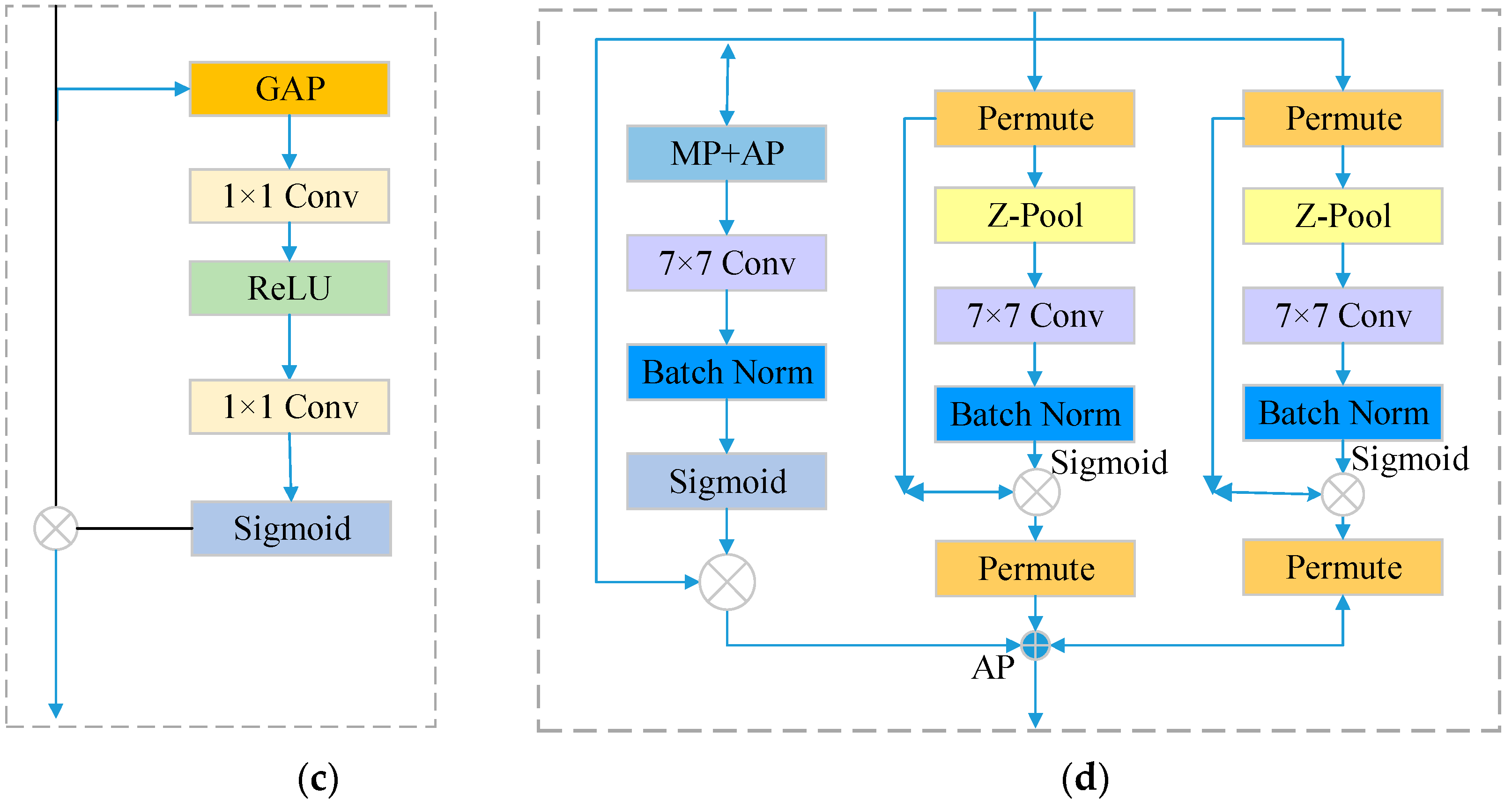
To reduce repetition, various attention mechanisms have been proposed in the literature. One such mechanism is the CBAM module, which combines channel attention and spatial attention. It aggregates spatial features by performing max-pooling on top of global average pooling. This allows the network to focus on important spatial information. Another attention mechanism is the SE module, which enhances the network’s sensitivity to informative features. It recalibrates filter responses through squeeze-and-excitation operations, improving the learning ability of convolutional layers. The TA module is composed of three parallel branches, each serving a distinct purpose. The first branch focuses on establishing spatial attention, while the other two branches aim to capture cross-dimensional interactions between the channel and spatial dimensions. The final output is obtained by averaging the outputs from these three branches. The CA mechanism learns weights by combining features at each position with their corresponding coordinate information. This mechanism effectively captures spatial correlations, leading to improved model performance. By incorporating these attention mechanisms, models can effectively reduce redundancy and improve the performance of HSI classification tasks.

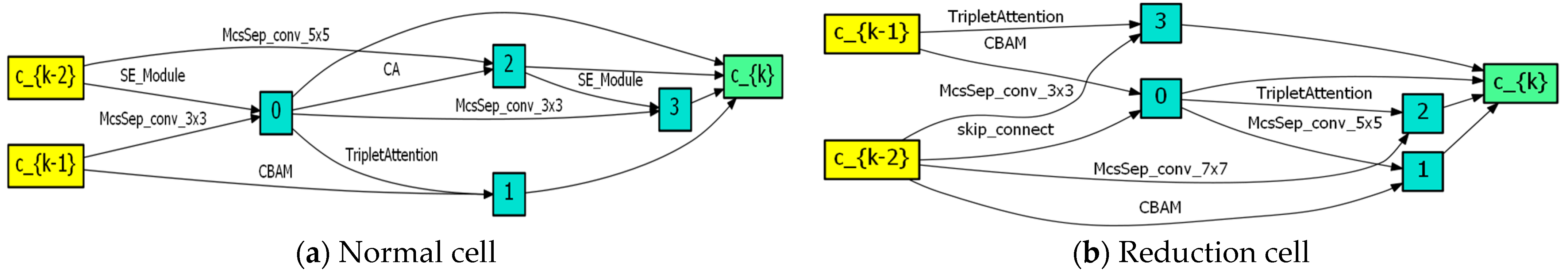
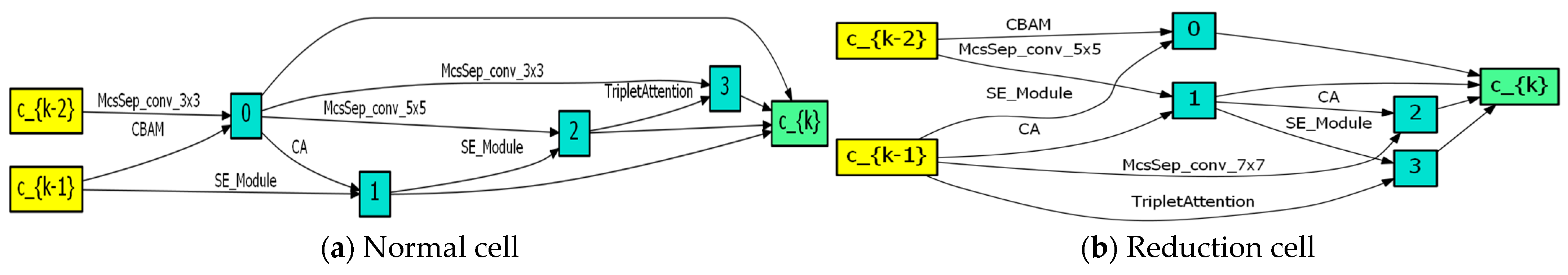
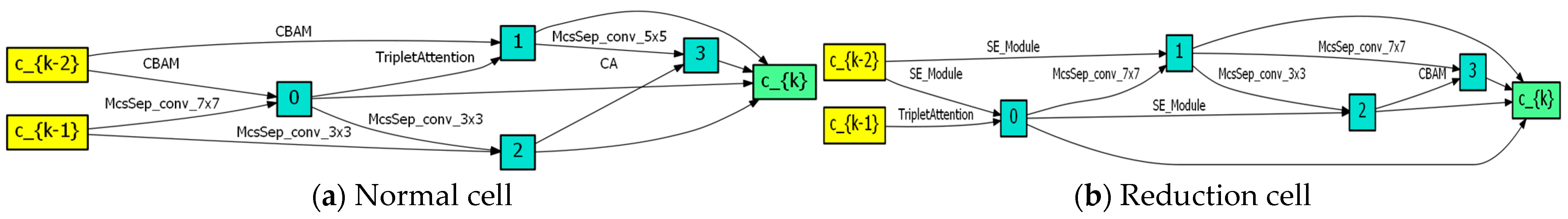
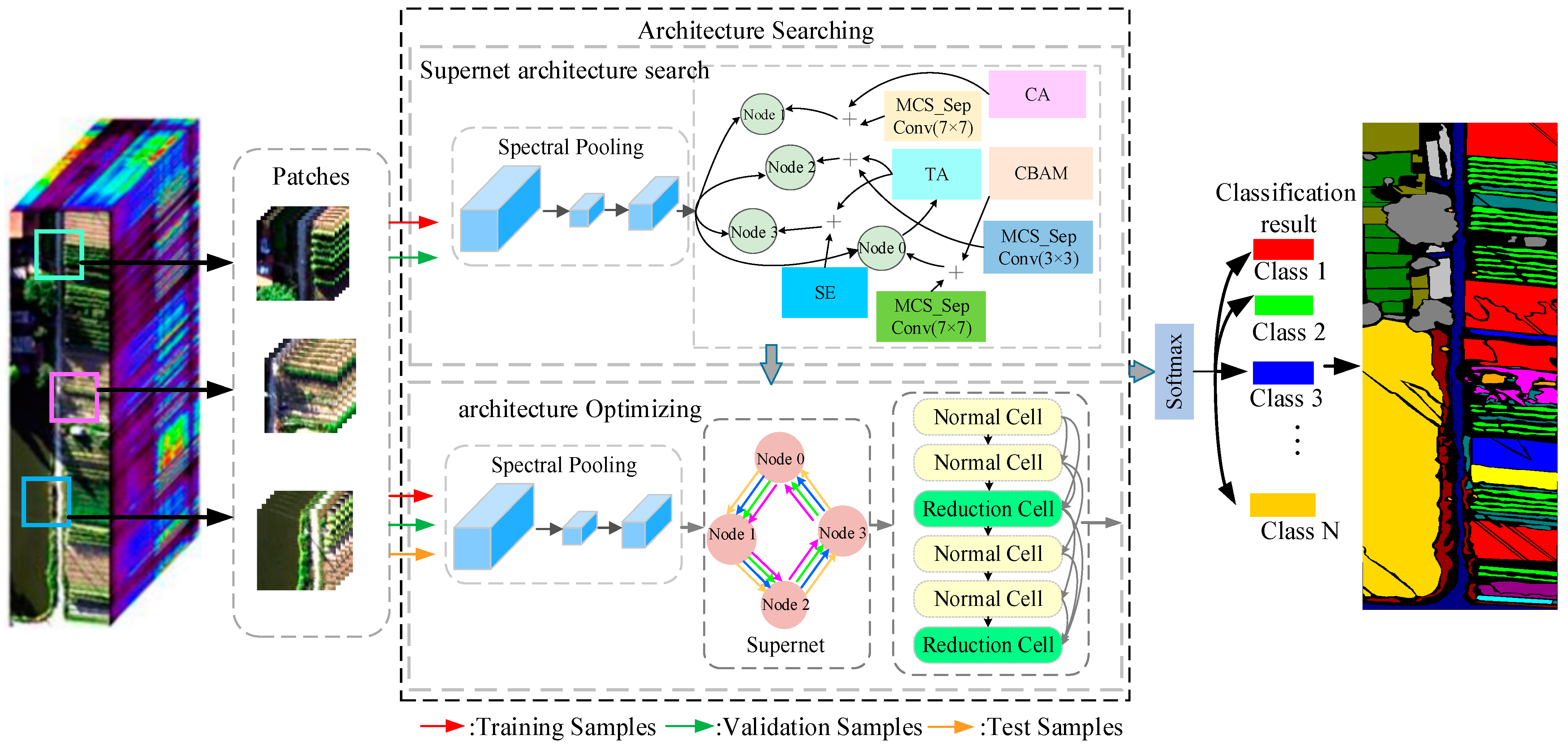
As NAS-based HSI classification requires the determination of the search space, we propose search space $O$. Formally, let $O$ denote a sequence of candidate operations (multiple attention guided operations), where each operation represents a function $p(·)$ to be applied to $s_i$. For each cell $q$, we configure an architecture parameter ${\alpha }_{p_i}^q$ for operation $p_i$. To ensure continuity of the search space, we relax the search space to allow it to be optimized via gradient descent. Specifically, we relax the architecture parameter ${\alpha }_{p_i}^q$ to be continuous, and then compute the operational probabilities for different operations by applying softmax over all ${\alpha }_{p_i}^q$.

$$R_{p_i}^q=\frac{\exp ({\alpha }_{p_i}^q)}{{\displaystyle \sum _{j=1}^n\exp ({\alpha }_{p_j}^q)}}$$

(1)

Here, $n$ represents the number of candidate operations available. The larger value of $R_{p_i}^q$ indicates a higher likelihood of selecting the representative operation. The output of the cell is obtained by taking the weighted sum of all possible operations.

$$\overline{p}(y_i)={\displaystyle \sum _{p\in P}{R}_{p_i}^q}{p}_i(y_i)$$

(2)

The notation $p_i(y_i)$ signifies the application of operation $p_i$ on input $y_i$. Consequently, the search process is transformed into a learning process of a set of architectural parameters {${\alpha }_{p_i}^q$}. Furthermore, as the network weights $w$ also need to be learned, we are required to solve the following bi-level optimization problem.

$$\underset{\alpha }{\min }{ℒ}_{val}(w*,\alpha )$$

(3)

$$s.t.\mathrm{w}*=\mathrm{argmin}{ℒ}_{train}(w,\alpha )$$

(4)

The purpose of the above formulae is to search for the architectural parameters that minimize the validation loss ${ℒ}_{val}(w*,\alpha )$, and the network weights $w*$ are obtained by minimizing the training loss ${ℒ}_{train}(w,\alpha )$. It is important to note that the training loss and the validation loss are identical.

The objective of the aforementioned formulae is to search for architectural parameters that minimize the validation loss ${ℒ}_{val}(w*,\alpha )$, while the network weights $w*$ are obtained by minimizing the training loss ${ℒ}_{train}(w,\alpha )$. It is crucial to emphasize that the training loss and the validation loss are indeed the same.

2.

Multi-scale attention mechanism search space

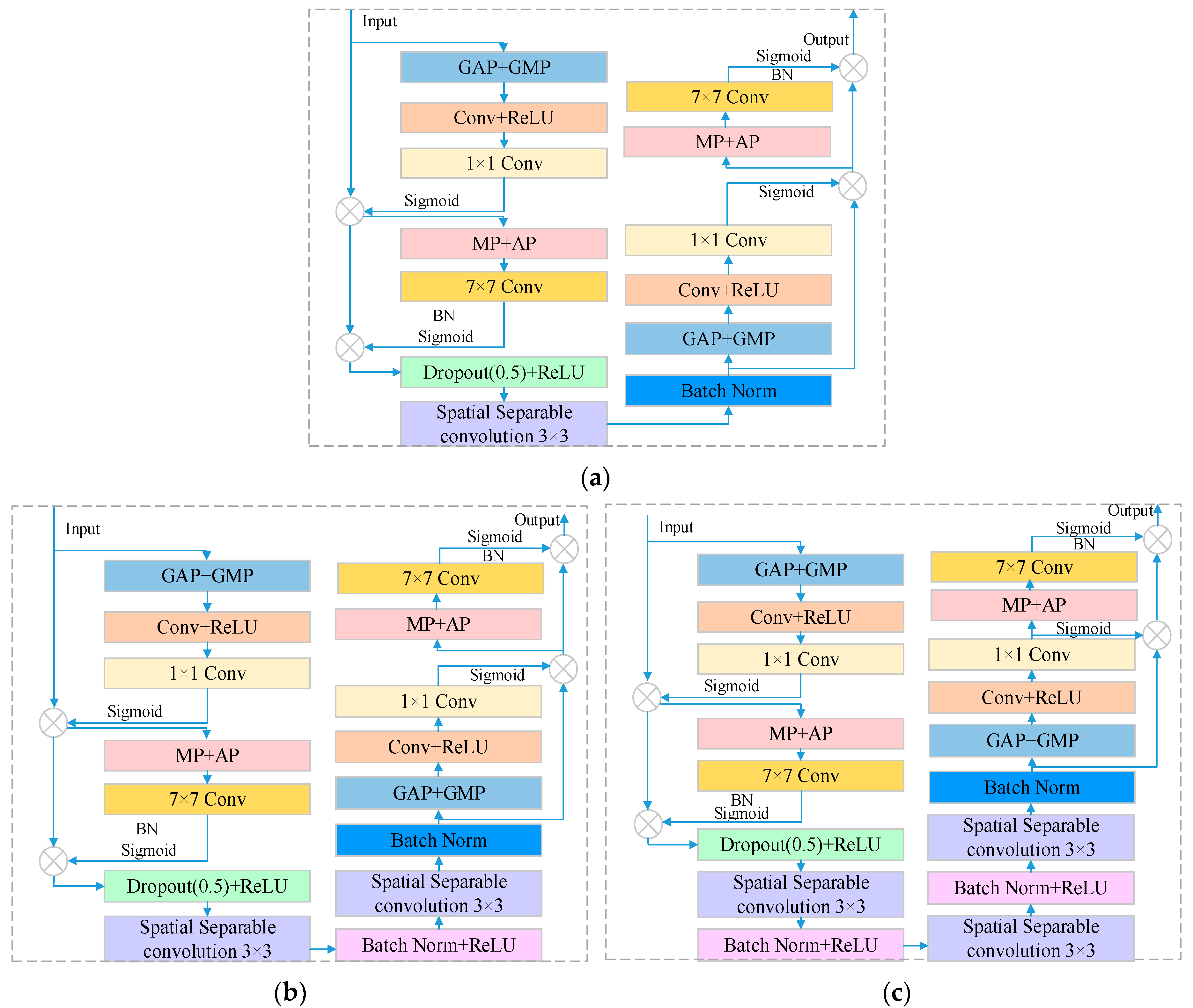
Different types of convolutions have varying computational requirements and parameter counts. Building deeper models can be challenging due to the expensive parameters and time required for high-dimensional convolutions. This can limit the efficiency and feasibility of constructing deeper models. Therefore, high-dimensional convolutions are often replaced with lower-dimensional separable convolutions to alleviate this issue. The novel operation MCS_sepConv_(b × b) (b = 3, 5, 7) in the search space combines spectral–spatial CBAM with spatial separable convolution [41], which helps to extract deeper spectral–spatial features, and it can enhance the spectral–spatial adaptive learning ability of the I data. In addition, we use small filters to reduce parameters while maintaining a large-scale receptive field. We have strengthened the ability to extract scale spectral–spatial features from data, thereby improving classification performance. MCS_sepConv(b = 3, 5, 7) with different scales are as shown in Figure 3.

MCS_sepConv_(b × b) refers to a set of convolutional operators that are commonly used in remote sensing and other image-processing tasks to extract deeper spectral–spatial features. These operators consist of two separate convolutional layers, one for processing the spectral dimension and the other for processing the spatial dimension, and they are applied in a cascaded manner. By using MCS_sepConv_(b × b), the model can capture more complex and abstract features by combining spectral and spatial information.

Convolution is a widely used operation in NAS-based methodIor HSI classification. Previous research has primarily concentrated on traditional convolution techniques, depthwise separable convolution, and dilated convolution in order to reduce redundancy. However, the high-dimensional convolutional operations can lead to a large number of parameters and time consumption, making it very difficult to construct an optimal architecture. For example, depthwise separable convolution can be represented as Sep-Conv(b × b) = Conv(1 × 1)(Conv(b × b)(x)), and the parameter and Flops(floating point operations per second) calculations are:

$$P_1=C_{in}\times b\times b+1\times C_{in}\times C_{out}$$

(5)

$$\begin{array}{c}{F}_1=C_{in}\times b\times b\times H\times W+1\times 1\\ \times C_{in}\times C_{out}\times H\times W\end{array}$$

(6)

where $C_{in}\times H\times W$ is the size of the input x, and $C_{out}\times H\times W$ corresponds to the output features, where $C_{in}$ and $C_{out}$ represent the input and output spectral bands, respectively. Additionally, P₁ and F₁ represent the number of parameters and Flops. Incorporating a pointwise convolution following a depthwise convolution in the CNN can effectively extract both spatial and spectral features in a sequential manner. Assuming $C_{in}=C_{out}=C$, the number of parameters and Flops for separable convolutions is only $(1/b^2+1/C)$ of regular convolutions. If we extend the concept of separable convolution to the spatial dimensions, we can define spatial separable convolution as Spatial_SepConv(b × b) = Conv(1 × 1Conv(1 × b)(Conv(b × 1)(x)). The number of parameters and Flops for a spatial separable convolution is only $(2b+C)/(C+b^2)$ of separable convolution:

$$P_4=2\times (C_{in}\times b\times 1)+1\times 1\times C_{in}\times C_{out}$$

(7)

$$\begin{array}{l}{F}_4=2\times (C_{in}\times b\times 1\times H\times W)\\ +1\times 1\times C_{in}\times {\mathrm{C}}_{out}\times H\times W\end{array}$$

(8)

To reduce redundancy in a convolutional neural network (CNN), one approach is to use small filters instead of large-scale filters. This helps to decrease the number of parameters while still maintaining a large receptive field. This is because, in the CNN, the number of parameters and computations is directly related to the size of the input data and the convolution kernel. By using smaller filters, the number of parameters and computations can be significantly reduced. By using small filters, we can reduce the number of parameters while maintaining a large receptive field, which is important for capturing multi-scale features in HSI classification. This can be achieved by using a combination of small filters with different kernel sizes, which allows us to capture multi-scale features while reducing the number of parameters and computations.

To enhance the adaptive feature extraction capability of the designed convolution operation, a lightweight attention module called CBAM (Multi-scale Channel–Spatial Attention, MCS) is incorporated to enhance the spectral and spatial adaptive learning ability of the data cube. MCS is a combination of the Multi-scale Channel Attention (MS) mechanism and the Multi-scale Spatial Attention (MS) mechanism as follows:

$$\begin{array}{cc}\hfill Mc(F)& =\sigma (MLP(AvgPool(F)+MLP(MaxPool(F))\hfill \\ & {=(\mathrm{W}}_1{(\mathrm{W}}_0{(\mathrm{F}}_{avg}^C{\left)\right)+\mathrm{W}}_1({\mathrm{W}}_0{(\mathrm{F}}_{max}^C)))\hfill \\ \hfill F^{\prime }& =M_c(F)\otimes F\hfill \end{array}$$

(9)

$$\begin{array}{cc}\hfill Ms(F)& =\sigma (f^{7\times 7}([AvgPool(F^{\prime });MaxPool(F^{\prime })]))\hfill \\ & =(f^{7\times 7}[F{\prime }_{avg}^S;F{\prime }_{max}^S])\hfill \\ \hfill F^{″}& =M_s(F’)\otimes F’\hfill \end{array}$$

(10)

where $M_{cs}(F)=M_s(M_c(F))$ represents the spectral–spatial CBAM, which involves element-wise multiplication $\otimes$, ${\mathrm{W}}_0\in {ℝ}^{C_{in}/\mathrm{r}\times C_{in}}$,${\mathrm{W}}_1\in {ℝ}^{C_{in}\times C_{in}/r}$, sigmoid activation $\sigma$, and the 7 × 7 convolutional $f^{7\times 7}$.

As shown in

Table 1. Comparison of convolution parameters and Flops at different scales.

Operation	Convolution	Repeat	Parameters	Flops
Conv(3 × 3)	Conv(3 × 3)	-	9 × C2	9 × C2 × H × W
Conv(5 × 5)	Conv(3 × 3)	2	18 × C2	18 × C2 × H × W
Conv(7 × 7)	Conv(3 × 3)	3	27 × C2	27 × C2 × H × W
Spatial_sepconv(3 × 3)	Conv(1 × 3)(Conv(3 × 1))	-	6 × C2	6 × C × H × W
Spatial_sepconv(5 × 5)	Conv(1 × 3)(Conv(3 × 1))	2	12 × C2	12 × C × H × W
Spatial_sepconv(7 × 7)	Conv(1 × 3)(Conv(3 × 1))	3	18 × C2	18 × C × H × W

, Conv(5 × 5) and Conv(7 × 7) can be achieved by repeating the Conv(3 × 3) operations for substitution. In addition, Conv(3 × 3) can be replaced with Spatial sepconv(3 × 3) = (Conv(1 × 3)Conv(3 × 1)). Assuming $C_{in}=C_{out}=C$, when using Spatial sepconv(3 × 3) for equivalent replacement of Conv(5 × 5), the parameter count is reduced by about 25%. After replacing Conv(7 × 7), the parameters were reduced by about 33%. The amount of Flops also showed a significant decrease. It can be explained that we use small filters instead of large ones to effectively reduce parameters while maintaining a large receptive field, which has obvious effectiveness.

2.2.2. Search Strategy Based on the Slow–Fast Learning Paradigm

In order to further utilize the search space guided by multiple attention mechanisms, we apply the slow–fast learning paradigm to optimize and iteratively update the architecture vector. In addition, the HSI classification involves multiple categories, and the sample size in each category presents the long-tailed distribution, resulting in imbalanced classification results for certain categories in classification tasks. By using the slow–fast paradigm to update the architecture vector, the overall architecture vector can be updated from the perspective of pseudo gradients [42]. Different hyperspectral imbalanced data can be updated during the construction of the architecture unit to obtain the best results and effectively enhance the generalization of the model. This design is essentially aimed at designing an effective NAS method that benefits from the high efficiency of differentiable NAS and overcomes the drawbacks of high search costs in population-based NAS.

This section optimizes from the perspective of NAS search strategy and effectively updates the population of architecture vectors through pseudo gradient iteration to achieve optimal results. The objective of NAS is to initially search for architecture vectors $\alpha *\in O$. Then, the architecture parameter $C_{\alpha *}$ is used to minimize the validation loss ${ℒ}_{val}(C_{\alpha *},w_{\alpha *})$, and finally, the weight $w*$, which is associated with the architecture, is obtained by minimizing the training loss ${ℒ}_{train}(C_{\alpha *},w_{\alpha *})$. 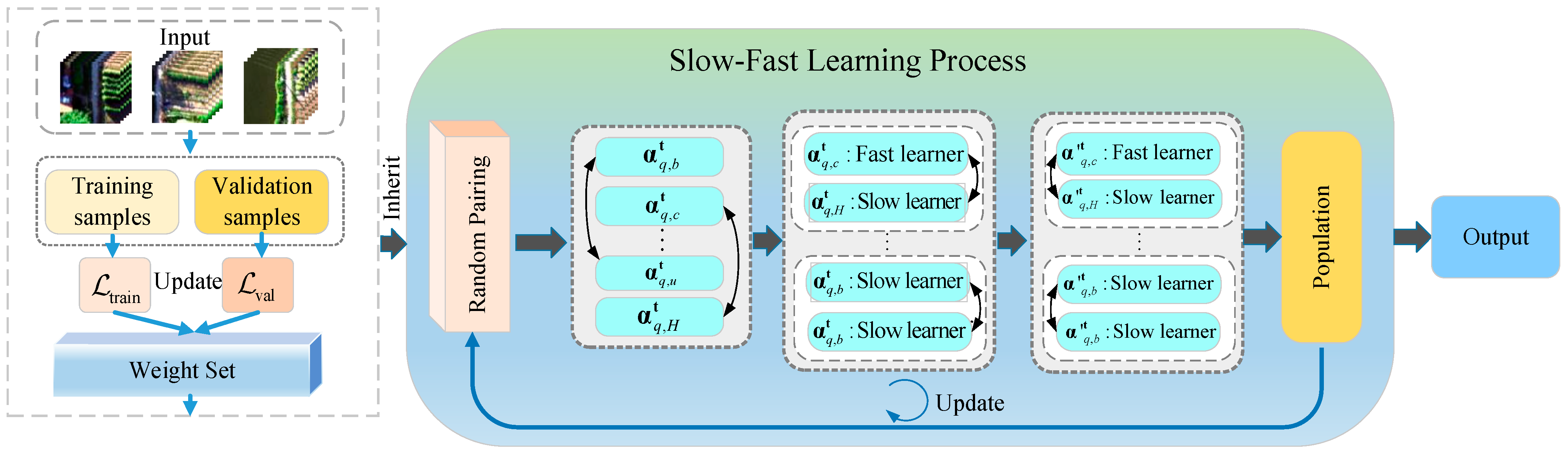Therefore, the slow–fast learning is essentially the optimizer for $\alpha$ parameters in our NAS. Specifically, we give the architecture vector ${\alpha }^t$ obtained by slow–fast learning in the t^th generation, and its iterative update method is shown in Figure 4.

$${\alpha }^{t+1}={\alpha }^t+\Delta {\alpha }^t$$

(11)

where the above equation satisfies ${ℒ}_{val}(C_{{\alpha }^{g+1}},w_{{\alpha }^{g+1}}^{*})<{ℒ}_{val}(C_{{\alpha }^g},w_{{\alpha }^g}^{*})$.

To generate pseudo gradient $\Delta {\alpha }^t$ effectively, this approach suggests utilizing a population of H architecture vectors ${\left\{\alpha \right\}}_{h=1}^H$. Each generation randomly splits the population into H/2 pairs. Next, for each pair of population q, the order of validation loss values is employed to identify the fast learner ${\alpha }_{q,f}^t$ and slow learner ${\alpha }_{q,s}^t$, with smaller loss values indicating slow learner and larger loss values indicating fast learner [${ℒ}_{val}(C_{{\alpha }_{q,f}^t},w_{{\alpha }_{q,f}^t}^{*})<{ℒ}_{val}(C_{{\alpha }_{q,s}^t},w_{{\alpha }_{q,s}^t}^{*})$]. Then, ${\alpha }_{q,s}^t$ learns from ${\alpha }_{q,f}^t$ and updates it.

$$\begin{array}{l}\Delta {\alpha }_{q,s}^t={\eta }_1({\alpha }_{q,f}^t-{\alpha }_{q,s}^t)+{\eta }_2\Delta {\alpha }_{q,s}^{t-1}\\ \end{array}$$

(12)

Here, ${\eta }_1,{\eta }_2\in [0,1]$ represents a randomly generated value obtained from a uniform distribution. Specifically, ${\eta }_1$ determines the step size for ${\alpha }_{q,s}^t$ to learn from ${\alpha }_{q,f}^t$, and ${\eta }_2$ determines the influence of momentum $\Delta {\alpha }_{q,s}^{t-1}$. Finally, all fast–slow learners are aggregated to form a new group of the t + 1th generation. The above pseudo gradient update method is derived from the second derivative of gradient descent in back propagation, so each architecture vector in the search space of the multi-attention mechanism designed in this work will move towards the optimal update direction from the vector that converges faster than them.

After the architecture update process, it is necessary to evaluate the performance of candidate architectures for decoding architecture vectors, so that for each pair of architecture vectors, fast learners can learn and update slow learners by verifying the loss. Subsequently, the candidate architecture $C_{{\alpha }^g}$ is assessed by solving the following optimization problems:

$$w_{{\alpha }^g}^{*}=\mathrm{optimize}(w_{{\alpha }^g})=step(step(\dots step(w_{{\alpha }^g}|C_{{\alpha }^g})\dots |C_{{\alpha }^g})|C_{{\alpha }^g})$$

(13)

In the given equation, $w_{a^g}^{*}$ represents the optimal weight of the candidate architecture, while $step(\cdot )$ denotes the iterative optimization process utilized for updating the weights of the neural network.

2.2.3. Lion Optimizer

The optimizer is utilized to update and compute the network parameters that influence model training and output, with the goal of approaching or achieving the optimal value and thereby minimizing (or maximizing) the loss function. This study utilizes the Lion optimizer, known for its simplicity, efficiency, and speed. Reducing redundancy is an important aspect of this work. At the same time, this optimizer is suitable for large-scale optimization problems involving big datasets or high-dimensional parameter spaces. The use of the Lion optimizer can not only effectively improve the accuracy of HSI data classification but also reduce memory overhead and effectively reduce training time because the algorithm only tracks momentum and uses symbolic operation to calculate updates. The Lion optimizer formula is written as follows [43]:

$${\theta }_{t+1}={\omega }_t{\theta }_t$$

(14)

$$g_t={\nabla }_{\theta }f({\theta }_{t-1})$$

(15)

where ${\omega }_t$ is the decay rate, ${\theta }_t$ is the weights, and $g_t={\nabla }_{\theta }f({\theta }_{t-1})$ is the gradient at ${\theta }_{t-1}$.

To calculate the average attenuation of the current and past square gradient, the mathematical relationship can be written as follows:

$$c_t={\beta }_1{m}_{t-1}+(1-{\beta }_1)g_t$$

(16)

where $c_t$ is the 1st moment estimate, and $m_{t-1}$ represents the momentum vector from the previous iteration. ${\beta }_1$ is the decay rate of the 1st moment. The weight reduction process for decoupling is as follows:

$${\theta }_t\leftarrow {\theta }_{t-1}-{\eta }_t(sign(ct)+\lambda {\theta }_{t-1})$$

(17)

where ${\eta }_t$ is the step size. To counteract biases, the bias-corrected first and second moments are computed in the following manner:

$$m_t\leftarrow {\beta }_2{m}_{t-1}+(1-{\beta }_2)g_t$$

(18)

The algorithm differs from various adaptive algorithms in that it only tracks momentum and uses symbolic operations to compute updates, leading to lower memory overhead and achieving a unified update magnitude across all dimensions.

3. Results

3.1. Hyperspectral Image Datasets

To assess the efficacy of the proposed NAS method, this research conducts classification experiments on three datasets: one standard hyperspectral dataset (Pavia University) and two practical datasets (Xuzhou and WHU-Hi-Hanchuan).

Table 2. Pavia University Dataset Labeled Sample Counts.

No.	Class	Color	Sample Numbers	False Color Map	Ground Truth Map
1	Asphalt		6631
2	Meadows		18,649
3	Gravel		2099
4	Trees		3064
5	Painted metal sheets		1345
6	Bare Soil		5029
7	Bitumen		1330
8	Self-Blocking Bricks		3682
9	Shadows		947
Total			42,776

,

Table 3. Xuzhou Dataset Labeled Sample Counts.

No.	Class	Color	Sample Numbers	False Color Map	Ground Truth Map
1	Bareland-1		26,396
2	Lakes		4027
3	Coals		2783
4	Cement		5214
5	Crops-1		13,184
6	Trees		2436
7	Bareland-2		6990
8	Crops-2		4777
9	Red-tiles		3070
Total			68,877

and

Table 4. WHU-Hi-Hanchuan Dataset Labeled Sample Counts.

No.	Class	Color	Sample Numbers	False Color Map	Ground Truth Map
1	Strawberry		44,735
2	Cowpea		22,753
3	Soybean		10,287
4	Sorghum		5353
5	Water spinach		1200
6	Watermelon		4533
7	Greens		5903
8	Trees		17,978
9	Grass		44,735
10	Red roof		9469
11	Gray roof		10,516
12	Plastic		16,911
13	Bare soil		3679
14	Road		9116
15	Bright object		18,560
16	Water		1136
Total			0

show the number of pixels in each category, the false color composite image, and the ground truth map of the three datasets, respectively. The aim is to reduce redundancy in the experiments and ensure a comprehensive evaluation. The Pavia University dataset was gathered using AROSIS sensors that flew over Pavia in northern Italy. It consists of 103 spectral bands and has a dataset size of 610 × 340 pixels. It consists of nine categories. The Xuzhou dataset was collected in November 2014 using the HySpex SWIR-384 and HySpex VNIR-1600 imaging spectrometers. The dataset consists of 436 bands and covers a specific pixel size in the mining area. A field survey was conducted, and a total of nine categories were calibrated. In total, 68,877 marker samples were used.

The WHU-Hi-Hanchuan dataset was collected in Hanchuan, Hubei Province, using the 17 mm focus Headwall Nano Hyperspec sensor installed on the Leica Airbot X6 UAV V1 platform. The size of the dataset is 1217 × 303 pixels, with 16 categories. The survey collected data from 68,877 marker samples.

3.2. Implementation Details

Our experiments are conducted at Intel (R) Xeon (R) 4208 [email protected] Processor and Nvidia GeForce RTX 2080Ti graphics card. We conducted 10 experiments to take the average value to obtain the overall accuracy (OA), average accuracy (AA), and Kappa coefficient (K) of the experiment.

The hyperspectral image samples are extracted using the sliding window strategy with a window size and overlap rate set at 50%. For training purposes, 30 samples are randomly selected as the training dataset, while 20 samples are used for validation. The training dataset is utilized to train the weights and biases of each neuron in the model, whereas the architecture variables are optimized based on the validation dataset. Once the optimal architecture is obtained, the remaining samples are employed as the test dataset to evaluate the performance of the optimized network architecture and derive the final classification results.

To evaluate the discovered architectures, we conducted evaluations on the discovered architectures with two cells and sixteen initial channels. Each cell consisted of seven nodes, including two input nodes, four intermediate nodes, and one output node. The population size (N) and generation number were set to 1, 20, 35, and 50, respectively. The batch size for each search stage was 32, and we used Stochastic Gradient Descent (SGD) to optimize the weight parameters with a learning rate of 0.025. The cosine power annealing strategy was employed to reduce the learning rate, with a maximum learning rate of 0.025, a minimum learning rate of 0.0001, and a power curve parameter of 2. To prevent overfitting and ensure the robustness of the final model, we also used label smoothing regularization with a smoothing factor of 0.1.

3.3. Classification Comparison with State-of-the-Art Methods

In this section, we evaluate the classification performance of MS³ANAS by comparing it with several advanced methods. These methods include Extended Morphological Profile combined with Support Vector Machine (EMP-SVM) [44], 2D-CNN [11], 3D-CNN [14], Spectral–Spatial Residual Network (SSRN) [16], Residual Network (ResNet) [45], Multi-Layer Perceptron Mixer (MLP Mixer) [46], CNN model designed using NAS (CNAS) [34], and Efficient Convolutional Neural Architecture Search for LiDAR DSM Classification (AN-AS-CPA-LS) [47]. To ensure the rigor of the experiment, we randomly selected three training samples for classes with fewer than three samples. The training times for manually designed CNN models were set to 200. For CNAS and ANAS-CPA-LS, they searched for the optimal architecture based on the DARTS strategy. Therefore, their configuration and superparameter settings were the same as those of the MS³ANAS model. All experimental results are shown in

Table 5. Classification results of all methods on the Pavia University dataset.

Methods	EMP-SVM	2D-CNN	3D-CNN	SSRN	MLP-Mixer	CNAS	ANAS-CPA-LS	MS3ANAS
1	60.77 ± 9.11	76.52 ± 7.32	86.51 ± 3.50	94.01 ± 0.72	96.17 ± 1.07	96.45 ± 0.13	97.70 ± 0.70	99.01 ± 0.35
2	95.68 ± 1.10	94.47 ± 3.35	94.32 ± 3.69	99.40 ± 0.22	97.80 ± 0.81	98.96 ± 0.02	99.46 ± 0.42	99.79 ± 0.14
3	88.06 ± 6.64	93.23 ± 0.13	69.58 ± 5.82	98.26 ± 3.28	94.43 ± 3.16	98.17 ± 0.11	91.13 ± 6.27	97.09 ± 0.11
4	98.38 ± 1.55	99.52 ± 0.15	95.97 ± 3.02	98.73 ± 1.32	99.31 ± 1.00	99.70 ± 0.04	99.66 ± 0.16	99.89 ± 0.01
5	99.46 ± 0.36	99.36 ± 0.63	99.58 ± 0.11	99.64 ± 0.69	99.78 ± 0.33	99.42 ± 0.04	100 ± 0.00	99.87 ± 0.12
6	92.70 ± 1.16	81.95 ± 12.16	94.80 ± 1.00	95.28 ± 0.19	99.27 ± 4.13	99.00 ± 0.21	99.80 ± 0.11	99.86 ± 0.07
7	99.77 ± 0.22	42.66 ± 9.32	95.07 ± 1.29	96.35 ± 0.35	98.47 ± 0.53	99.41 ± 0.13	99.16 ± 0.83	99.38 ± 0.36
8	65.37 ± 6.31	71.28 ± 5.13	84.52 ± 6.71	84.58 ± 0.03	81.86 ± 2.72	86.12 ± 0.25	95.13 ± 0.68	95.33 ± 1.33
9	49.30 ± 8.33	96.79 ± 2.22	99.77 ± 0.10	99.74 ± 0.16	99.93 ± 1.46	97.47 ± 1.33	99.65 ± 0.34	100 ± 0.00
OA/%	83.39 ± 0.85	87.36 ± 1.67	91.04 ± 1.70	94.68 ± 1.32	96.16 ± 0.71	97.42 ± 0.29	98.44 ± 0.57	99.16 ± 0.03
AA/%	83.27 ± 3.86	89.14 ± 7.20	91.12 ± 1.11	96.22 ± 1.58	96.32 ± 0.90	97.18 ± 0.25	97.97 ± 0.72	98.91 ± 1.14
100 K	81.70 ± 1.44	82.99 ± 2.46	87.99 ± 2.35	92.94 ± 0.41	94.89 ± 0.09	96.76 ± 0.18	97.93 ± 0.76	98.89 ± 0.09
Params/M	0.0032	0.1439	0.0934	0.0894	0.4305	0.2164	0.2432	0.1376
Flops/G	0.0008	0.1274	0.4682	0.4843	0.0248	2.8302	2.7284	0.0194

,

Table 6. Classification results of all methods on the Xuzhou dataset.

Methods	EMP-SVM	2D-CNN	3D-CNN	SSRN	MLP-Mixer	CNAS	ANAS-CPA-LS	MS3ANAS
1	95.60 ± 1.46	85.83 ± 1.83	94.71 ± 0.80	95.55 ± 1.92	96.33 ± 0.06	98.86 ± 0.66	99.15 ± 0.65	99.71 ± 0.13
2	92.32 ± 0.04	90.94 ± 4.72	85.10 ± 1.34	94.87 ± 4.97	99.94 ± 0.61	99.06 ± 0.79	99.50 ± 0.49	99.94 ± 0.03
3	85.76 ± 0.82	82.38 ± 1.81	92.21 ± 0.06	89.04 ± 6.99	93.98 ± 0.44	95.09 ± 2.71	99.40 ± 0.03	99.99 ± 0.01
4	98.45 ± 1.57	93.67 ± 4.81	96.86 ± 0.37	95.68 ± 0.28	95.02 ± 3.02	92.82 ± 5.03	99.10 ± 0.16	99.91 ± 0.04
5	88.00 ± 0.09	97.30 ± 0.82	93.33 ± 1.74	92.88 ± 0.37	96.20 ± 0.93	98.57 ± 0.15	95.95 ± 0.01	94.21 ± 0.62
6	82.41 ± 0.24	83.66 ± 2.10	86.41 ± 1.36	95.28 ± 1.26	79.38 ± 6.11	91.75 ± 4.89	97.56 ± 0.24	97.55 ± 0.45
7	72.46 ± 3.52	90.16 ± 3.11	86.47 ± 2.43	90.08 ± 1.23	92.75 ± 3.05	96.40 ± 1.41	94.83 ± 0.15	99.86 ± 0.98
8	59.38 ± 2.77	96.93 ± 1.80	98.81 ± 1.04	95.95 ± 0.45	89.20 ± 8.11	99.60 ± 0.24	97.07 ± 2.06	99.72 ± 0.07
9	92.16 ± 1.26	89.71 ± 0.32	89.72 ± 0.35	89.77 ± 2.49	98.27 ± 0.32	98.51 ± 0.58	96.92 ± 0.07	99.92 ± 0.01
OA/%	84.50 ± 0.81	88.32 ± 0.27	91.71 ± 0.93	92.41 ± 1.34	94.54 ± 2.32	97.07 ± 0.06	97.72 ± 0.19	98.44 ± 1.67
AA/%	85.17 ± 1.30	87.84 ± 0.72	91.51 ± 1.84	92.90 ± 2.21	93.45 ± 2.51	96.74 ± 1.82	97.67 ± 0.49	98.98 ± 0.25
100 K	80.38 ± 0.77	84.87 ± 0.43	89.46 ± 1.31	90.37 ± 1.66	93.14 ± 2.89	97.04 ± 1.01	97.11 ± 0.23	98.04 ± 2.10
Params/M	0.0193	0.0627	0.1094	0.2761	0.3976	0.3844	0.2452	0.0598
Flops/G	0.0059	0.1354	0.4717	0.4489	0.0643	3.0262	2.6810	0.0198

and

Table 7. Classification results of all methods on the WHU-Hi-Hanchuan dataset.

Methods	EMP-SVM	2D-CNN	3D-CNN	SSRN	MLP-Mixer	CNAS	ANAS-CPA-LS	MS3ANAS
1	85.45 ± 2.47	88.15 ± 0.32	87.16 ± 0.19	90.11 ± 1.52	91.62 ± 2.63	93.71 ± 0.13	95.93 ± 0.68	97.99 ± 0.31
2	92.05 ± 2.01	87.90 ± 3.17	93.69 ± 0.01	94.31 ± 2.52	95.14 ± 0.01	96.32 ± 0.25	98.23 ± 0.23	98.68 ± 0.14
3	80.76 ± 3.53	82.11 ± 0.05	87.66 ± 1.09	90.52 ± 1.77	90.47 ± 0.32	94.41 ± 1.22	96.09 ± 2.92	98.80 ± 0.14
4	93.03 ± 2.77	86.44 ± 1.56	92.53 ± 1.23	97.82 ± 0.16	97.47 ± 0.70	97.97 ± 0.49	99.44 ± 0.04	99.32 ± 0.12
5	77.85 ± 16.59	52.13 ± 3.19	61.44 ± 4.24	81.64 ± 5.60	78.18 ± 3.02	88.30 ± 4.50	89.75 ± 2.39	96.02 ± 1.44
6	64.54 ± 7.93	65.71 ± 1.61	75.41 ± 1.09	74.34 ± 1.91	84.51 ± 0.05	84.48 ± 1.65	91.86 ± 0.68	94.00 ± 0.01
7	65.95 ± 1.24	69.80 ± 6.17	74.36 ± 1.63	82.13 ± 0.78	82.35 ± 3.44	84.44 ± 5.14	92.51 ± 2.64	93.79 ± 2.94
8	88.62 ± 0.49	83.48 ± 0.82	90.43 ± 2.19	92.07 ± 1.12	91.39 ± 1.05	95.86 ± 0.71	98.35 ± 0.02	98.15 ± 0.13
9	75.43 ± 5.81	78.55 ± 1.34	87.84 ± 1.25	87.51 ± 2.47	88.69 ± 3.05	90.85 ± 2.13	94.88 ± 0.87	97.35 ± 0.38
10	90.48 ± 3.12	93.35 ± 1.26	95.38 ± 1.69	95.04 ± 0.44	95.66 ± 2.72	97.38 ± 1.22	99.22 ± 0.04	99.73 ± 0.19
11	85.60 ± 3.01	82.62 ± 0.85	89.71 ± 1.26	86.97 ± 2.67	91.47 ± 1.37	91.39 ± 0.02	96.60 ± 0.01	97.53 ± 0.07
12	73.08 ± 2.90	74.78 ± 1.89	75.03 ± 4.91	80.84 ± 0.69	86.70 ± 0.89	89.59 ± 3.92	93.69 ± 0.19	94.75 ± 0.33
13	67.30 ± 1.71	67.97 ± 2.68	81.14 ± 1.10	88.13 ± 2.92	85.28 ± 1.08	87.45 ± 5.35	94.50 ± 1.87	95.55 ± 0.26
14	85.91 ± 0.73	84.59 ± 2.78	89.09 ± 0.13	92.72 ± 1.08	89.45 ± 0.85	94.22 ± 2.02	97.32 ± 0.23	97.47 ± 0.93
15	88.87 ± 6.20	87.60 ± 2.66	89.78 ± 4.21	84.40 ± 11.6	90.09 ± 7.58	92.99 ± 0.15	97.08 ± 0.56	95.82 ± 0.71
16	97.72 ± 3.02	97.48 ± 0.71	97.79 ± 0.26	99.15 ± 0.16	99.11 ± 0.01	99.49 ± 1.37	99.66 ± 0.14	99.77 ± 0.06
OA/%	87.96 ± 0.30	89.07 ± 0.31	91.01 ± 0.34	92.78 ± 0.09	93.95 ± 0.02	96.15 ± 0.03	97.44 ± 0.03	98.30 ± 0.07
AA/%	82.04 ± 3.97	83.04 ± 2.45	85.53 ± 0.44	88.61 ± 1.24	89.66 ± 0.98	94.43 ± 1.07	95.50 ± 0.44	97.17 ± 0.25
100 K	85.85 ± 0.37	87.85 ± 0.36	89.43 ± 0.40	91.53 ± 0.11	91.73 ± 0.03	95.32 ± 0.02	96.97 ± 0.08	98.01 ± 0.08
Params/M	0.0170	0.0677	0.9028	1.0653	0.6211	0.3807	0.3672	0.1564
Flops/G	0.0009	0.1466	0.4719	0.4780	0.1035	3.9640	4.0821	0.0742

, and they represent the average values of ten runs with different random initializations.

As shown in Table 5, Table 6 and Table 7, our proposed MS³ANAS typically outperforms other methods in terms of OA, AA, and Kappa on three datasets. The EMP-SVM has the lowest classification accuracy, and the classification accuracy of 2D-CNN and 3D-CNN is also poor, while SSRN uses skip connections to extract depth feature information, resulting in higher classification accuracy than 2D-CNN or 3D-CNN. This is due to the lightweight spatial–spectral attention operations found in multi-scale attention search spaces that can better extract joint spectral–spatial features of hyperspectral images. Taking the Pavia dataset as an example, compared to CNAS, the MS³ANAS model proposed in this paper improves OA from 97.42% to 99.16%. Both ANAS-CPA-LS and MS³ANAS have built the search space of attention mechanism, but the search space built by our method contains attention mechanisms of multiple scales. At the same time, we use small filters to reduce parameters while maintaining a large range of receptive fields. Therefore, the ability to extract different scales of spectral–spatial features from data is enhanced, thereby improving classification performance. However, in the case of limited training samples, the ability of attention mechanisms to fit spatial structural information is not easily utilized. Compared with ANAS-CPA-LS, MS³ANAS has better classification performance.

As shown in Table 6, compared with EMP-SVM, 2D-CNN, 3D-CNN, SSRN, ResNet, CNAS, and ANAS-CPA-LS, OA obtained by our proposed method increased by 13.94%, 10.12%, 6.73%, 6.03%, 3.90%, 1.37%, and 0.72%, respectively, on the Xuzhou dataset. Taking the WHU-Hi-Hanchuan dataset as an example, OA reached 98.30%, and increased by 0.86%, 2.15%, 4.35%, 5.52%, 7.29%, 9.23%, and 10.34%, respectively, compared with ANAS-CPA-LS, CNAS, ResNet, SSRN, 3D-CNN, 2D-CNN, and EMP-SVM. Except for EMP-SVM, 2D-CNN is the second worst in performance because it only uses spatial features. Meanwhile, for other methods, MS³ANAS achieved significant improvements in both AA and Kappa results. From the classification results of the three datasets, it can be seen that the overall performance of the NAS-based method is higher than that of the handmade methods. At the same time, the search space using a multi-scale attention mechanism can enhance the model’s ability to consider spectral and spatial information, effectively improving classification performance.

Due to the design of a lightweight NAS model in this article, we compared its complexity with existing technologies in terms of required model parameters (Params) and Flops. We can see from Table 5, Table 6 and Table 7 that different search space operations and architecture update methods can lead to differences in the amount of network parameters. Flops are determined by the input data size and parameters; therefore, we will conduct an overall analysis based on the complexity and classification performance of the network model. Compared with handmade hyperspectral image classification models such as 2D-CNN and 3D-CNN, as well as NAS methods such as CNAS and ANAS-CPA-LS, the proposed method has lower occupancy rates in Params and Flops but achieves the highest OA while achieving the best classification performance on three datasets. The results further indicate that the proposed method can solve classification tasks with low cost but high performance. This mainly benefits from the effectiveness of our special multi-scale search space and the applicability of the slow–fast learning architecture update paradigm to different hyperspectral datasets.

The classification diagrams of the other seven methods on the three HSI datasets are displayed in Figure 5, Figure 6 and Figure 7. It is evident that the proposed algorithm demonstrates superior performance in general. Compared with ANAS-CPA-LS, the ANAS-CPA-LS incorrectly classified Bare Soil (Class 6) as Meadows (Class 2) in Figure 5h of the Pavia dataset classification results.

In Figure 6h of the experimental results on the Xuzhou dataset, some Coals (level 2) were mistakenly classified as Cement (level 7). Through a comparison of the classification maps obtained, it can be concluded that our method achieves more accurate classification results with reduced salt-and-pepper noise. Because our method uses the combination of multi-scale attention mechanism and common attention mechanism as the search operator, it can more effectively extract deeper spatial features and combine spectral and spatial information to capture more complex and abstract features.

4. Discussion

4.1. Optimal Architecture Analysis

Figure 8, Figure 9 and Figure 10 illustrate the cells with the optimal architecture on the three datasets, which are obtained through the proposed method. These cells consist of both normal cells and reduction cells.

In our experiment, we employed the slow–fast learning paradigms and the multi-scale attention mechanism search space to search for the optimal network architecture for each HSI dataset. We can observe that the network architecture retains more multi-scale search operators (such as MCS_ sepConv (3 × 3), MCS_ SepConv (5 × 5), and MCS_ SepConv (7 × 7)). As a result, our model comprises a higher number of learnable parameters, allowing it to maintain a wide range of receptive fields. This effectively addresses the issues of gradient disappearance and network degradation. Consequently, our method can extract scaled spectral–spatial features from the data more effectively, leading to an improvement in classification performance.

4.2. The Analysis of Slow and Fast Learning Using Optimal Combination Actions

In order to empirically analyze the slow–fast learning process, it is necessary to select different parameters for experiments. In this section, the generation is combined with different search spaces to conduct experiments on three datasets. In the experiment, the control variable method is used for each dataset. The number of experiments, training samples, validation samples, and test samples is consistent. The conclusion drawn is that the (a) Pavia University, (b) Xuzhou, and (c) WHU-Hi-Hanchuan datasets display the complete presentation of each combination, and all datasets display MA + MS and generation 50 as the best performance combination (Figure 11). Therefore, it can be proven that slow–fast learning can perform pseudo gradient architecture updates on different hyperspectral imbalanced data during the construction process of building units, effectively improving classification performance.

4.3. Ablation Experiments Analysis

To validate the effectiveness of our method in HSI data classification, we conducted numerous ablation experiments, as presented in

Table 8. The classification results of all methods on each dataset.

Dataset	Index	CNAS	MS + NAS	SF + MSNAS	SF + MSNAS + Lion
Pavia University	OA (%)	97.42 ± 0.29	97.90 ± 0.37	98.92 ± 0.20	99.16 ± 0.03
	AA (%)	97.18 ± 0.25	97.84 ± 1.36	98.07 ± 1.83	98.91 ± 1.14
	100 K	96.76 ± 0.18	97.95 ± 0.79	98.45 ± 2.51	98.89 ± 0.09
	Search Cost (hours)	3.054	3.013	2.982	2.733
	Params (M)	0.1692	0.1574	0.1579	0.1564
Xuzhou	OA (%)	97.07 ± 0.06	97.84 ± 0.94	98.23 ± 0.09	98.44 ± 1.67
	AA (%)	96.74 ± 1.82	97.94 ± 0.81	98.70 ± 0.59	98.98 ± 0.25
	100 K	97.04 ± 1.01	97.18 ± 0.78	97.84 ± 0.42	98.04 ± 2.10
	Search Cost (hours)	3.312	3.295	3.205	3.094
	Params (M)	0.0658	0.0570	0.0578	0.059
WHU-Hi-Hanchuan	OA (%)	96.15 ± 0.03	97.04 ± 0.94	97.93 ± 0.09	98.30 ± 0.07
	AA (%)	94.43 ± 1.07	96.52 ± 0.81	97.01 ± 0.59	97.17 ± 0.25
	100 K	95.32 ± 0.02	96.11 ± 0.78	97.74 ± 0.42	98.01 ± 0.08
	Search Cost (hours)	4.201	4.178	4.113	4.026
	Params (M)	0.292	0.174	0.176	0.156

. Specifically, when we solely employ the CNAS model for classifying the Pavia dataset with only 30 training samples, OA reached 97.42%, 97.07%, and 96.15%, respectively. When CNAS was combined with multi-scale attention expansion mechanism search space (MS), OA increased by 0.48%, 0.77%, and 0.89%, respectively. This result demonstrates that the incorporation of a multi-scale attention mechanism to expand the search space enhances the network’s sensitivity to informative features, resulting in a slight improvement in the classification performance of the model. In comparison to CNAS, our method achieves better results. the search time of MS + NAS on the three datasets does not change significantly, but it significantly reduces the parameters and achieves better classification accuracy. Obviously, when NAS was combined with the slow–fast learning paradigm search strategy, the OA of the three datasets increased by 1.02%, 0.39%, and 0.89%, respectively. This is due to the application of slow and fast learning paradigms to optimize and interactively update the architecture vector. It can update the architecture of different hyperspectral imbalanced data and obtain classification models with stronger generalization ability. At the same time, it can be observed that the search time for the three datasets was reduced by 0.249 h, 0.111 h, and 0.087 h after SF + MSNAS referenced the Lion optimizer. This is because this optimizer can effectively reduce the time consumption of NAS architecture search. In addition, the algorithm only tracks momentum, effectively reducing memory overhead.

5. Conclusions

In this paper, we introduce a neural network architecture search algorithm called MS³ANAS. This approach aims to address the limitations of conventional differentiable NAS methods in three key areas: search space, search strategy, and architecture resource optimization. Firstly, we introduce an extended search space with a multi-scale attention mechanism, which can not only enhance the robustness and receptive field capture ability of the model but also better realize path optimization. Secondly, we quoted the slow–fast architecture learning paradigm, which not only optimizes the iterative updating of architecture vectors but also effectively improves the model’s generalization ability. Finally, the Lion optimizer was introduced to improve the accuracy of HSI data classification, reduce memory overhead, and reduce computational complexity. We conducted experiments on three HSI datasets and compared MS³ANAS with seven methods. The experimental results show that our method is more competitive. Through the datasets of Xuzhou, Pavia University, and WHU-Hi-Hanchuan, the OA of our method reached 97.82%, 98.46%, and 98.41%, respectively.

In future work, we will further optimize the NAS structure continuously to make it more lightweight and easier to adapt to more complex remote sensing image classification tasks. Furthermore, it is important to consider the practical applicability of our proposed method. Meanwhile, we plan to apply our approach to real-world hyperspectral image classification tasks, such as environmental monitoring, agricultural assessment, and urban planning. By validating the performance of our method on these practical applications, we can demonstrate its effectiveness and potential impact in various domains. Moreover, the potential applications of our method extend beyond hyperspectral image classification. By exploring these new application areas, we can further broaden the scope of our research and contribute to advancements in related fields. We are excited about the opportunities that lie ahead and look forward to witnessing the practical implementation and impact of our work in the field of remote sensing and computer vision.

References

1. Transon, J.; d’Andrimont, R.; Maugnard, A.; Defourny, P. Survey ofhyperspectral earth observation applications from space in the sentinel-2 context. Remote Sens. 2018, 10, 157. [Google Scholar] [CrossRef]
2. Carrino, T.A.; Crósta, A.P.; Toledo, C.L.B.; Silva, A.M. Hyper-spectral remote sensing applied to mineral exploration in southern peru:A multiple data integration approach in the chapi chiara gold prospect. Int. J. Appl. Earth Obs. Geoinf. 2018, 64, 287–300. [Google Scholar]
3. Behmann, J.; Steinrücken, J.; Plümer, L. Detection of early plant stress responses in hyperspectral images. ISPRS J. Photogramm. Remote Sens. 2014, 93, 98–111. [Google Scholar] [CrossRef]
4. Shimoni, M.; Haelterman, R.; Perneel, C. Hypersectral imaging for military and security applications: Combining myriad processing and sensing techniques. IEEE Geosci. Remote Sens. Mag. 2019, 7, 101–117. [Google Scholar] [CrossRef]
5. Sun, W.; Peng, J.; Yang, G.; Du, Q. Fast and latent low-ranksubspace clustering for hyperspectral band selection. IEEE Trans. Geosci. Remote Sens. 2020, 58, 3906–3915. [Google Scholar] [CrossRef]
6. Samadzadegan, F.; Hasani, H.; Schenk, T. Simultaneous feature selection and SVM parameter determination in classification of hyperspectral imagery using Ant Colony Optimization. Can. J. Remote Sens. 2012, 38, 139–156. [Google Scholar] [CrossRef]
7. Chandra, B.; Sharma, R.K. On improving recurrent neural network for image classification. In Proceedings of the 2017 International Joint Conference on Neural Networks (IJCNN), Anchorage, AK, USA, 14–19 May 2017; pp. 1904–1907. [Google Scholar] [CrossRef]
8. Hu, W.; Huang, Y.; Wei, L.; Zhang, F.; Li, H. Deep convolutionalneural networks for hyperspectral image classification. J. Sens. 2015, 2015, 258619. [Google Scholar] [CrossRef]
9. Makantasis, K.; Karantzalos, K.; Doulamis, A.; Doulamis, N. Deep supervised learning for hyperspectral data classification through convolutional neural networks. In Proceedings of the 2015 IEEE International Geoscience and Remote Sensing Symposium (IGARSS), Milan, Italy, 26–31 July 2015; pp. 4959–4962. [Google Scholar]
10. Li, W.; Wu, G.; Zhang, F.; Du, Q. Hyperspectral Image Classification Using Deep Pixel-Pair Features. IEEE Trans. Geosci. Remote Sens. 2016, 55, 844–853. [Google Scholar] [CrossRef]
11. Yue, J.; Zhao, W.; Mao, S.; Liu, H. Spectral–spatial classification of hyperspectral images using deep convolutional neural networks. Remote Sens. Lett. 2015, 6, 468–477. [Google Scholar] [CrossRef]
12. Zhang, H.; Li, Y.; Zhang, Y.; Shen, Q. Spectral-spatial classification of hyperspectral imagery using a dual-channel convolutional neural network. Remote Sens. Lett. 2017, 8, 438–447. [Google Scholar] [CrossRef]
13. Wang, B.; Shao, Q.; Song, D.; Li, Z.; Tang, Y.; Yang, C.; Wang, M. A Spectral-Spatial Features Integrated Network for Hyperspectral Detection of Marine Oil Spill. Remote Sens. 2021, 13, 1568. [Google Scholar] [CrossRef]
14. Li, Y.; Zhang, H.; Shen, Q. Spectral–spatial classification of hyper-spectral imagery with 3d convolutional neural network. Remote Sens. 2017, 9, 67. [Google Scholar] [CrossRef]
15. Chen, Y.; Jiang, H.; Li, C.; Jia, X.; Ghamisi, P. Deep feature extraction and classification of hyperspectral images based on convolutional neural networks. IEEE Trans. Geosci. Remote Sens. 2016, 54, 6232–6251. [Google Scholar] [CrossRef]
16. Zhong, Z.; Li, J.; Luo, Z.; Chapman, M. Spectral–spatial residual network for hyperspectral image classification: A 3-d deep learning framework. IEEE Trans. Geosci. Remote Sens. 2018, 56, 847–858. [Google Scholar] [CrossRef]
17. Zhang, H.; Li, Y.; Jiang, Y.; Wang, P.; Shen, Q.; Shen, C. Hyperspectral classification based on lightweight 3-d-cnn with transfer learning. IEEE Trans. Geosci. Remote Sens. 2019, 57, 5813–5828. [Google Scholar] [CrossRef]
18. Yang, G.; Gewali, U.B.; Ientilucci, E.; Gartley, M.; Monteiro, S.T. Dual-Channel Densenet for Hyperspectral Image Classification. In Proceedings of the IGARSS 2018—2018 IEEE International Geoscience and Remote Sensing Symposium, Valencia, Spain, 22–27 July 2018; pp. 2595–2598. [Google Scholar]
19. Bagaskara, A.; Suryanegara, M. Evaluation of VGG-16 and VGG-19 Deep Learning Architecture for Classifying Dementia People. In Proceedings of the 2021 4th International Conference of Computer and Informatics Engineering (IC2IE), Depok, Indonesia, 14–15 September 2021; pp. 1–4. [Google Scholar]
20. Aswathy, P.; Siddhartha; Mishra, D. Deep GoogLeNet Features for Visual Object Tracking. In Proceedings of the 2018 IEEE 13th International Conference on Industrial and Information Systems (ICIIS), Rupnagar, India, 1–2 December 2018; pp. 60–66. [Google Scholar]
21. Xia, M.; Yuan, G.; Yang, L.; Xia, K.; Ren, Y.; Shi, Z.; Zhou, H. Few-Shot Hyperspectral Image Classification Based on Convolutional Residuals and SAM Siamese Networks. Electronics 2023, 12, 3415. [Google Scholar] [CrossRef]
22. Jiang, Y.; Yu, S.; Wang, T.; Sun, Z.; Wang, S. Skeleton-Based Human Action Recognition Based on Single Path One-Shot Neural Architecture Search. Electronics 2023, 12, 3156. [Google Scholar] [CrossRef]
23. Xu, H.; Yao, L.; Li, Z.; Liang, X.; Zhang, W. Auto-FPN: Auto-matic network architecture adaptation for object detection beyond classification. In Proceedings of the IEEE/CVF International Conference on Computer Vision (ICCV), Seoul, Republic of Korea, 27 October–2 November 2019; pp. 6648–6657. [Google Scholar]
24. Zoph, B.; Le, Q.V. Neural architecture search with reinforcement earning. In Proceedings of the International Conference on Learning Representations, Toulon, France, 24–26 April 2017; pp. 1–16. [Google Scholar]
25. Real, E.; Aggarwal, A.; Huang, Y.; Le, Q.V. Regularized evolution for image classifier architecture search. In Proceedings of the Association for the Advancement of Artificial Intelligence, Honolulu, HI, USA, 27 January–1 February 2019; pp. 4780–4789. [Google Scholar]
26. Tan, M.; Chen, B.; Pang, R.; Vasudevan, V.; Sandler, M.; Howard, A.; Le, Q.V. MnasNet: Platform-Aware neural architecture search for mobile. In Proceedings of the IEEE/CVF Conference on Computer Vision and Pattern Recognition (CVPR), Long Beach, CA, USA, 15–20 June 2019; pp. 2820–2828. [Google Scholar]
27. Jin, J.; Zhang, Q.; He, J.; Yu, H. Quantum Dynamic Optimization Algorithm for Neural Architecture Search on Image Classification. Electronics 2022, 11, 3969. [Google Scholar] [CrossRef]
28. Liu, H.; Simonyan, K.; Yang, Y. DARTS: Differentiable architecture search. In Proceedings of the International Conference on Learning Representations, New Orleans, LA, USA, 30 April–30 May 2019; pp. 1–13. [Google Scholar]
29. Stanley, K.O.; Clune, J.; Lehman, J.; Miikkulainen, R. Designing neural networks through neuroevolution. Nat. Mach. Intell. 2019, 1, 24–35. [Google Scholar] [CrossRef]
30. Real, E.; Moore, S.; Selle, A.; Saxena, S.; Suematsu, Y.L.; Tan, J.; Le, Q.V.; Kurakin, A. Large-scale evolution of image classififiers. In Proceedings of the 34th International Conference on Machine Learning, PMLR, Sydney, NSW, Australia, 6–11 August 2017; pp. 2902–2911. [Google Scholar]
31. Liang, H.; Zhang, S.; Sun, J.; He, X.; Huang, W.; Zhuang, K.; Li, Z. DARTS+: Improved differentiable architecture search with early stopping. arXiv 2020, arXiv:1909.06035. [Google Scholar]
32. Guo, Z.; Zhang, X.; Mu, H.; Heng, W.; Liu, Z.; Wei, Y.; Sun, J. Single path one-shot neural architecture search with uniform sampling. In Proceedings of the Computer Vision–ECCV 2020: 16th European Conference, Glasgow, UK, 23–28 August 2020; Volume 12361, pp. 544–560. [Google Scholar] [CrossRef]
33. Park, G.; Yi, Y. CondNAS: Neural Architecture Search for Conditional CNNs. Electronics 2022, 11, 1101. [Google Scholar] [CrossRef]
34. Stanley, K.O.; Miikkulainen, R. Evolving neural networks through augmenting topologies. Evol. Comput. 2002, 10, 99–127. [Google Scholar] [CrossRef] [PubMed]
35. Chen, Y.; Zhu, K.; Zhu, L.; He, X.; Ghamisi, P.; Benediktsson, J.A. Automatic design of convolutional neural network for hyperspectral image classification. IEEE Trans. Geosci. Remote Sens. 2019, 57, 7048–7066. [Google Scholar] [CrossRef]
36. Hu, J.; Shen, L.; Sun, G. Squeeze–and–excitation networks. In Proceedings of the IEEE Conference on Computer Vision and Pattern Recognition (CVPR), Salt Lake City, UT, USA, 18–23 June 2018; pp. 7132–7141. [Google Scholar]
37. Roy, S.K.; Manna, S.; Song, T.; Bruzzone, L. Attention-Based Adaptive Spectral–Spatial Kernel ResNet for Hyperspectral Image Classification. IEEE Trans. Geosci. Remote Sens. 2020, 59, 7831–7843. [Google Scholar] [CrossRef]
38. Woo, S.; Park, J.; Lee, J.Y.; Kweon, I.S. CBAM: Convolutional Block Attention Module. In Proceedings of the European Conference on Computer Vision, Munich, Germany, 8–14 September 2018. [Google Scholar]
39. Misra, D.; Nalamada, T.; Arasanipalai, A.U.; Hou, Q. Rotate to Attend: Convolutional Triplet Attention Module. In Proceedings of the IEEE Winter Conference on Applications of Computer Vision, Waikoloa, HI, USA, 3–8 January 2021; pp. 3138–3147. [Google Scholar]
40. Hou, Q.; Zhou, D.; Feng, J. Coordinate Attention for Efficient Mobile Network Design. In Proceedings of the Computer Vision and Pattern Recognition, Beijing, China, 29 October–1 November 2021. [Google Scholar]
41. Cao, C.; Xiang, H.; Song, W.; Yi, H.; Xiao, F.; Gao, X. Lightweight Multiscale Neural Architecture Search with Spectral–Spatial Attention for Hyperspectral Image Classification. IEEE Trans. Geosci. Remote Sens. 2023, 61, 1–15. [Google Scholar] [CrossRef]
42. Tan, H.; Cheng, R.; Huang, S.; He, C.; Qiu, C.; Yang, F.; Luo, P. RelativeNAS: Relative Neural Architecture Search via Slow-Fast Learning. IEEE Trans. Neural Netw. Learn. Syst. 2021, 34, 475–489. [Google Scholar] [CrossRef]
43. Chen, X.; Liang, C.; Huang, D.; Real, E.; Wang, K.; Liu, Y.; Pham, H.; Dong, X.; Luong, T.; Hsieh, C.-J.; et al. Symbolic Discovery of Optimization Algorithms. arXiv 2023, arXiv:2302.06675. [Google Scholar]
44. Melgani, F.; Bruzzone, L. Classification of hyperspectral remote sensing images with support vector machines. IEEE Trans. Geosci. Remote Sens. 2004, 42, 1778–1790. [Google Scholar] [CrossRef]
45. Liu, X.; Meng, Y.; Fu, M. Classification Research Based on Residual Network for Hyperspectral Image. In Proceedings of the 2019 IEEE 4th International Conference on Signal and Image Processing (ICSIP), Wuxi, China, 19–21 July 2019; pp. 911–915. [Google Scholar]
46. He, X.; Chen, Y. Modifications of the Multi-Layer Perceptron for Hyperspectral Image Classification. Remote Sens. 2021, 13, 3547. [Google Scholar] [CrossRef]
47. Wang, A.; Xue, D.; Wu, H.; Gu, Y. Efficient Convolutional Neural Architecture Search for LiDAR DSM Classification. IEEE Trans. Geosci. Remote Sens. 2022, 60, 1–17. [Google Scholar] [CrossRef]
Figure 1. The overall framework of the proposed MS3ANAS model.
Electronics 12 03641 g001
Figure 2. Multiple attention mechanism search space (a) CBAM; (d) CA; (b) SE; (c) TA.
Electronics 12 03641 g002aElectronics 12 03641 g002b
Figure 3. Multi-scale attention mechanism guided search space (a) MCS_sepConv(3 × 3); (b) MCS_sepConv(5 × 5); (c) MCS_sepConv(7 × 7).
Electronics 12 03641 g003
Figure 4. The slow–fast learning process.
Electronics 12 03641 g004
Figure 5. The classification results of the Pavia University dataset. (a) Ground truth map; (b) EMP-SVM; (c) 2D-CNN; (d)3D-CNN; (e) SSRN; (f) MLP-Mixer; (g) CNAS; (h) ANAS-CPA-LS; and (i) MS3ANAS.
Electronics 12 03641 g005
Figure 6. The classification results of the Xuzhou dataset. (a) Ground truth map; (b) EMP-SVM; (c) 2D-CNN; (d) 3D-CNN; (e) SSRN; (f) MLP-Mixer; (g) CNAS; (h) ANAS-CPA-LS; and (i) MS3ANAS.
Electronics 12 03641 g006
Figure 7. The classification results of the WHU-Hi-Hanchuan dataset. (a) Ground truth map; (b) EMP-SVM; (c) 2D-CNN; (d) 3D-CNN; (e) SSRN; (f) MLP-Mixer; (g) CNAS; (h) ANAS-CPA-LS; and (i) MS3ANAS.
Electronics 12 03641 g007
Figure 8. The searched cell architectures of the Pavia University dataset.
Electronics 12 03641 g008
Figure 9. The searched cell architectures of the Xuzhou dataset.
Electronics 12 03641 g009
Figure 10. The searched cell architectures of the WHU-Hi-Hanchuan dataset.
Electronics 12 03641 g010
Figure 11. The optimal combined action of the search space and the number of generations for each dataset. (a) Pavia University; (b) Xuzhou; (c) WHU-Hi-Hanchuan.
Electronics 12 03641 g011