A Multi-Stage Adaptive Copy-Paste Data Augmentation Algorithm Based on Model Training Preferences

Abstract

Datasets play an important role in the field of object detection. However, the production of the dataset is influenced by objective environment and human subjectivity, resulting in class imbalanced or even long-tailed distribution in the datasets. At present, the optimization methods based on data augmentation still rely on subjective parameter adjustments, which is tedious. In this paper, we propose a multi-stage adaptive Copy-Paste augmentation (MSACP) algorithm. This algorithm divides model training into multiple training stages, each stage forming unique training preferences for that stage. Based on these training preferences, the class information of the training set is adaptively adjusted, which not only alleviates the problem of class imbalance in training, but also expands different sample sizes for categories with insufficient information at different training stages. Experimental verification of the traffic sign dataset Tsinghua–Tencent 100K (TT100K) was carried out and showed that the proposed method not only can improve the class imbalance in the dataset, but can also improve the detection performance of models. By using MSACP to transplant the trained optimal weights to an embedded platform, and combining YOLOv3-tiny, the model’s accuracy in detecting traffic signs in autonomous driving scenarios was improved, verifying the effectiveness of the MSACP algorithm in practical applications.

1. Introduction

The total number of different classes in the real world is different, which leads to the class imbalance of datasets when collecting data [1]. Currently, most competitive models rely on huge amounts of data for training. However, the large amount of data can lead to more extreme class imbalances; that is, a few classes have a very large sample size, while most classes have a small sample size. The sample size of the classes showed a long-tail distribution [2]. When the model is trained, it is easy to overfit the classes with insufficient samples.

Because datasets are too expensive to produce, researchers focus on algorithms to optimize datasets. Two common data processing methods for class imbalance are sample sampling and cost-sensitive learning. For the sample sampling technology, the main idea of this method is to directly change the feature distribution of the dataset by adding or deleting the sample size of the class, specifically by reducing the sample size of the larger class or increasing the sample size of the smaller class. Methods that reduce a large number of classes are often referred to as down-sampling, and methods that increase a small number of classes are often referred to as up-sampling. Random sampling [3] is one of the most commonly used methods of sampling techniques. Many new sampling methods have been proposed in recent years. Dynamic curriculum learning (DCL) [4] achieves the rebalance of classes by dynamically sampling data. If a class is sampled many times during training, it will reduce the probability that the class will be sampled in the following training. This sampling strategy allows the model to focus more on learning the tail classes. Online hard example mining (OHEM) [5] performs additional training by online selecting candidate regions of interest with high loss values. The classes in the tail usually produce high loss values during training. Although this method has a good improvement effect, it also takes up more memory. At the same time, it is difficult to transfer the optimization algorithm to different models.

Different from sampling techniques, data augmentation [6] can improve the size and quality of the training dataset, which allows the model to achieve higher performance after training. It is simple for data augmentation to be applied to different models. Chen P [7] proposed an erasure data augmentation method: GridMask, which discarded some regions on the image to generate new data. The discarded regions are equivalent to adding a regular term on the network to reduce the occurrence of overfitting. But the dropped areas actually change the gray level of pixels in that area to zero. These regions still need to participate in the training of the model, which will reduce the training efficiency to a certain extent. Bochkovskiy [8] proposed a data augmentation called Mosaic, which mixed four training images with different contexts to generate one training image, reducing the need for a large batchsize. In the process of training, the model seeks the optimal data augmentation strategy, but the optimization method has a large demand on computing power. Huang Siw [9] proposed a cross-domain adaptive data augmentation method based on generative adversarial networks (GAN). This method can generate images of different areas of the same scene, such as spring and winter, day and night. Among various data augmentation methods, Ghiasi [10] has proved that Copy-Paste augmentation is a simple and effective optimization method. This method randomly copies and pastes the instances in the training dataset to generate a large amount of data for training. Copy-Paste augmentation methods have been used to optimize data in a variety of situations. Dwibedi [11] applies the Copy-Paste augmentation method to generate data for indoor scenes. Although this method can greatly improve the performance of the model, this process is not conducive to large-scale data generation due to the use of more complex optimization algorithms and other datasets that are used in the data generation process.

Most of the previous data augmentation strategies were designed and implemented manually. Different data augmentation strategies have different effects on the same model. The parameters that match the data augmentation work for one model, but may not work for another. There is an optimal match between the model and the data augmentation strategy, while manually designed or randomly matched data augmentation strategies ignore the characteristics between the model and the dataset. The data augmentation strategy does not achieve an optimal match between the model and the dataset. Most of the optimization based on Copy-Paste augmentation adopts manual design or random matching strategy, which is not conducive to the optimal effect of this method. Automatic augmentation [12,13] proposes optimized data augmentation strategies for the field of image classification. The main idea of automatic augmentation is to assemble data augmentation strategies into a search space. According to the current data, the model uses the search algorithm to find the best strategy between the model and the data in the search space, which further improves the accuracy of the model. Although automatic augmentation solves the phenomenon that data augmentation relies too much on manual adjustment of parameters to a certain extent, the process of automatic augmentation has high requirements on computing power.

In this paper, based on the work of CPA [14], we further propose further propose a multi-stage adaptive adjustment Copy-Paste augmentation (MSACP) algorithm. This algorithm can ease the dependence of Copy-Paste augmentation algorithm on artificial adjustment parameters, and make the amplification degree of data augmentation more flexible. This algorithm uses the training preferences of the model at different stages to expand different sample numbers for different classes. The main contributions of this paper are summarized as follows:

1. A multi-stage adaptive Copy-Paste augmentation algorithm based on training preferences of different stages is proposed. By extracting the training preferences of different stages, the algorithm can adaptively expand the appropriate sample size for the class with insufficient information in different training stages. The amplified information can be adjusted according to the training information of different stages, which can avoid the phenomenon of overfitting or underfitting after the amplification of unreasonable information in a certain stage.

2. To prove the effectiveness and generality of MSACP, the models in the field of object detection such as Grid RCNN [15], ATSS [16], and YOLOv3 [17] are used for comparison. At the same time, the algorithm is also applied to the embedded platform of automatic driving. From the experimental results, the MSACP algorithm has a better AP after embedding in different object detection models. In the actual automatic driving scenario, the algorithm can improve the detection accuracy of the embedded platform.

2. Related Work

2.1. Cost-Sensitive Learning Techniques

Class imbalance is a common problem in imbalance problems [1]. Class imbalance means that there is a significant quantitative gap among classes. In the process of model training, the class with a small sample size tends to produce a larger loss value, but the model does not pay much attention to this part of the loss value. Cost-sensitive learning techniques mainly change the training principle of the model. The class with a small number of samples is more likely to produce difficult samples. Therefore, the penalty generated by the samples of a larger number of classes is reduced, and the penalty generated by the samples of a smaller number of classes is increased. Focal Loss [18] used weight parameters to increase the loss value generated by difficult samples and reduce the loss value generated by simple samples, so that the model paid more attention to the learning of difficult samples. Adaptive class suppression loss (ACSL) [19] uses the confidence of the model prediction to decide whether to suppress the gradient produced by the negative label, where the negative label refers to the class with a large number of samples. J Tan [20] proposed an equalization loss function that ignores the gradient produced by the head class. This is equivalent to enhancing the gradient generated by the rare class in the tail, increasing the model’s attention to the rare class. Aditya [21] proposed a logical adjustment based on long-tail learning, which uses the label distribution of the training set to modify the logit output in the loss function. Although this method can improve the prediction effect of the model for rare classes, the prediction effect of the majority class samples will be slightly reduced. Li [22] proposed a Targeted supervised contrastive (TSC) based on the similarity of features to improve the performance of the model’s long-tail visual detection. Yin Cui [23] proposed a new class balance loss based on the concept of effective samples to improve the prediction effect of minority samples. Although these methods often outperform sampling techniques in terms of performance improvement, they are more complex in principle and design.

2.2. Data Augmentation

Compared to the cost-sensitive learning techniques, this is a simple method for data augmentation to migrate to a different model. The methods can generate more and different data for model training under the condition of limited data, and even generate high-quality images. This can restrain the phenomenon of overfitting during the training of the model and improve its own generalization ability. The commonly used data augmentation methods include symmetry transformation, gray change, image color, brightness, saturation adjustment, etc. In recent years, more effective methods have been proposed. Yun [24] proposed a data augmentation method: CutMix, which pastes other category information on the randomly erased region and effectively solves the problem of low efficiency of the region discarding strategy. Kisantal [25] copied and pasted small objects in the training dataset many times to increase the number of such samples. It is effective for models that are good at detecting small objects. Dvornik [26] increased the number of training samples with manual production, so as to reduce the overfitting phenomenon of the model and improve its generalization ability. Li CL [27] generated a large amount of abnormal data based on the Copy-Paste augmentation method. Georgakis G [28] pasted the location of the object reasonably according to the semantic information and context of the scene. But this process requires a large amount of computing power. Yun [29] optimized the Copy-Paste augmentation algorithm by a generative adversarial network to alleviate the gap between different domains and generate more diverse images. But this also increased the computing power required by the model. Zhang [30] proposed a new Copy-Paste augmentation method, Multi-Modality Cut and Paste, for generating 3D images to alleviate the problem of insufficient training data under multi-modal conditions. Cubuk [31] proposed a new automatic augmentation algorithm (RandAugment), which changed the augmentation intensity to a fixed level to reduce the size of the search space. Lin [32] proposed Patch AutoAugment to divide the original image into multiple regions. The patches method is used to achieve the best enhancement strategy for automatic search and reduce the computational cost of the model.

To a certain extent, the application of automatic augmentation reflects that the idea of adaptive adjustment based on the model training state is helpful in optimizing data augmentation. For Copy-Paste augmentation algorithms, manual design or random matching optimization methods are not scientific enough. These methods amplify an unreasonable number of samples, which can lead to overfitting or underfitting.

3. Methods

3.1. Overview

The MSACP training process is shown in Figure 1. First, there are two key pre-processing steps. The first pre-processing is to build an online database of class information. This library was built to reduce the time spent on each training dataset update and to simplify the process of updating the training dataset. The online class information database contains the information of all the classes in the training dataset. The semantic information of these classes is collected and classified by label files. When the training dataset needs to be updated, the MSACP algorithm only needs to extract the corresponding information from the online class information library. The first update of the training dataset is based on the evaluation results of the pre-training. The model begins formal training using the training dataset. In formal training, the MSACP algorithm divides the training amount of the model into n training stages according to the hyper-parameter n.

MSACP extracts the training information of the current stage before starting the next stage. The training information is turned into training preferences for the current stage, and then an expanded number of categories is generated. According to this result, the MSACP algorithm extracts the corresponding class information from the online class information library. This can not only alleviate the class imbalance problem by expanding the class information, but also adjust the class information after each stage of training, forcing the model to pay more attention to the class with poor training effect in the next stage.

3.2. The Multi-Stage Training Preference of the Model

In the work of CPA [14], the training preference of the model is proposed. The training preference of the model refers to the model better grasping the features of some classes in training, and giving higher confidence in predicting these classes. Meanwhile, different models are also good at detecting different classes. That is to say, in the same datasets, different models are good at detecting different classes. However, it is found that the training preference of the model is different in different training stages by further experiments. In the CPA algorithm, the model training preference is mainly based on the evaluation results of pre-training. According to the training preference, the CPA algorithm will provide information compensation for each class to alleviate the impact of class imbalance on model training. But this training preference cannot reflect the whole training situation of the model. The expanded sample size may not be suitable for the entire training process of the model.

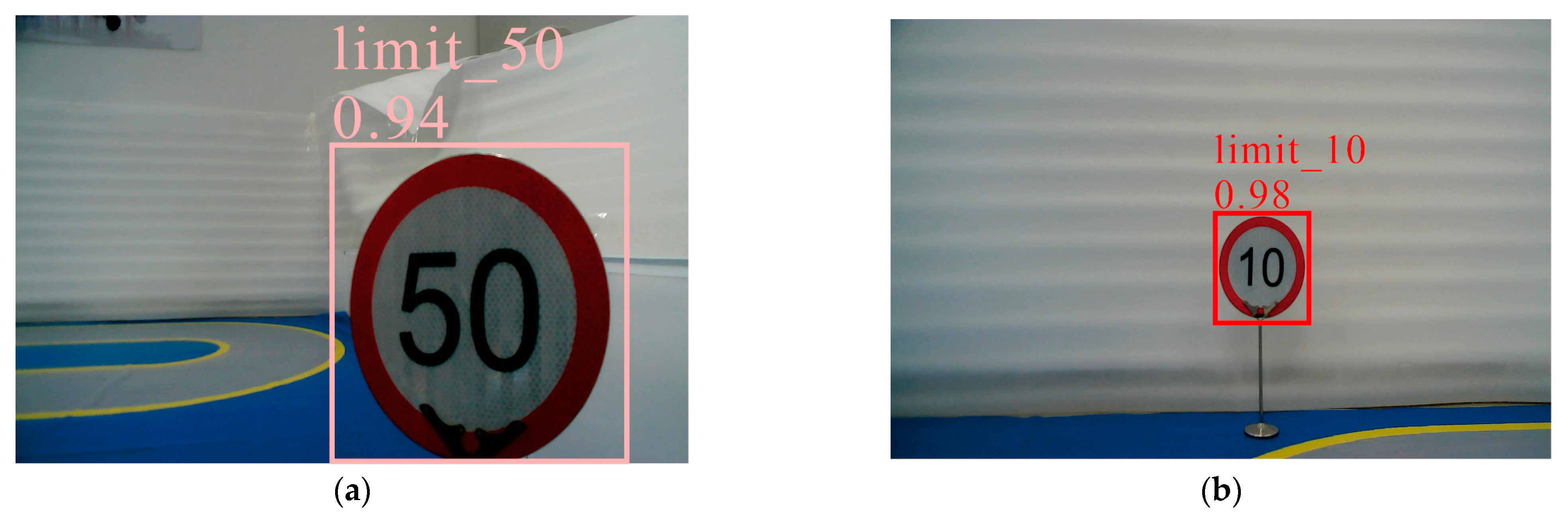
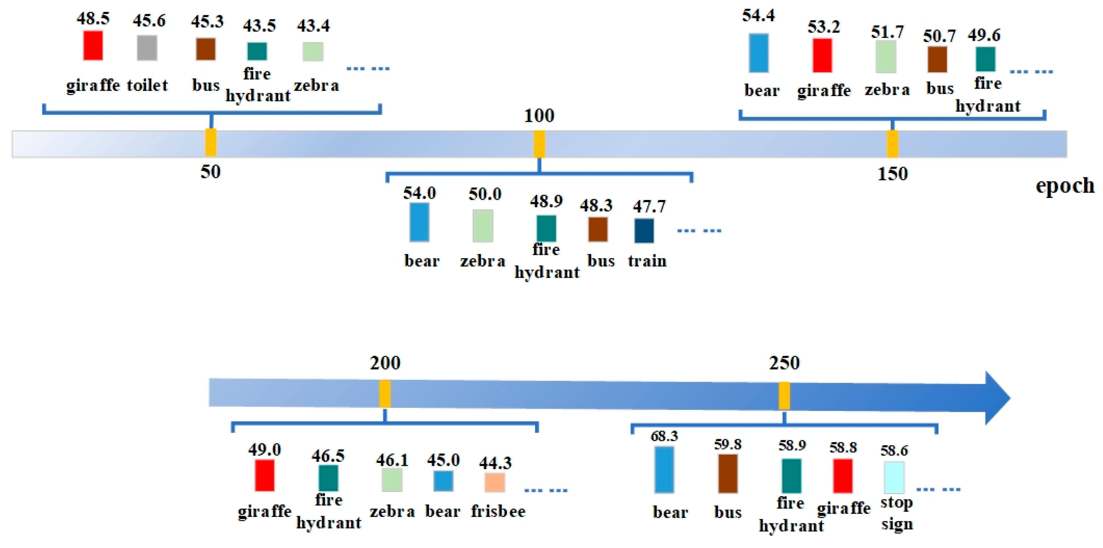
To provide an intuitive explanation of the above analysis, the model YOLOv3 was trained with the original COCO datasets. Figure 2 shows the evaluation results of these 5 nodes. The figure only shows the top 5 categories with the highest values. These 5 nodes are the 50th, 100th, 150th, 200th, and 250th epoch, respectively. From the figure, it can be seen that the evaluation results of the 200th epoch show a significant decrease compared to the results of the 100th and 150th epoch, and the training of the model is unstable. For the top five classes, there are differences in the evaluation results between the five epochs. The class giraffe is highest at epoch 50, but does not appear in the top five highest classes at epoch 100. The class bear does not appear in the 50th epoch, but appears in the next four extracts. The class bus does not appear in the top five highest epochs at the 200th epoch, but appears in the other four extractions. The four classes of toilet, train, frisbee, and stop sign appear only once in these five extractions.

The training preferences of the model will be different in different training stages. Therefore, it is not appropriate to reflect the training preference of the model only from the evaluation results of pre-training. In order to master the training preferences of different stages, the commonly used improvement method is to calculate the training preferences based on the evaluation results in real time, and then update the training dataset constantly. This is similar to difficult sample mining, which checks loss values or other indicators in real time to mine the information that the model needs to focus on learning. For the Copy-Paste augmentation algorithm, the main data amplification method is to insert the synthesized image in the training dataset, where the new training dataset is used to train the model. If real-time sampling is applied to the Copy-Paste augmentation algorithm, it means that the training dataset needs to be updated frequently, and it takes time to generate images and import a new training set. The frequent updating of the datasets results in a long training time. If the dataset is updated frequently, it does not give the model much additional class information to learn.

3.3. The Design of MSACP Algorithm

The model in the field of deep learning is usually regarded as a black box because the parameters of the model are uncertain during the training process. How does class imbalance affect model training? For supervised learning, the number of samples in the datasets and the model structure are known, which is a priori knowledge. The probability that the model predicts samples is the posterior probability. The class information such as speed limit signs, warning signs, and so on are in the TT100K dataset and are assumed to be independent of each other. The class information in the training dataset can be written as D = {(x₁,y₁), (x₂,y₂), (x₃,y₃), … …, (x_n,y_n)}, where x is the sample with class label y, and n is the number of classes. If the training dataset contains samples with {m₁, m₂, m₃, … …, m_m}, the probability that a predicted sample m belongs to class x_i can be written as Equation (1):

$$p(x_i|\mathrm{m})=\frac{p(\mathrm{m}|x_i)\times p(x_i)}{\sum _1^{\mathrm{n}}p({\mathrm{m}|x}_i)\times p(x_i)}$$

(1)

where $p(x_i|\mathrm{m})$ represents the probability that sample m is predicted by the model as class $x_i$. $p(x_i)$ is the prior probability of this class, which represents the proportion of the number of samples in the training dataset. $p(\mathrm{m}|x_i)$ is the conditional probability, representing the class $x_i$ of the training dataset. Equation (1) can be further simplified, as shown in Equation (2):

$$p(x_i|\mathrm{m})=\frac{p(\mathrm{m}|x_i)\times p(x_i)}{p(m)}$$

(2)

Among them, $p(x_i)$ is the proportion of the number of samples of class $x_i$ and the total number of samples in the training dataset. The conditional probability $p(\mathrm{m}|x_i)$ and prior probability $p(x_i)$ in the Bayesian model are related to the number of samples in the training dataset, so the class imbalance can affect the magnitude of these two probabilities. If ${\mathrm{c}}_{-}$ is used to represent the class with a large number of samples, and ${\mathrm{c}}_{+}$ is used to represent the class with a small number of samples, then the posterior probabilities of these two classes can be calculated by Bayes, as shown in Equations (3) and (4):

$$p({\mathrm{c}}_{-}|\mathrm{m})=\frac{p(\mathrm{m}|{\mathrm{c}}_{-})\times p({\mathrm{c}}_{-})}{p(m)}$$

(3)

$$p({\mathrm{c}}_{+}|\mathrm{m})=\frac{p(\mathrm{m}|{\mathrm{c}}_{+})\times p({\mathrm{c}}_{+})}{p(m)}$$

(4)

Because the number of samples for class ${\mathrm{c}}_{+}$ in the training dataset is small, the values of $p(\mathrm{m}|{\mathrm{c}}_{+})$ and $p({\mathrm{c}}_{+})$ are also small, which results in the posterior probability $p({\mathrm{c}}_{+}|\mathrm{m})$ becoming smaller. Because of the influence of class imbalance, the posterior probability of class $\mathrm{c}\_$ becomes larger, so the prediction result of the model will be biased to $\mathrm{c}\_$. To reduce the effect of class imbalance, the Copy-Paste enhancement algorithm is used to expand the class information with insufficient samples. This method is used to improve the prior probabilities of these classes and modify the prediction results of the model.

Due to its unique design, the model is easily able to grasp certain categories during training, which forms the training preferences of the model. Under the same dataset, the detection performance of the model is not positively correlated with the number of samples in the dataset. Although the number of samples in the training set is not very large for some categories, the model can accurately detect these categories. Therefore, simply using Copy-Paste enhancement algorithms to increase the sample size of a class lacks the support of principled approaches. After the analysis in Figure 2, the training preferences will change at different training nodes. These changes are used to update the category information of the training set, correct the training direction of the model, and further improve the detection performance of the model.

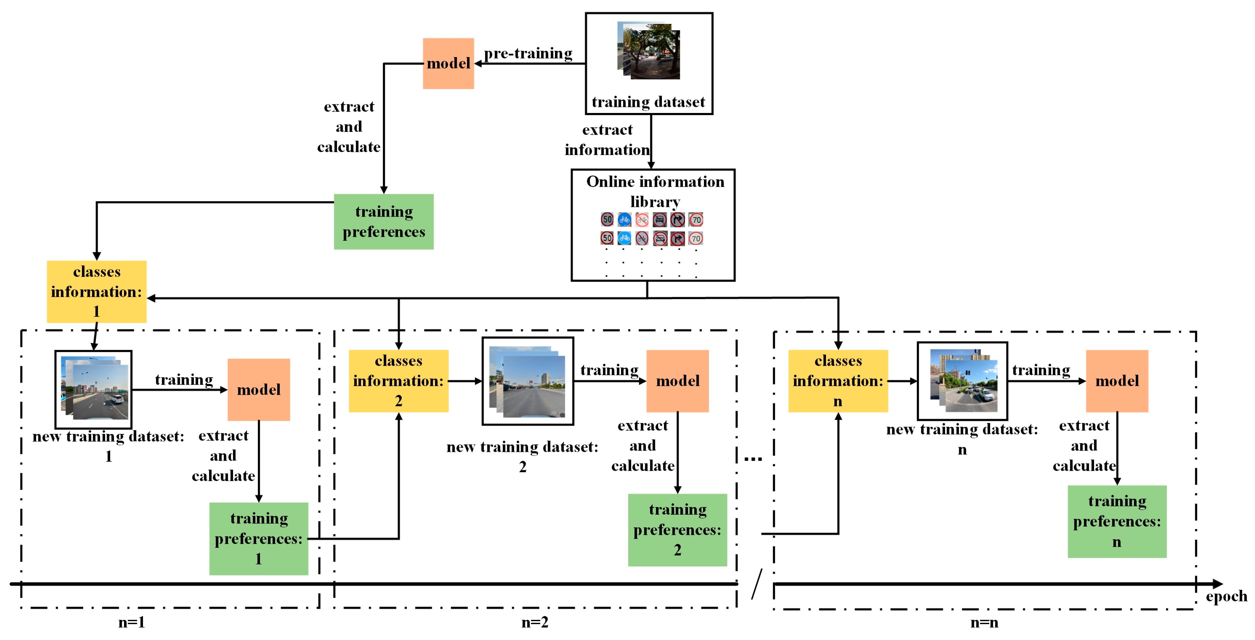
How to choose an appropriate time point to update the training dataset and open a new training stage? To ensure the simplicity and generality of MSACP algorithm, the training volume of the model is equally divided into stages. The hyper-parameter n is to represent the number of stages. Before starting the next training stage, MSACP algorithm adaptively adjusts the class information of the training dataset according to the training situation of the current stage. The key of MSACP algorithm is to amplify the appropriate class information according to the training preference of different stages. The computed expression for this training preference is given in Equation (5):

$$Class preference ({\mathrm{C}\mathrm{P}}_i)=p\left({AP}_i^{sf}-{AP}_i^{sl}\right)\times \left({AP}_i^{sl}-{mAP}^{sl}+T\right)$$

(5)

where ${\mathrm{C}\mathrm{P}}_i$ reflects the degree of preference of the model in the stage. ${AP}_i$ is the evaluation result for each class. i is id of the class. $sf$ is the evaluation result of the first epoch in this stage. Then $sl$ is the evaluation result of the last epoch in this stage. $p({AP}_i^{sf}-{AP}_i^{sl})$ serves as an enhancement coefficient to dynamically adjust the preference degree of classes, written as follows:

$$p\left({AP}_i^{sf}-{AP}_i^{sl}\right)=\left\{\begin{array}{c} 1, {AP}_i^{sf}-{AP}_i^{sl}<1 \\ {AP}_i^{sf}-{AP}_i^{sl}, {AP}_i^{sf}-{AP}_i^{sl}\ge 1\end{array}\right.$$

(6)

When ${AP}_i^{sf}-{AP}_i^{sl}$ is greater than 1, it means that in this stage, the detection effect of the model for the class is reduced and the training preference is enhanced. When ${AP}_i^{sf}-{AP}_i^{sl}$ is less than 1, it means that the detection effect of the model for the class remains stable or has been improved in this stage. The training preference is then kept constant. After obtaining the training preferences for the current stage, the MSACP algorithm calculates the number of samples that need to be expanded in this stage. According to the results, the appropriate amount of amplification is provided for the copy–move augmentation algorithm to adjust the class information in the training dataset. The expression is shown in Formula (7):

$$n_i^{\prime }={CP}_i\times n_i\times f\left({AP}_i^{sl}-{mAP}^{sl}+T\right)$$

(7)

$T$ is the regulation coefficient. The number of classes to be amplified is adjusted by the size of $T$. Finally, this result needs to be processed by the normalization, as shown in Formula (8):

$$Y_i=S_1+\frac{(S_2-S_1)}{[Max\left(n^{\prime }\right)-Min\left(n^{\prime }\right)]}\times [n_i^{\prime }-Min\left(n^{\prime }\right)]$$

(8)

(S₁, S₂) is the normalized range, $Y_i$ is the final output result of the class. $n^{\prime } \mathrm{i}\mathrm{s} \mathrm{t}\mathrm{h}\mathrm{e} \mathrm{s}\mathrm{e}\mathrm{t} \mathrm{o}\mathrm{f} n_i^{\prime }$.

4. Results

In this part, the effectiveness and generality of the MSACP algorithm are verified by experiments from multiple perspectives. First, the basic environment and dataset used in the experiment are introduced in Section 4.1. Then, the validity and generality of the MSACP algorithm are verified with the TT100K dataset in Section 4.2 and Section 4.3. Finally, the results and phenomena during the experiments are analyzed in Section 4.4.

4.1. Experimental Environments

All experiments were performed using Ubuntu 20.04 (Canonical, Cape Town, South Africa) and four RTX-3090 GPUs (NVIDIA, Santa Clara, CA, USA). In terms of datasets, the MSACP algorithm is validated using the TT100K [33] dataset. Only classes with a sample size greater than 100 are used in the experiment. There are 42 classes. The number of classes in TT100K is randomly divided into training datasets, validation datasets, and test datasets at a ratio of 7:2:1. The MSACP algorithm operates on the training dataset.

4.2. Performance Testing of MSACP in Different Models

In this section, the effectiveness of MSACP is tested on Grid RCNN [15], ATSS [16], and AutoAssign [34]. It is necessary to examine the effectiveness of the MSACP algorithm by using models with different structures. The RCNN and ATSS models belong to the two-stage range. The AutoAssign model belongs to the one-stage range. The epoch of all three models is 12. Two sets of experiments were set up for comparative analysis. The first comparison method was the origin, where the model was trained on the original dataset. The other comparison method was the CPA algorithm, which is for special cases when n = 1. The model was trained with the training dataset optimized by the CPA algorithm. It can be seen from the three tables that the CPA algorithm is obviously better than the original TT100K dataset for training. The MSACP algorithm makes up for the deficiency of the CPA algorithm in expanding sample information. The algorithm can continuously modify the expanded sample size according to the training preferences of different stages.

There are two key steps to complete before formal training. First, an online class database needs to be created to simplify the process of updating the training dataset. The class information in the training dataset is cut according to the corresponding label files, and then the information is classified by category. In addition, this class information is processed by a variety of data augmentation, such as color shifts, flips, random occlusion, etc. The class information in the online library is extracted when the training dataset needs to be updated. The second step is to pre-train the model with the original datasets. The evaluation results of pre-training are extracted and the training preferences of the model in the pre-training are calculated. The calculated results are used to optimize the class information in the training dataset. This training dataset will be used for the first stage of formal model training. When n is set to two, it means that the overall training amount is divided into two training stages by the MSACP algorithm. Before starting the next stage, training preferences are calculated based on the evaluation results of the current stage. Based on this result, the MSACP algorithm can amplify the appropriate amount of information for each class, which can reduce the phenomenon of overfitting or underfitting.

As shown in

Table 1. The training results are compared by the Grid RCNN model (epoch = 12).

Method	AP (%)	AP50 (%)	AP75 (%)	APs (%)	APm (%)	APl (%)
origin	43.4	53.4	51.0	8.7	58.5	81.7
CPA	49.7	62.3	58.9	10.7	66.7	84.7
n = 2	50.0	62.6	58.8	9.6	66.7	84.7
n = 3	50.7	63.4	59.5	10.5	68.4	85.7
n = 4	50.9	63.5	59.5	11.1	68.6	86.7

, the CPA algorithm has an obvious improvement effect on Grid RCNN because the class imbalance of the TT100K dataset is serious. In the three optimization experiments of the MSACP algorithm, the overall improvement effect is best when n is equal to four. The AP is increased by 1.2% compared with the CPA algorithm. Since the epoch of Grid RCNN is 12, the model will calculate the training preferences based on the evaluation results when trained to epoch = 3, epoch = 6, and epoch = 9, respectively. The MSACP algorithm updates the training set based on the generated results. After the new training set is imported, the model begins the next stage of training. When n = 2 and n = 3, the corresponding AP increased by 0.3% and 1% compared to the CPA algorithm, respectively.

The MSACP algorithm is embedded into the ATSS, and the results of the experiment are shown in

Table 2. The training results are compared by the ATSS model (epoch = 12).

Method	AP (%)	AP50 (%)	AP75 (%)	APs (%)	APm (%)	APl (%)
origin	39.3	51.1	45.7	15.5	48.8	69.4
CPA	48.4	62.1	56.4	13.7	61.2	84.2
n = 2	48.8	62.4	56.9	13.6	61.5	85.5
n = 3	49.0	62.7	57.0	13.5	61.6	85.5
n = 4	48.7	62.4	56.6	13.7	61.3	85.5

. In the three optimization experiments, the overall improvement effect is best when n is set to three. The AP is increased by 1.2% compared with the CPA algorithm. When n = 2 and n = 4, the AP increases by 0.4% and 0.3%, respectively, compared with the CPA algorithm. For

Table 3. The training results are compared by the AutoAssign model (epoch = 12).

Method	AP (%)	AP50 (%)	AP75 (%)	APs (%)	APm (%)	APl (%)
origin	48.0	66.2	55.5	25.8	58	75.6
CPA	49.9	66.5	58	21.4	60.3	80.7
n = 2	53.4	71.6	61.9	22.9	64.8	82.1
n = 3	52.7	70.9	60.7	23.6	63.8	82.5
n = 4	52.5	70.5	61.3	23.5	63.7	80.8

, the MSACP algorithm was embedded into the AutoAssign model. In three optimization experiments, the overall improvement effect is best when n is set to two. The AP is improved by 3.5% compared with the CPA algorithm. When n = 3 and n = 4, the AP is increased by 2.8% and 2.6% compared with the CPA algorithm, respectively. The MSACP algorithm provides phased optimization for the training dataset according to the training information, which makes the information distribution actively adapt to different stages of model training.

4.3. Performance Detection of MSACP under Different Training Amounts

The MSACP algorithm divides the total training amount into multiple stages on average. Before starting the next stage of training, the class information of the training dataset will be adjusted adaptively according to the training situation of the current stage. The amount of training in each stage is related to the amount of the hyper-parameters, epoch and n. In Section 3.2, the epochs of the models were all 12. It is necessary to use the MSACP algorithm to examine models with a different epoch.

In this section, three models with more epochs are selected, including SSD512 [35], NAS FGN [36], and YOLOv3 [17]. The SSD512 and YOLOv3 models belong to the one-stage range. The NAS FGN model is a classic feature pyramid network. Their experimental results are listed in

Table 4. The training results are compared by the SSD512 model (epoch = 24).

Method	AP (%)	AP50 (%)	AP75 (%)	APs (%)	APm (%)	APl (%)
origin	50.4	74.9	56.6	22.9	61.9	83.1
CPA	52.4	75.9	59.3	22.5	64.2	84.1
n = 2	52.9	76.4	59.6	21.7	64.6	84.9
n = 3	52.6	76.7	58.5	22.3	64.0	84.7
n = 4	52.8	76.2	59.1	23.3	64.2	85.5

,

Table 5. The training results are compared by the NAS FGN model (epoch = 50).

Method	AP (%)	AP50 (%)	AP75 (%)	APs (%)	APm (%)	APl (%)
origin	25.9	41.4	27.4	15.7	32.9	51.2
CPA	39.6	56.3	43.5	16.2	46.8	81.6
n = 2	40.0	56.8	44.4	16.0	47.5	81.0
n = 3	40.1	56.8	44.6	16.8	47.7	81.2
n = 4	40.8	57.5	45.4	16.4	49.0	82.4

and

Table 6. The training results are compared by the YOLOv3 model (epoch = 273).

Method	AP (%)	AP50 (%)	AP75 (%)	APs (%)	APm (%)	APl (%)
origin	50.3	76.8	58.3	37.8	59.3	62.1
CPA	57.9	84.9	66.3	37.2	68.3	76.7
n = 2	58.3	85.6	67.7	38.6	68.8	76.6
n = 3	58.4	85.5	68.1	39.7	68.9	75.2
n = 4	58.6	85.8	67.4	38.0	69.4	77.4
n = 5	59.0	86.2	68.2	39.1	69.6	77.3

, respectively. For Table 4, the MSACP algorithm is tested with the model SSD512. The epoch of this model is 24. In these three experiments, the overall improvement effect of model SSD512 is the best when n = 2. The AP reaches 52.9%, which is improved by 0.5% over the CPA algorithm. When n = 3 and n = 4, the corresponding AP increases by 0.2% and 0.4% compared to the CPA algorithm, respectively. MSACP adaptively adjusts the class information of the training dataset according to the training condition of the model SSD512 to improve the training quality.

The effect of the MSACP algorithm was tested with the NAS FGN model. The results are shown in Table 5. When n = 4, the overall effect of model NAS FGN is the best, reaching 40.8%, which is improved by 1.2% compared with CPA. When n = 2 and n = 3, the corresponding AP of our proposed method increases by 0.4% and 0.5% compared to the CPA, respectively. MSACP adaptively adjusts the class information of the training dataset according to the training condition of the NAS FGN, which forces the model to pay more attention to the poorly learned classes in different training stages.

According to Table 6, when n = 5, the AP of model YOLOv3 reached 59.0%, which is increased by 1.1% compared with CPA. When n = 2, n = 3, and n = 4, the corresponding AP increases by 0.4%, 0.5%, and 0.7% compared to the CPA algorithm, respectively. From these three experiments, MSACP can still improve the model with a large number of epochs. Each model will show different tendencies to different classes in training because of its own unique structure. MSACP can provide dynamic information compensations for model training according to this tendency, which provides a reasonable enhancement amplitude for the Copy-Paste augmentation algorithm. Therefore, in the process of model training, each class can receive reasonable attention and learning, which avoids the phenomenon of overfitting or underfitting caused by unreasonable information expansion, and improves the robustness of the model.

4.4. Discussions

To analyze the experimental phenomenon in detail, the experimental results of AutoAssign are visually analyzed. The number of expanded samples after CPA optimization and the evaluation results of each class are shown in Figure 3. The horizontal coordinate is the class of the TT100K dataset. The hyper-parameters e and T in the CPA algorithm are set to 2.5 and 0.05, respectively. It can be seen from Figure 3 that 15 classes in the TT100K dataset are not amplified by the CPA algorithm. This is due to the fact that each of these classes has a high AP or contains a very large sample size. Other classes are amplified because they contain less information in the training dataset and their APs are not ideal.

Two sets of experimental data for the model AutoAssign are visualized, including the experiments with n = 2 and n = 3 in Table 3. The results of updating the model AutoAssign when n = 2 is shown in Figure 4. The blue bar is the number of samples in the original training dataset. The orange bar is the number of samples amplified by the MSACP algorithm. The height of the two columns is the number of samples in the updated training dataset. The broken line in the figure is the evaluation results when the model AutoAssign is trained to epoch = 6. The training preference is calculated by the MSACP algorithm to amplify the appropriate class information for each class according to the current training situation. In this data update, there are 11 categories that have not been amplified in the TT100K dataset.

Figure 5 and Figure 6 show the data updates of the AutoAssign model when n = 3. For Figure 5, this is the evaluation when the model AutoAssign is trained to epoch = 4. There are 11 classes in the dataset that have not been expanded by MSACP. i4, i5, il100, il60, ip, p23, p27, pl100, and pr40 have not been amplified because these classes have higher AP.

Figure 6 shows the second data update of the AutoAssign model when n = 3. The result of AutoAssign is trained to epoch = 8. There are 14 classes in the figure that have not been expanded by MSACP. i4, i5, il100, il60, p26, p5, pg, pl100, p11, pl120, pl40, and pr4 do not have amplification information because these classes have higher APs. Compared with the first data update with n = 3, three more classes of information were amplified in this update, namely, p26, p5, and pl40. For example, the model does not pay much attention to category pl40 in early training, which leads to poor model detection of this class. The MSACP algorithm adjusts the model’s attention to this class with information compensation. In the second data update, class pl40 does not need compensation for the information by MSACP because it has a higher AP. The class information is updated according to the different stages of training.

According to the data visualization of the MSACP experiment, the expanded sample quantity of each category is different in the three updates. By dividing the training amount into multiple stages, MSACP dynamically adjusts the class information of the training dataset and modifies the learning direction of the model at intervals according to the learning situation. This kind of dynamic adjustment at intervals not only reduces the computing power requirement of training, but also alleviates the class imbalance.

Six models are used to verify the effectiveness of the MSACP algorithm. There are three models that achieve better results when n = 4, namely, Grid RCNN, NAS FGN, and YOLOv3. The other three models achieve better results when n = 2 or n = 3. From the experimental results, it can be seen that more training stages do not necessarily make the model obtain a better improvement effect. When n is greater than four, these models are likely to have better results. The larger the n, the more time it takes to update the training dataset, which leads to a longer training time. When n = 1, the training of the model has only one stage and the training set is not updated. The entire training of the AutoAssign model takes approximately 270 min. When n is greater than one, the training dataset is updated by MSACP. For AutoAssign, it takes about 30 min to complete an update of the training dataset and start the next stage of training. When n = 4, the total running time of MSACP is about 120 min, as shown in

Table 7. The time of AutoAssign model to update the training dataset by MSACP.

n	Time (min)	$\mathbf{A}\mathbf{P}$ (%)
1	270	48.0
2	300	53.4
3	330	52.7
4	370	52.5

. Although better detection performance may occur if the hyper-parameter n is set larger, there is not much room for improvement in the model. Under the comprehensive consideration of training time and performance improvement, the experiment only set four groups to test the impact of n on the MSACP algorithm.

5. Embedded Application of MSACP Algorithm

Many deep learning algorithms have been applied in real life, but there are also many challenges in the practical application. How to improve the performance of the embedded platform under the limited computing power is one of the main challenges. Therefore, MSACP is applied to the autonomous driving scenario to test the effect of the algorithm in practical applications. The scenario is shown in Figure 7. It can be seen that the autonomous driving scenario has multiple speed limit signs and a traffic light. The embedded platform is in the red box, which is equipped with a CPU of 4-core ARM Cortex-57 series (ARM, Cambridge, UK) and a GPU of 128-core Maxwell architecture (NVIDIA, Santa Clara, CA, USA). The computing power is not less than 472 GFLOPs. In addition, the platform is equipped with a human–computer interaction interface, which can output the road condition information and detect the corresponding object information in real time.

The model YOLOv3-tiny is selected for traffic sign detection in the embedded platform, which is a simplified version of YOLOv3. Yolov3-tiny mainly removes some feature layers based on YOLOv3, and at the same time changes the three independent prediction branches into two. Therefore, YOLOv3-tiny has a faster inference speed and is widely used in practical projects. The dataset used in this experiment contains 12 classes, some of which are difficult to collect in real life. There is still an imbalance of categories in the dataset. The class of people and car in the dataset has the largest number of samples, while the class with the smallest number of samples is yellow light. Because of the cost and time of production, MSACP is used to optimize the dataset, which is embedded into the YOLOv3-tiny model. The optimal weight file is obtained after the training is completed and deployed to the embedded platform for object detection. A comparative test is performed before importing the embedded platform, as shown in

Table 8. The comparison of class performances based on the YOLOv3-tiny model.

Class	YOLOv3-Tiny (%)	YOLOv3-Tiny + MSACP(%)
green_light	78.8	76.8 (−2.0)
yellow_light	97.0	98.4 (+1.4)
red_light	68.8	70.3 (+1.5)
turn_right	85.2	83.4 (−1.8)
turn_left	77.4	82.3 (+4.9)
limit_10	72.0	99.5 (+27.5)
limit_50	85.6	91.3 (+5.7)
limit_60	95.6	95.6 (+0.0)
limit_110	94.5	96.9 (+2.4)
person	99.3	99.4 (+0.1)
car	99.5	99.5 (+0.0)
stop	99.5	99.5 (+0.0)
Average	87.8	91.1 (+3.3)

. The metric used in the table is AP₅₀. The YOLOv3-tiny model with the MSACP algorithm is improved by 3.3% compared to the original model. Some classes have significant improvements, such as limit_10 and limit_50.

In addition, a more intuitive experiment was performed. Three images with traffic signs on which the model had not been trained were randomly selected for testing. The results are shown in Figure 8 and Figure 9. Figure 8 shows the detection results of YOLOv3-tiny. Figure 9 shows the detection results of YOLOv3-tiny + MSACP. From the visual results, the YOLOv3-tiny model with MSACP has higher confidence in detecting traffic signs. More importantly, the inference time is the same for both comparisons.

6. Conclusions

In this paper, we propose MSACP, a multi-stage adaptive Copy-Paste augmentation method based on model training preference. MSACP introduces a multi-stage adjustment mechanism to provide dynamic information compensations for the training of the model. Under the premise of alleviating class imbalance, the over-fitting or under-fitting phenomenon generated in the training of the model is avoided as much as possible. Although the MSACP algorithm is effective according to the experimental results, it takes a long time to update the training dataset. When the MSACP algorithm processes complex data such as 3D images, the operation among objects easily destroys key information in the image, and even generates data that are not conducive to model training. In future work, this is one of the difficulties that we will focus on overcoming. In addition, we hope that the multi-stage adjustment mechanism in the MSACP algorithm can further be applied to different data enhancement strategies so that data augmentation can play an effective role in model training.

References

1. Oksuz, K.; Cam, B.C.; Kalkan, S.; Akbas, E. Imbalance problems in object detection: A review. IEEE Trans. Pattern Anal. Mach. Intell. 2020, 43, 3388–3415. [Google Scholar] [CrossRef] [PubMed]
2. Zhang, Y.; Kang, B.; Hooi, B.; Yan, S.; Feng, J. Deep Long-Tailed Learning: A Survey. IEEE Trans. Pattern Anal. Mach. Intell. 2023, 45, 10795–10816. [Google Scholar] [CrossRef] [PubMed]
3. Feng, C.; Zhong, Y.; Huang, W. Exploring classification equilibrium in long-tailed object detection. In Proceedings of the IEEE/CVF International Conference on Computer Vision, Montreal, BC, Canada, 11–17 October 2021; pp. 3417–3426. [Google Scholar]
4. Wang, Y.; Gan, W.; Yang, J.; Wu, W.; Yan, J. Dynamic curriculum learning for imbalanced data classification. In Proceedings of the IEEE/CVF International Conference on Computer Vision, Seoul, Republic of Korea, 27 October–2 November 2019; pp. 5017–5026. [Google Scholar]
5. Shrivastava, A.; Gupta, A.; Girshick, R. Training region-based object detectors with online hard example mining. In Proceedings of the IEEE Conference on Computer Vision and Pattern Recognition, Las Vegas, NV, USA, 27–30 June 2016; pp. 761–769. [Google Scholar]
6. Shorten, C.; Khoshgoftaar, T.M. A survey on image data augmentation for deep learning. J. Big Data 2019, 6, 1–48. [Google Scholar] [CrossRef]
7. Chen, P.; Liu, S.; Zhao, H.; Jia, J. Gridmask data augmentation. arXiv 2020, arXiv:2001.04086. [Google Scholar]
8. Bochkovskiy, A.; Wang, C.Y.; Liao, H.Y.M. Yolov4: Optimal speed and accuracy of object detection. arXiv 2020, arXiv:2004.10934. [Google Scholar]
9. Huang, S.W.; Lin, C.T.; Chen, S.P.; Wu, Y.Y.; Hsu, P.H.; Lai, S.H. Auggan: Cross domain adaptation with gan-based data augmentation. In Proceedings of the European Conference on Computer Vision (ECCV), Munich, Germany, 8–14 September 2018; pp. 718–731. [Google Scholar]
10. Ghiasi, G.; Cui, Y.; Srinivas, A.; Qian, R.; Lin, T.-Y.; Cubuk, E.D.; Le, Q.V.; Zoph, B. Simple copy-paste is a strong data augmentation method for instance segmentation. In Proceedings of the IEEE/CVF Conference on Computer Vision and Pattern Recognition, Nashville, TN, USA, 20–25 June 2021; pp. 2918–2928. [Google Scholar]
11. Dwibedi, D.; Misra, I.; Hebert, M. Cut, paste and learn: Surprisingly easy synthesis for instance detection. In Proceedings of the IEEE International Conference on Computer Vision, Venice, Italy, 22–29 October 2017; pp. 1301–1310. [Google Scholar]
12. Cubuk, E.D.; Zoph, B.; Mane, D.; Vasudevan, V.; Le, Q.V. Autoaugment: Learning augmentation strategies from data. In Proceedings of the IEEE/CVF Conference on Computer Vision and Pattern Recognition, Long Beach, CA, USA, 15–20 June 2019; pp. 113–123. [Google Scholar]
13. Lim, S.; Kim, I.; Kim, T.; Kim, C.; Kim, S. Fast AutoAugment. In Proceedings of the 33rd International Conference on Neural Information Processing Systems, Vancouver, BC, Canada, 8–14 December 2019; pp. 6665–6675. [Google Scholar]
14. Yu, X.; Li, F.; Bai, P.; Liu, Y.; Chen, Y. Copy-paste with self-adaptation: A self-adaptive adjustment method based on copy-paste augmentation. IET Comput. Vis. 2023. [Google Scholar] [CrossRef]
15. Lu, X.; Li, B.; Yue, Y.; Li, Q.; Yan, J. Grid r-cnn. In Proceedings of the IEEE/CVF Conference on Computer Vision and Pattern Recognition, Long Beach, CA, USA, 15–20 June 2019; pp. 7363–7372. [Google Scholar]
16. Zhang, S.; Chi, C.; Yao, Y.; Lei, Z.; Li, S.Z. Bridging the gap between anchor-based and anchor-free detection via adaptive training sample selection. In Proceedings of the IEEE/CVF Conference on Computer Vision and Pattern Recognition, Seattle, WA, USA, 13–19 June 2020; pp. 9759–9768. [Google Scholar]
17. Redmon, J.; Farhadi, A. Yolov3: An incremental improvement. arXiv 2018, arXiv:1804.02767. [Google Scholar]
18. Lin, T.Y.; Goyal, P.; Girshick, R.; He, K.; Dollár, P. Focal loss for dense object detection. In Proceedings of the IEEE International Conference on Computer Vision, Venice, Italy, 22–29 October 2017; pp. 2980–2988. [Google Scholar]
19. Wang, T.; Zhu, Y.; Zhao, C.; Zeng, W.; Wang, J.; Tang, M. Adaptive class suppression loss for long-tail object detection. In Proceedings of the IEEE/CVF International Conference on Computer Vision, Montreal, BC, Canada, 11–17 October 2021; pp. 3103–3112. [Google Scholar]
20. Tan, J.; Wang, C.; Li, B.; Li, Q.; Ouyang, W.; Yin, C.; Yan, J. Equalization loss for long-tailed object recognition. In Proceedings of the IEEE/CVF Conference on Computer Vision and Pattern Recognition, Seattle, WA, USA, 13–19 June 2020; pp. 11662–11671. [Google Scholar]
21. Menon, A.K.; Jayasumana, S.; Rawat, A.S.; Jain, H.; Veit, A.; Kumar, S. Long-tail learning via logit adjustment. In Proceedings of the International Conference on Learning Representations, Addis Ababa, Ethiopia, 26–30 April 2020. [Google Scholar]
22. Li, T.; Cao, P.; Yuan, Y.; Fan, L.; Yang, Y.; Feris, R.S.; Indyk, P.; Katabi, D. Targeted supervised contrastive learning for long-tailed recognition. In Proceedings of the IEEE/CVF Conference on Computer Vision and Pattern Recognition, New Orleans, LA, USA, 19–20 June 2022; pp. 6918–6928. [Google Scholar]
23. Cui, Y.; Jia, M.; Lin, T.Y.; Song, Y.; Belongie, S. Class-balanced loss based on effective number of samples. In Proceedings of the IEEE/CVF Conference on Computer Vision and Pattern Recognition, Long Beach, CA, USA, 15–20 June 2019; pp. 9268–9277. [Google Scholar]
24. Yun, S.; Han, D.; Oh, S.J.; Chun, S.; Choe, J.; Yoo, Y. Cutmix: Regularization strategy to train strong classifiers with localizable features. In Proceedings of the IEEE/CVF Conference on Computer Vision and Pattern Recognition, Long Beach, CA, USA, 15–20 June 2019; pp. 6023–6032. [Google Scholar]
25. Kisantal, M.; Wojna, Z.; Murawski, J.; Naruniec, J.; Cho, K. Augmentation for small object detection. CS IT Conf. Proc. 2019, 9, 119–133. [Google Scholar]
26. Dvornik, N.; Mairal, J.; Schmid, C. Modeling visual context is key to augmenting object detection datasets. In Proceedings of the European Conference on Computer Vision (ECCV), Munich, Germany, 8–14 September 2018; pp. 364–380. [Google Scholar]
27. Li, C.L.; Sohn, K.; Yoon, J.; Pfister, T. Cutpaste: Self-supervised learning for anomaly detection and localization. In Proceedings of the IEEE/CVF Conference on Computer Vision and Pattern Recognition, Nashville, TN, USA, 20–25 June 2021; pp. 9664–9674. [Google Scholar]
28. Georgakis, G.; Mousavian, A.; Berg, A.C.; Kosecka, J. Synthesizing training data for object detection in indoor scenes. arXiv 2017, arXiv:1702.07836. [Google Scholar]
29. Yun, W.H.; Kim, T.; Lee, J.; Kim, J.; Kim, J. Cut-and-paste dataset generation for balancing domain gaps in object instance detection. IEEE Access 2021, 9, 14319–14329. [Google Scholar] [CrossRef]
30. Zhang, W.; Wang, Z.; Loy, C.C. Exploring Data Augmentation for Multi-Modality 3D Object Detection. In Proceedings of the International Conference on Learning Representations 2023 Workshop on Scene Representations for Autonomous Driving, Kigali, Rwanda, 1–5 May 2023. [Google Scholar]
31. Cubuk, E.D.; Zoph, B.; Shlens, J.; Le, Q.V. Randaugment: Practical automated data augmentation with a reduced search space. In Proceedings of the IEEE/CVF Conference on Computer Vision and Pattern Recognition Workshops, Seattle, WA, USA, 14–19 June 2020; pp. 702–703. [Google Scholar]
32. Lin, S.; Yu, T.; Feng, R.; Li, X.; Yu, X.; Xiao, L.; Chen, Z. Local patch autoaugment with multi-agent collaboration. arXiv 2021, arXiv:2103.11099. [Google Scholar] [CrossRef]
33. Zhu, Z.; Liang, D.; Zhang, S.; Huang, X.; Li, B.; Hu, S. Traffic-sign detection and classification in the wild. In Proceedings of the IEEE Conference on Computer Vision and Pattern Recognition, Las Vegas, NV, USA, 27–30 June 2016; pp. 2110–2118. [Google Scholar]
34. Zhu, B.; Wang, J.; Jiang, Z.; Zong, F.; Liu, S.; Li, Z.; Sun, J. Autoassign: Differentiable label assignment for dense object detection. arXiv 2020, arXiv:2007.03496. [Google Scholar]
35. Liu, W.; Anguelov, D.; Erhan, D.; Szegedy, C.; Reed, S.; Fu, C.Y.; Berg, A.C. Ssd: Single shot multibox detector. In Proceedings of the Computer Vision–ECCV 2016: 14th European Conference, Amsterdam, The Netherlands, 11–14 October 2016; Proceedings, Part I 14. Springer International Publishing: Berlin/Heidelberg, Germany, 2016; pp. 21–37. [Google Scholar]
36. Ghiasi, G.; Lin, T.Y.; Le, Q.V. Nas-fpn: Learning scalable feature pyramid architecture for object detection. In Proceedings of the IEEE/CVF Conference on Computer Vision and Pattern Recognition, Long Beach, CA, USA, 15–20 June 2019; pp. 7036–7045. [Google Scholar]
Figure 1. The training process of MSACP algorithm embedded in the model is shown.
Electronics 12 03695 g001
Figure 2. The evaluation results of model YOLOv3 in different stages on COCO dataset.
Electronics 12 03695 g002
Figure 3. Updated training dataset by the CPA and evaluation results of AutoAssign.
Electronics 12 03695 g003
Figure 4. Updated training dataset by MSACP and corresponding evaluation results at n = 2.
Electronics 12 03695 g004
Figure 5. The first updated training dataset by MSACP and corresponding evaluation results of AutoAssign at n = 3.
Electronics 12 03695 g005
Figure 6. The second updated training dataset by MSACP and corresponding evaluation results of AutoAssign at n = 3.
Electronics 12 03695 g006
Figure 7. The scene of simulated autonomous driving.
Electronics 12 03695 g007
Figure 8. The detection effect of YOLOv3-tiny: (a) The class of speed limit 50 km/h; (b) The class of speed limit 10 km/h.
Electronics 12 03695 g008
Figure 9. The detection effect of YOLOv3-tiny + MSACP: (a) The class of speed limit 50 km/h; (b) The class of speed limit 10 km/h.
Electronics 12 03695 g009