5G and Beyond: Channel Classification Enhancement Using VIF-Driven Preprocessing and Machine Learning

Abstract

The classification of wireless communication channel scenarios is vital for modern wireless technologies. Efficient data preprocessing for identification, especially starting from 5G and beyond, where multiple scenario transitions occur, is crucial. Machine Learning (ML) is employed for scenario identification. Moreover, accurate ML classification is required to enhance the decision-making process in each communication layer. The proposed model in this study utilizes an enhanced preprocessing phase. The proposed model proves that adding the variance inflation factor (VIF) elimination layer has a significant effect in eliminating the residual noise after regularization. By evaluating the VIF, the high multi-collinear features are removed after adding a regularization penalty. Consequently, the total explained variance (TEV) was enhanced by 5% and reached 76%. Thus, the classification accuracy of the identification processes of different rural and urban scenarios was increased by 3%, on average, compared with previous work for each algorithm: Random Forest (RF), K-Nearest Neighbor (KNN), Support Vector Machine (SVM), and Gaussian Mixture model (GMM).

1. Introduction

Nowadays, artificial intelligence (AI) plays an important role in modern wireless communication technology, in addition to industries, like science, medicine, and manufacturing [1]. Due to the growing number of smart devices, the rise of the Internet of Things (IoT), and the need for more worldwide connectivity, connecting isolated and rural places is essential [2]. Adding AI to modern wireless systems helps in processing large amounts of data received from devices, like smartphones, laptops, tablets, and sensors, efficiently. ML is a subset of AI that uses massive volumes of data to train algorithms and enhance their comprehension of processed information [3]. The trained ML algorithms can make predictions and decisions based on new data, optimizing the automated networks in 5G and beyond, to meet Quality of Service (QoS) requirements. The goal of 5G and beyond is to provide diverse services and seamless global network coverage. The integration of satellite and terrestrial networks is being explored to offer worldwide broadband connectivity [4], attracting interest from academia and the business sector.

Wireless communication systems have three layers: the physical-, middle-, and end-user layers. To improve the QoS, system security, privacy, latency, power allocation and control, and channel capacity, AI techniques are applied at every layer. In the physical layer, ML plays a vital role in tasks, like channel encoding, decoding, and estimation. Scenario classification, an ML application, involves estimating the channel environment for data transmission. Scenarios can include rural, suburban, urban, indoor hotspots, and satellites. Urban macro cells (UMa) are deployed in cities, while rural macro cells (RMa) are used in less populated and scattered rural areas [5]. Users often encounter various scenarios, like deserts, mountains, stations, and obstacles, especially during high-speed transportation. These scenarios strain communication systems, necessitating an accurate definition of wireless channel scenarios to meet user QoS requirements.

In a wireless communication system, inaccurate identification of the channel mode, where prior knowledge of the possible propagation models such as traditional statistical models Okumura and Hata is assumed, can lead to inaccuracies in data interpretation and system performance. Minimizing complexity and runtime while precisely identifying the channel model scenario are crucial steps for reliable communication systems. Power efficiency, beam management, maintenance, bandwidth allocation, network setup, operation, throughput, QoS prediction, and coverage performance are all addressed by AI-based solutions.

Deep learning (DL) methods are commonly used but require more computational time. DL has been used in previous studies to differentiate between line-of-sight (LoS) and non-line-of-sight (NLoS) scenarios in urban settings utilizing elevation and azimuth angles [6]. Convolutional networks have achieved accurate classification in fingerprint feature extraction and classification tasks [7]. The effectiveness of supervised classification algorithms and unsupervised learning clustering algorithms for scenario identification has also been demonstrated [8,9,10].

Recently, in [8], it was shown that the utilization of the least absolute shrinkage and selection operator (LASSO) could optimize timing and performance for wireless communication typical terrestrial scenario classification rather than ElasticNet. Therefore, the previous consecutive works [8,9] demonstrated how regularizing the feature selection process could improve the classification performance of [10] and reduce the computational complexity of ML algorithms while preserving strong generalization capabilities. Nevertheless, it is still necessary to reduce the computational burden of the preprocessing step and the algorithm’s classification time in order to swiftly identify scenarios during transitions between multiple scenarios.

The main contributions of this work are:

• Lowering the model responsiveness and latency for each regularization technique instruction used in the prior model’s preprocessing workflow [8,9]. In this work, the regularization procedures are enhanced by adding another filtration layer based on VIF. This layer could remove multicollinearity existing in the elevation spread angle of arrival (esA). This process could increase the performance and time efficiency for both preprocessing and classification tasks.
• Utilization time for kernel principal component analysis (k-PCA) is decreased, as it reduces the dimension of the features from three to two instead of from four to two like the previous work [8]. Moreover, at the ML layer, the RF algorithm was evaluated and compared with KNN, SVM, and GMM. It achieved 100% accuracy in testing data.

The remaining sections of this paper are structured in the following manner. In Section 2, details regarding the dataset, as well as the procedures for preprocessing and processing, are presented. Section 3 presents the outcomes and discussions of the preprocessing and classification phase. Finally, Section 4 focuses on the main conclusions derived from the study.

2. Wireless Communication Model Dataset

This section provides a comprehensive discussion of the dataset utilized in this study. The features describing each wireless communication scenario, including delay spread ($D_{\sigma }$), Path Loss ($P_L$), K-Factor ($K_F$), elevation spread angle of arrival (${\sigma }_{EoA}$), elevation spread angle of departure (${\sigma }_{EoD}$), azimuth spread angle of arrival (${\sigma }_{AoA}$), and azimuth spread angle of departure (${\sigma }_{AoD}$), undergo preprocessing. Moreover, the preprocessing procedure and evaluation methods are introduced.

2.1. Dataset Specification

The dataset used in this study was obtained from Refs. [8,9], where the 3GPP standard was used to assess each scenario parameter. These parameters, including $D_{\sigma }$, $P_L$, $K_F$, ${\sigma }_{EoA}$, ${\sigma }_{EoD}$, ${\sigma }_{AoA}$, and ${\sigma }_{AoD}$, describe both large- and small-scale fading characteristics. The generalized expectation maximization technique with space-alternating steps was used to extract the angular information from the Channel Impulse Response (CIR) in a MIMO model with 31 antenna elements. Between a Mobile Terminal (MT) and a Base Station (BS), the received signal is used to generate the CIR snapshots, with the processing occurring at the BS end.

Both the NLoS and LoS cases are considered for both RMa and UMa scenarios, resulting in a total of four classes. The UMa scenario pertains to urban areas, such as towns or cities, while the RMa scenario is specific to rural areas with smaller populations and reduced scattering.

$P_L$ represents the reduction in power as a function of distance, denoted as $P_L\left(d_0\right)$, in a specific scenario. It quantifies the relationship between the actual route loss and the distance d. This relationship is expressed as $P_{dB}$ [11]

$$P_{dB}=P_L\left(d_0\right)+10 \gamma {\mathit{log}}_{10}\left(\frac{d}{d_0}\right)+S_{\sigma \left[dB\right]},$$

(1)

where the exponent, denoted as γ, is defined along with the reference distance $d_0$. The term $S_{\sigma \left[dB\right]}$ represents the standard normal distribution.

$K_F$ is a crucial parameter for SSF, or small-scale fading. In an NLoS scenario, it measures the strength of a dominating LoS component relative to the multipath components. The value of $K_F$ in dB can be represented at each capture of the CIR snapshot by [12]

$$K_{dB}=10 log\left\{\frac{{\left(|h\left({\tau }_{m_0}\right){|}_{max}\right)}^2}{{{\displaystyle \sum }}_{{\tau }_m\ne {\tau }_{m_0}}{\left(\left| h\left(t\right)\right|\right)}^2}\right\},$$

(2)

In the given context, ${\tau }_m$ refers to the delay of the $m$th component, where the index ${\tau }_{m_0}$ represents the time delay of the first path where the peak amplitude exists. The function $h\left(t\right)$ is the CIR in the time domain. Another significant parameter for SSF is $D_{\sigma }$, which quantifies the channel dispersion in terms of the time delay of a CIR snapshot. The expression for $D_{\sigma }$ can be represented as [13]

$$D_{\sigma }=\sqrt{\frac{{\Sigma }_{m=1}^M \left({\tau }_m-\overline{\tau }\right) {\left| h\left({\tau }_m\right) \right|}^2}{{\Sigma }_{m=1}^M {\left| h\left({\tau }_m\right) \right|}^2}},$$

(3)

The capacity of the channel is influenced by $D_{\sigma }$, with scenarios having multiple rich scatters resulting in a larger $D_{\sigma }$ . As a result, the root mean square (RMS) delay spread (DS) of an NLoS situation is greater. The angular spread (${\sigma }_{\theta })$ represents the channel dispersion in terms of angular information for a CIR snapshot and can be calculated according to [14]

$${\sigma }_{\theta }=\sqrt{\frac{{\mathsf{\Sigma }}_{m=1}^M{\theta }_{m,\mu }^2. {\left| h\left({\tau }_m\right) \right|}^2}{{\mathsf{\Sigma }}_{m=1}^M {\left| h\left({\tau }_m\right) \right|}^2}},$$

(4)

The angle $\theta$ is defined to represent the azimuth and elevation angles of departure and arrival. In NLoS scenarios, there are more clusters compared to LoS scenarios. Consequently, the value of ${\sigma }_{\theta }$, which represents the angular spread, is higher in NLoS scenarios compared to LoS scenarios.

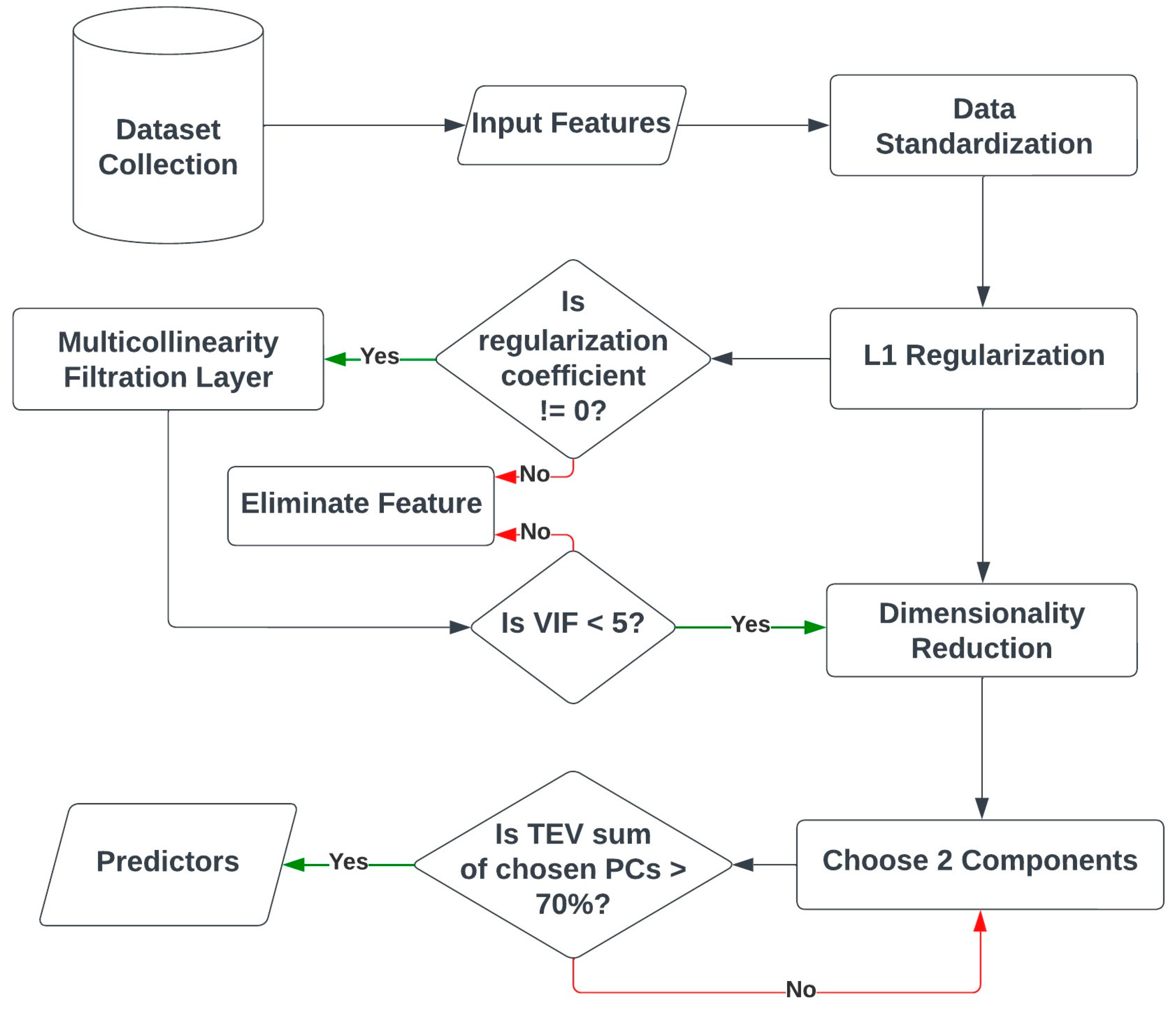
2.2. Preprocessing Phase

The preprocessing phase involves a series of procedures that include normalization, regularization, filtering for multicollinearity, and reducing dimensionality, as shown in Figure 1.

The input features consist of $D_{\sigma }$, $P_L$, $K_F$, ${\sigma }_{EoA}$, ${\sigma }_{EoD}$, ${\sigma }_{AoA}$, ${\sigma }_{AoD}$, and L, where L represents the label of the wireless communication terrestrial scenario. Each row, denoted as $A_i$, corresponds to a single data point, which will undergo Z-score normalization. It is important to normalize the data to handle outliers, as unnormalized data can adversely affect the performance of ML models. Each data point is subjected to the Z-score normalization, $A_i^j$, which determines how far a data point is from the mean divided by the standard deviation and is denoted as [15]

$$A_i^j=\frac{A_i^j-\overline{A^j}}{{\sigma }_{A^j}},$$

(5)

where $\overline{A^j}$ and ${\sigma }_{A^j}$ represent the mean and standard deviation of each feature j.

Next, the normalized data points undergo regularization to eliminate unnecessary features and improve classification performance. The regularization technique used is LASSO, which is a type of L1 regularization known as the least absolute error. The LASSO regression ${\widehat{B}}^{lasso}$, as [16]

$${\widehat{B}}^{lasso}=argmin\left\{\frac{1}{2}{\displaystyle \sum }_{i=1}^N\left(y_i-{\beta }_0-{\displaystyle \sum }_{j=1}^p{x}_{ij}{\beta }_j\right)+\lambda {\displaystyle \sum }_{j=1}^p\left|{\beta }_j\right|\right\},$$

$$\mathit{subject}\mathit{to}{\displaystyle \sum }_{j=1}^p\left|{\beta }_j\right|\le t$$

(6)

where $\lambda$ is the regularization penalty range from 0 to 1. ${\beta }_0$ is a constant coefficient. $\beta =\left({\beta }_0, {\beta }_1,{\beta }_2,\dots ,{\beta }_N\right)$ is the vector coefficient that represents the degree of regularization.

For feature selection enhancement, an added filtration layer based on VIF is followed by the regularization. VIF is a statistical measure used to assess the multicollinearity (high correlation) among predictor variables in a regression model. It helps to determine how much the variance in the estimated regression coefficients is increased due to multicollinearity. VIF is commonly used in ML to identify and eliminate features that may negatively impact the performance and interpretability of the model. The steps of performing VIF calculations are as follows:

• VIF calculation: For each predictor variable in a regression model, the VIF is calculated by regressing that variable against all the other predictor variables. The formula for calculating the VIF of a variable is VIF = 1/(1 − R²), where R² is the coefficient of determination of the regression model.
• Interpreting VIF values: VIF values are always ≥ 1. A VIF of 1 indicates no multicollinearity, whereas a VIF greater than 1 suggests some level of multicollinearity. Generally, a VIF threshold of 5 or 10 is considered significant, indicating high multicollinearity.
• Identifying problematic features: Variables with high VIF values indicate strong multicollinearity with other predictor variables. These variables contribute redundant information to the model and can cause issues, such as unstable coefficient estimates, low interpretability, and inflated standard errors. Thus, they should be identified as potential candidates for elimination.
• Eliminating features: Once high VIF features are identified, they can be eliminated from the model. Removing one or more features with high VIF leads to a reduction in multicollinearity and improves the model stability and interpretability. The specific method of feature elimination depends on the context and goals of the ML problem. It could involve removing one feature at a time or using more advanced techniques, like stepwise regression or regularization methods.

The multicollinearity can be validated through VIF using the method in [17]

$$VIF=\frac{1}{1-R_j^2},$$

(7)

where $R_j^2$ is the multiple $R^2$ for the regression of a feature on the other covariates.

The VIF is a measure of how strongly a predictor variable is related to other predictors in a regression model. A higher VIF indicates lower information entropy, suggesting stronger multicollinearity. Even if a feature has a VIF of 5, it can still be considered highly multicollinear. It is generally advised to avoid VIF values exceeding 10, as this indicates the definite presence of multicollinearity [17].

The final preprocessing step involves dimension projection, which aims to reduce the number of predictors in ML models. This helps in decreasing the computational complexity [18]. The kernel principal component analysis (k-PCA) method is used for this purpose.

Radial basis function (RBF) is the kernel type that is utilized, and it may be represented as [18]

$$\mathsf{{\rm K}}\left(A_a,A_b\right)=exp\left(-\rho {\left|\left|A_a-A_b\right|\right|}^2\right),$$

(8)

Let us assume that there are two distinct points $\left(A_a, A_b\right)$ and a hyper-parameter threshold $\rho$. In this case, one can visualize that the components of the output are determined by the probability density function (PDF).

The principal components are split into training and validation sets following data preparation. The goal is to effectively categorize the four scenarios, RMa LoS, RMa NLoS, UMa LoS, and UMa NLoS. To accomplish this, the classification task is tested using various algorithms: RF, KNN, SVM, and GMM.

RF is a powerful ML algorithm that combines multiple decision trees to achieve accurate predictions by averaging their outcomes. It excels in handling complex data and mitigating overfitting [17]. KNN classifies unknown data points by considering the majority of nearby points based on their closest distances [19]. SVM aims to create distinct support vectors and optimize hyperplanes to minimize errors and maximize margins for each data group [20]. The statistical characteristics of the data are used by the GMM, an unsupervised learning technique, to create clusters [10].

3. Results and Discussion

Here, each step described in the pretreatment and processing methods has its results, which are revealed and provided. The dataset statistics, regularization, VIF filtration, k-PCA, and ML algorithms are evaluated sequentially.

3.1. Dataset Statistics

The dataset provided by the previous work [8,9] was generated through the QuaDRiGa platform Spatial Consistency model [9], which places First Bounce Scatterers (FBSs) and Last Bounce Scatterers (LBSs) randomly. The system model follows the IEEE standards of 38.901.

Table 1. Statistical distribution of original dataset [9].

	RMa LoS	RMa NLoS	Uma LoS	Uma NLoS
DS (dB)	66 + 1.3	72.1 + 0.5	68.2 + 4.2	62 + 1.9
KF (dB)	2.6 + 0.2	3 + 0.05	2.7 + 0.5	3 + 0.05
PL (dB)	0.77 + 1.8	0.84 + 3.5	0.75 + 1.9	0.92 + 3.4
asA (deg)	54.5 + 5.6	21 + 3.2	79.7 + 35	87.4 + 6
asD (deg)	13.8 + 3.3	7 2.3	13.6 + 4	11.6 + 0.8
esA (deg)	3 1.8	2.8 + 0.2	8.9 + 2.4	26 + 3.91
esD (deg)	3.5 + 1.5	1.3 + 0.05	2.7 + 1.7	1 + 0.5

provides statistical information summarizing various scenarios. Each scenario is represented by a set of data points (A_i) consisting of variables, such as $D_{\sigma }$, $P_L$, $K_F$, ${\sigma }_{EoA}$, ${\sigma }_{EoD}$, ${\sigma }_{AoA}$, ${\sigma }_{AoD}$, and L. The index i corresponds to the row number, while L represents the target variable.

3.2. Regularization and VIF Filtration Layer Results

After the data were standardized using the standard scaler of the Z-score method, the mean and standard deviation of each feature become 0 and 1, respectively. Then, the feature selection process takes place using LASSO, as shown in Figure 2.

The DS, asD, and esD are the features to drop since they are considered as noisy data as their regularization coefficients are 0. Then, the VIF filtration layer takes place by removing the features having VIF value greater than 5.

Table 2. VIF filtration layer results.

Feature	KF	PL	asA	esA
VIF Value	1.083771	2.464491	2.483781	5.001260

shows the VIF filtration layer calculations for the remaining features: asA, PL, KF, and esA.

The esA is considered a highly multi-collinear feature, so the filtration layer dropped it. The remaining features, then, are KF, PL, and asA. Compared to the previous work [8,9], this layer, when added to regularization, could drop the features and ensure that there are no multi-collinear features. In conclusion, the enhanced regularization process could reduce the data dimensions from seven to three before performing the PCA. This process outperformed the previous work [8,9], where the dimensionality decreased from seven to four before applying PCA.

3.3. k-PCA Results

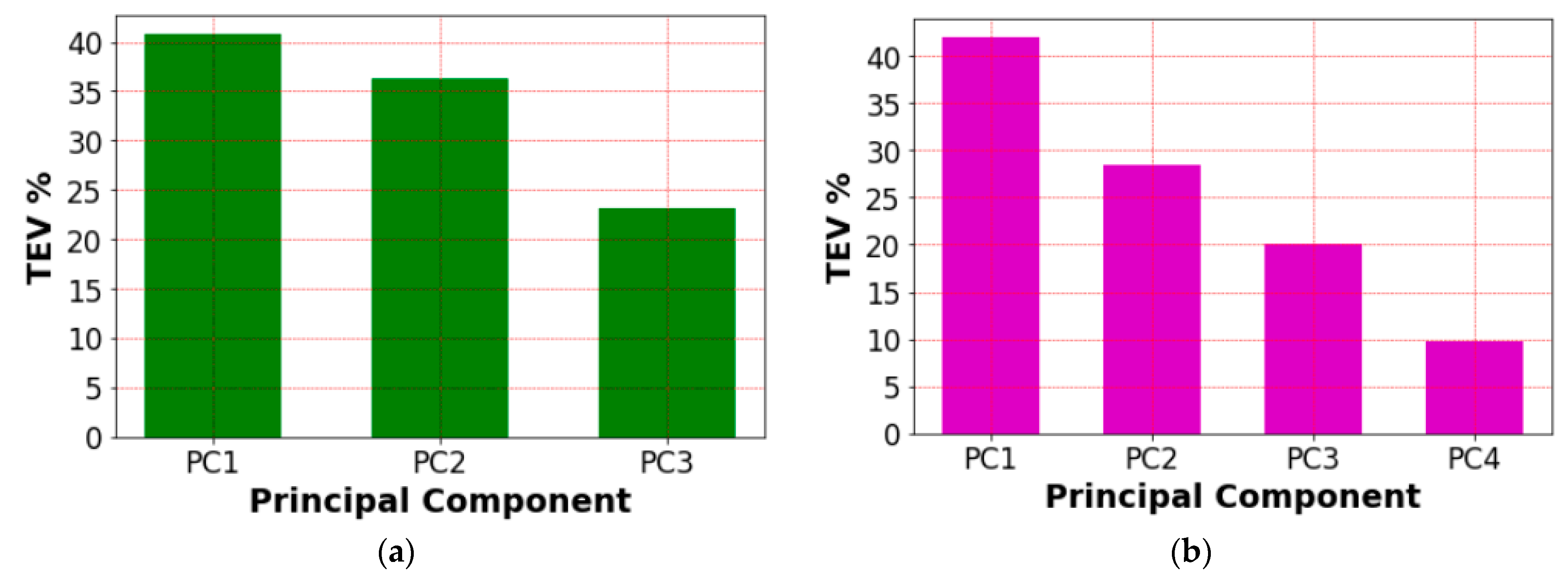
The feature selection process employs regularization and VIF filtration to reduce the dimensionality of the data. This resulted in a decrease from seven to three dimensions, with the VIF filtration removing the esA. Additionally, the use of k-PCA further reduced the data dimensionality. The chosen kernel type for k-PCA is RBF. The total explained variance (TEV) of the k-PCA results is shown in Figure 3.

Based on the sum of the TEV of the first and second components (PC1, PC2), the data dimensionality could be reduced from three to two since the sum of the TEV is 76%. This shows the importance of adding the VIF filtration layer to keep the information gain maximized.

The k-PCA output is illustrated in Figure 4. The PDF of the first principal component, PC1, is displayed in Figure 4a for all possible scenarios. It is evident that PC1 exhibits class overlap, which could lead to misclassification due to the overlapping groups. Both RMA NLoS and UMA NLoS exhibit this overlapping of data. The PDF of the second principal component, PC2, on the other hand, is shown in Figure 4b, and it shows a clear differentiation of information that may be used to separate the four groups. Consequently, PC2 adds a new dimension to the data, enabling easy differentiation between UMa NLoS and RMa LoS.

3.4. Classification Performance

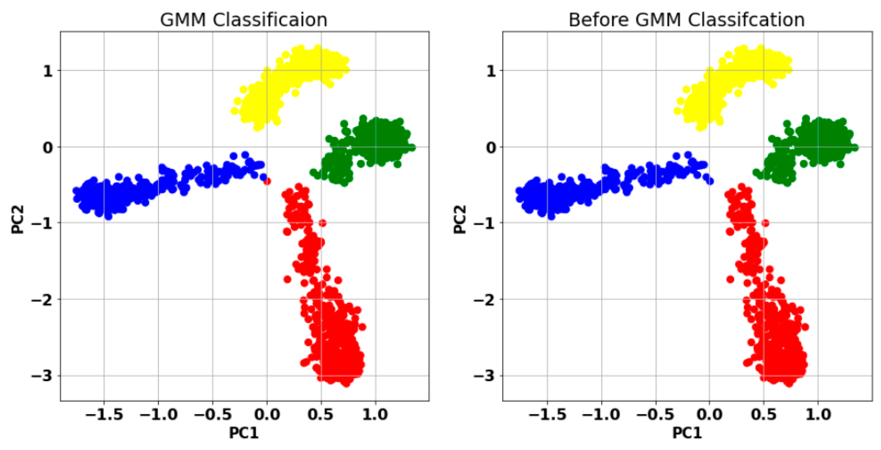
Now, we discuss the results of ML as the last layer of the classification scheme. The effectiveness of the supervised learning algorithms RF, KNN, and SVM is assessed. The clustering time is revealed for the unsupervised learning GMM.

After using the PC1 and PC2 as ML predictors, GMM clustering could achieve 100% classification accuracy, as shown in Figure 5.

The best hyperparameters of GMM obtained are the following: number of components = 4, covariance type = ‘Full’.

The supervised learning algorithms RF, KNN, and SVM achieved a classification accuracy of 100%. The number of neighbors in KNN is trivial since the maximum absolute error (MAE) is always 0. The SVM kernel type used is linear as its computational complexity is minimum. The best hyperparameters obtained for RF that achieved 100% accuracy are as follows: number of estimators = 5, criterion = ‘gini’.

The cross-validation method is used to double check the overfitting. The number of subsets used for training is 10. Each subset achieved a cross-validation score of 100%, resulting in an average of 100% accuracy in each supervised algorithm.

3.5. Result Comparison with Previous Work

In this section, we introduce a comparison between our model and the previous work in terms of the preprocessing and processing phases of ML. As mentioned earlier, the preprocessing phase could reduce the amount of computational complexity of the k-PCA process compared to previous work [8,9].

Table 3. Data preprocessing results comparison.

Model	Regularization	VIF Filtration	Dimension Reduction	TEV
Present work	7 to 4	4 to 3	3 to 2	76%
Work of [8,9]	7 to 4	N/A	4 to 2	72%
Work of [10]	N/A	N/A	7 to 3	71%

represents the different layers of eliminating features and dimension reduction for the proposed and previous work [8,9,10].

Clearly, the proposed model in this paper outperforms the previous models [8,9,10] because the VIF filtration layer could eliminate a noisy feature before performing the dimension reduction. Moreover, the TEV of the remaining two components could reach 76%.

In terms of ML algorithms,

Table 4. Classification accuracy comparison for each algorithm.

Algorithms	RF	KNN	SVM	k-Means	GMM
Work of [8,9]	N/A	99%	99%	97%	98%
Present work	100%	100%	100%	N/A	100%

shows a comparison between this work and the previous work’s accuracy.

The accuracy of each model is increased when compared with the latest work and reaches 100% for KNN, SVM, and GMM.

4. Conclusions

In conclusion, this study focused on the classification of wireless communication channel scenarios and the importance of efficient data preprocessing, particularly in the context of 6G and its multiple scenarios of transmission. By incorporating ML techniques and introducing the variance inflation factor (VIF) elimination as an additional layer to enhance the regularization preprocessing phase, the accuracy of scenario identification was significantly improved. The evaluation of VIF allowed for the removal of highly multi-collinear features after applying an L1 regularization penalty. This approach, combined with ML algorithms, such as RF, KNN, SVM, and GMM, achieves impressive accuracy of 100% for identifying different rural and urban scenarios. Moreover, the TEV achieved in this work is 76%, surpassing the previous state-of-the-art study that achieved a TEV of 71%. This indicates the effectiveness of the proposed methodology in accurately classifying wireless communication channel scenarios. It is worth mentioning that during the VIF filtration process, the angular information of esA was removed from the dataset as it exhibited residual multicollinearity, even after regularization. This highlights the effectiveness of the VIF elimination approach in identifying and mitigating multicollinearity issues in the dataset.

For future work, the employment of AI in more dynamic scenarios is still considered as a rich research area. Classification time optimization is also another hot area of research. In the next research step, new models will be attached such as DDQN-based models [21,22] to tackle the dynamic scenario classification issue while keeping low classification latency.