An Improved LSTNet Approach for State-of-Health Estimation of Automotive Lithium-Ion Battery

Abstract

Accurately estimating the state of health (SOH) of lithium-ion batteries (LIBs) is one of the pivotal technologies to ensure the safe and dependable operation of electric vehicles (EVs). To tackle the challenges related to the intricate preprocessing procedures and extensive data prerequisites of conventional SOH estimation approaches, this paper proposes an improved LSTNet network model. Firstly, the discharged battery sequence data are divided into long-term and short-term sequences. A spatially convolutional long short-term memory network (ConvLSTM) is then introduced to extract multidimensional capacity features. Next, an autoregressive (AR) component is employed to enhance the model’s robustness while incorporating a shortcut connection structure to enhance its convergence speed. Finally, the results of the linear and nonlinear components are fused to make predictive judgments. Experimental comparisons on two datasets are conducted in this study to demonstrate that the method fits the electric capacity recession curve well, even without the preprocessing step. For the data of four NASA batteries, the maximum root mean square error (RMSE), the mean absolute error (MAE), and the mean absolute percentage error (MAPE) of the prediction results were maintained at 0.65%, 0.58%, and 0.435% when the proportion of the training set was 40%, which effectively validates the model’s feasibility and accuracy.

1. Introduction

Lithium-ion batteries (LIBs) are widely used in electric vehicles (EVs), drones, and portable electronic devices due to their advantages of high energy density, high charging efficiency, wide operating temperature range, and long cycle life [1,2]. LIBs are pivotal in powering EVs and determining their performance and reliability [3]. As one of the most critical components of EVs, the battery’s health and longevity significantly impact the driving range, efficiency, and user experience [4]. Accurate assessment of battery health and effective analysis techniques are thus of paramount importance for ensuring optimal vehicle performance, extending battery lifespan, and providing reliable energy storage solutions [5]. SOH estimation techniques for LIBs have the potential to enhance operational efficiency, improve safety, reduce maintenance costs, and enable informed decision-making regarding battery replacement or repair strategies. Therefore, the accurate estimation of battery SOH empowers researchers and industry professionals to optimize the performance and lifespan of automotive batteries, driving the sustainable adoption of EVs and shaping the future of transportation [6].

Currently, there are three main methods for predicting the capacity of LIBs: model-based methods, data-driven methods, and hybrid methods [7,8]. Model-based methods are based on different principles and include electrochemical models, equivalent circuit models, and empirical models [9,10]. Electrochemical models establish corresponding models based on the electrochemical reactions inside the battery and predict the battery life based on other data, such as the current, voltage, and internal resistance. Song et al. [11] constructed an electrochemical model that simulates the charge and discharge of lead-acid batteries and combines them with particle filtering (PF) to obtain good prediction stability. Equivalent circuit models extract features based on charging and discharging voltages in the circuit and then build models based on the least-squares method. However, due to the complex and nonlinear processes of the internal reactions of batteries, it is difficult to reflect the processes accurately using model-based methods. Hence, model-based methods generally require greater robustness and offer an advantage in terms of accuracy [12,13].

With the rapid advancement of computer technology, data-driven methods for predicting the capacity of LIBs have steadily increased prediction accuracy [14]. There are several types of data-driven LIB life prediction methods: support vector machines (SVMs), PF, Gaussian process regression (GPR) [15,16], artificial neural networks (ANNs), recurrent neural networks (RNNs), and long short-term memory (LSTM). Zhang et al. [17] extracted health factors from battery voltage capacity discharge curves and then used a WLS-SVM for prediction. The SVM demonstrates efficient handling of high-dimensional data and strong generalization capability. However, as the dataset size increases, the computational complexity also significantly grows, leading to diminished computational efficiency [18]. Traditional PF suffers from sample degeneracy and impoverishment problems [19,20]. To address this issue, further research was conducted, proposing the use of a heuristic Kalman algorithm in combination with PF to solve these problems [21]. PF can handle non-Gaussian noise in battery life prediction, providing more accurate forecast results. However, the method demands high precision in system modeling and does not completely resolve the issue of particle degeneracy. Moreover, GPR belongs to the category of Bayesian nonparametric methods, enabling it to model intricate systems while systematically managing uncertainty. Dang et al. [22] designed a new kernel function, enabling the GPR to accurately predict capacity values near the training set. This novel kernel function better captures the nonlinear characteristics of battery life, but it also introduces new challenges in model parameter tuning. ANNs are extensively utilized in data-driven methodologies [23]. Nevertheless, this approach is susceptible to the local minimum phenomenon. With the advancement of deep learning, RNNs have achieved good performance in handling time series problems. However, the RNN is prone to the problem of vanishing gradients on long time sequences, rendering it incapable of addressing long-term data dependencies [24]. To tackle this issue, LSTM and GRU have been introduced as enhancements to RNNs. Fasahat et al. [25] introduced an autoencoder–LSTM hybrid approach for improved accuracy in battery state-of-charge estimation. Cheng et al. [20] proposed a model for SOH estimation by integrating empirical pattern decomposition with the backpropagation of LSTM. Chen et al. [26] used five preprocessing methods to construct input data and employed a CNN and LSTM for residual life prediction. Wang et al. [27] improved the FF-LSTM model and designed a unique three-dimensional current, voltage, and temperature change program for verification. These deep learning methods preserve the advantage of a CNN in terms of feature extraction and the sensitivity of LSTM for temporal prediction, which achieves higher prediction stability and accuracy. However, the current deep learning methods for SOH estimation heavily depend on complex preprocessing methods and require sampling or feature extraction from the complete charge and discharge current and voltage curves as input for the model, which is difficult to achieve in practical applications. Moreover, a CNN cannot simultaneously capture both long-term and short-term features of the data, while traditional LSTM models cannot extract spatial features from the data.

Here, we propose an SOH estimation method based on an improved LSTNet network that directly takes battery discharge data as input while considering both the long-term and short-term features of battery capacity data. The proposed method divides the data into long-term and short-term and extracts their features using a 1D-CNN. As this work directly inputs the original charge–discharge information into the model and increases the difficulty of feature extraction, ConvLSTM is used instead of traditional LSTM after dimensionality augmentation, which not only separates noise from the functional features but also enables the model to extract spatial correlations. In order to mitigate the limitations associated with the voluminous output data and the sluggishness in the model training speed, this paper also adds shortcut connection to accelerate model convergence. The proposed method is validated using NASA and MIT LIB datasets under various operating conditions and achieves high accuracy.

The contributions made by this work are summarized below:

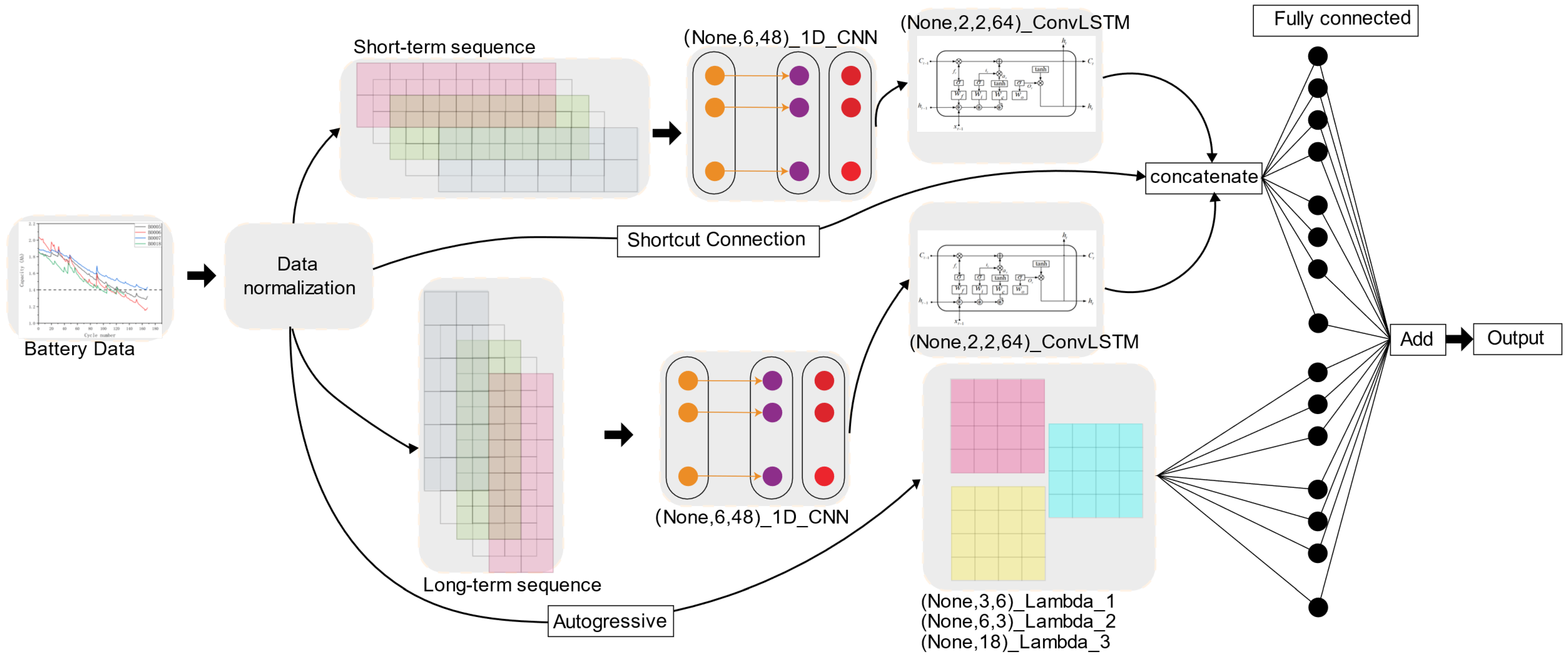
• This paper proposes an approach that directly handles battery capacity data by dividing the raw data into long-term and short-term sequences, thereby effectively learning the hidden features of the original data;
• Due to the complexity of the original data, ConvLSTM is introduced in this study to endow the model with spatial feature analysis capabilities. Shortcut connections are also incorporated to expedite model convergence, improving performance;
• A method for estimating the SOH of automotive LIBs is proposed based on an improved LSTNet. The experimental results demonstrate that the proposed method achieves higher accuracy without extensive preprocessing steps.

2. Methods

LSTNet is a deep learning framework for multivariate time series data, incorporating long- and short-term trends. The structure of the model used in this study is illustrated in Figure 1. The model architecture consists of convolutional layers, ConvLSTM layers, and an autoregressive (AR) component. By separating the long-term trends and short-term periodicity in the time series, LSTNet can improve prediction accuracy and reduce the information loss caused by time series downsampling.

2.1. 1D-CNN

The LSTNet framework first inputs the battery life sequence to a one-dimensional convolutional layer without pooling. This work adds multiple convolutional layers to the LSTNet framework, which mainly strengthens the ability to capture short-term patterns and local dependencies between variables from the time series data. The width of the convolution kernel is denoted as $\omega$, and the height is denoted as $n$ (which is the same as the number of variables). The convolution kernel slides along the one-dimensional data and performs matrix multiplication with the corresponding elements. The 1D-CNN used in this work does not include pooling layers and extracts abstract features from raw data. As shown in Figure 2, the input data size is $m\times n$, and the size of the convolution kernel is $a\times b$. The kernel slides along one direction and performs convolution operations. The width of the kernel needs to be consistent with the width of the input time series. The calculation of the i-th kernel $c_i$ with the input matrix can be represented as:

$$a_i=c_i \ast b_i$$

(1)

In the equation, ∗ denotes the convolution operation, and $b_i$ is the bias term for the convolution.

2.2. ConvLSTM

In this work, the ConvLSTM is used as the recurrent layer of LSTNet to capture long-term information on battery capacity. The recurrent skip component can alleviate the problem of gradient vanishing. ConvLSTM was proposed at the NIPS Conference in 2015 [28]. The authors extended the idea of fully connected LSTM networks to ConvLSTM, replacing the feedforward method from Hadamard product to convolution and changing the transformation from input-to-state and state-to-state to convolution operations. Therefore, ConvLSTM can capture not only temporal correlations but also spatial correlations. The structure of ConvLSTM is illustrated in Figure 3, and its calculation formulas are as follows:

$$I_t=\sigma \left(w_{di}\ast D_t+w_{hi}^{}\ast H_{t-1}+w_{ci}{}^{}\circ C_{t-1}+b_i\right)$$

(2)

$$F_t=\sigma \left(w_{df}\ast D_t+w_{hf}\ast H_{t-1}+w_{cf}\circ C_{t-1}+b_f\right)$$

(3)

$$C_t=F_t^{}\circ C_{t-1}+I_t{}^{}\circ \mathrm{t}\mathrm{a}\mathrm{n}\mathrm{h}\left(w_{dc}\ast D_t+\left.w_{hc}\ast H_{t-1}+b_c\right)\right.$$

(4)

$$O_t=\sigma \left(w_{do}\ast D_t+w_{ho}\ast H_{t-1}+w_{co}{\circ }^{}{C}_t+b_o\right)$$

(5)

$$H_t=O_t^{}\circ \mathrm{t}\mathrm{a}\mathrm{n}\mathrm{h}\left(C_t\right)$$

(6)

In the equations, $D_t$ is the input; $w$ and $b$ are learnable parameters; $\sigma$ is the nonlinear activation function; ‘∗’ represents convolution, and ‘∘’ represents the Hadamard product. $C_t$ is the memory cell used to store state information, $I_t$ is the input gate, $F_t$ is the forget gate, and $O_t$ is the output gate.

2.3. Fully Connected Layer and AR Model

The data are finally fed into a fully connected layer to obtain the output. The input to the fully connected layer consists of two parts: one is the output of the recurrent and recurrent skip layers, and the other is the output of the AR layer. As the convolutional and recurrent layers do not have linear characteristics, and the changes in battery capacity data are often irregular, the neural network model is insensitive to the input of battery capacity data, leading to an increase in error in the prediction. To address this issue, the LSTNet framework adopts a traditional AR model as a linear branch in the LSTNet model. The model results are as follows:

$$h_{t,i}^L={\sum }_{k=0}^{q^{\alpha r}-1} W_k^{\alpha r}{y}_{t-k,i}+b^{\alpha r}$$

(7)

In the equation, $h_{t,i}^L$ is the predicted result of the AR model, and $q^{\alpha r}$ is the window size.

2.4. Shortcut Connection

Shortcut connection is a structure in residual networks mainly used to solve the problems of gradient vanishing and gradient explosion during neural network training, accelerate model training, and improve model performance. Considering the large amount of input data and the difficulty of model training in this work, the shortcut connection module is introduced to accelerate the convergence speed of the model. In the traditional structure of neural networks, the output of each layer depends only on its input and weights. In shortcut connection, each layer’s output also includes the previous layers’ output. In this work, shortcut connection is primarily employed to pass the output of the preceding layers, ensuring that the magnitude of the gradient is preserved. This enables the network to learn important features more efficiently and converge more rapidly. The basic structure of the shortcut connection module is shown in Figure 4.

3. Results and Discussion

The experimental platform for this study consisted of an Intel I5-12400F CPU, a GTX1080 graphics card, and 32 GB of dual-channel memory. The programming language used was Python and its version is 3.6.4, with TensorFlow version 1.13.1, and the operating system was Windows 10.

3.1. Experimental Setup

3.1.1. Dataset Introduction

The dataset used in this study is the NASA battery dataset [29]. The reasons for selecting the NASA LIB dataset for battery life prediction are as follows:

• Data Reliability: The NASA LIB dataset, provided by the National Aeronautics and Space Administration, exhibits high reliability and authenticity. This dataset is carefully collected and recorded, encompassing battery operational data from various real-world applications and environmental conditions. It provides meaningful training and evaluation data for battery life prediction models;
• High Dimensionality and Richness: The NASA LIB dataset typically includes a wealth of sensor measurements, such as current, voltage, and temperature, as well as battery state information, such as charge status and capacity degradation. These high-dimensional and rich data provide comprehensive feature information that aids in developing accurate battery life prediction models;
• Academic Reference: The NASA LIB dataset is widely used in academic research and has become a benchmark test dataset for battery life prediction algorithms and models. Choosing this dataset ensures the comparability of research results and enables comparison and validation against the work of other researchers.

NASA utilizes 18650 LIBs as the research objects to develop high-power LIBs for addressing the power issues in hybrid EVs. Accelerated life experiments were conducted on an LIB accelerated life test platform, resulting in a series of NASA data. The test platform includes programmable electronic loads, DC power supplies, thermostats, sensors, data acquisition systems, and electrochemical impedance spectroscopy analyzers. Taking the first group of batteries as an example, the charging experiment was conducted at an ambient temperature of 24 °C. The batteries were charged with a constant current of 1.5 A until the terminal voltage reached 4.2 V and then switched to constant voltage charging until the charging current dropped to 20 mA, indicating the end of the charging process. The discharge experiment was conducted at an ambient temperature of 24 °C, where batteries B0005, B0006, B0007, and B0018 were discharged at a constant current of 2 A until the terminal voltage of each battery reached 2.7 V, 2.5 V, 2.2 V, and 2.5 V, respectively. Figure 5 shows the capacity degradation curves of batteries B0005, B0007, B0006, and B0018.

3.1.2. Experimental Data and Parameter Settings

In this study, the NASA dataset was used and preprocessed. The data were divided into training and testing sets, where 60%, 50%, and 40% of the data were allocated to the training set, and the corresponding 40%, 50%, and 60% were allocated to the testing set. The training set was fed into the LSTNet network model for training. The input dimension of the model in this study was 6, and the output dimension was 1. It included two inputs, two 1D-CNNs, one recurrent layer, one skip layer, and two fully connected layers. The number of filters in the two convolutional layers was set to 48, the kernel size was 3, and the stride was 1. The number of skip connections was 3, the high window was 3, the dropout coefficient was 0.5, and the number of epochs was 300. These parameters were obtained using a grid search algorithm, and the structure and parameters of the predictive model are shown in Figure 3.

To demonstrate the superiority of the LSTNet model, several other models, including LSTM, GRU, CNN-GRU, WD-2DCNN, and BLS-LSTM [20,26], were selected for comparison and validation. Considering the limited feature extraction capability of traditional models, the input data for these models underwent simple preprocessing to obtain the average degradation trend of capacity. The selection of these models was based on the following factors:

• Selecting LSTM and GRU models to evaluate whether the proposed model outperforms commonly used LSTM models and their variants;
• Selecting a CNN-LSTM to verify whether the proposed model is superior to structurally similar network models;
• Selecting a WD-2DCNN and BLS-LSTM to evaluate whether the proposed model outperforms methods with preprocessing steps.

The LSTM, GRU, CNN-GRU, and LSTNet model structures used in this study are compared in

Table 1. The structure of prediction models.

Method	Hidden Layer Structure	Hidden Layer Settings	Dropout	Filter Size	Optimizer	Batch size
LSTM	One LSTM layer and one dense layer	LSTM nodes: 100 and fully connected layer nodes: none, 1	0.5	-	Adam	8
GRU	One GRU layer and one dense layer	GRU nodes: 100 and fully connected layer nodes: none, 1	0.5	-	Adam	8
CNN_GRU	One 1D-CNN, one max-pooling, one GRU, and one fully connected layer	The number of filters is 48, GRU nodes: 100, and fully connected layer nodes: none, 1	0.5	3	Adam	8
LSTNet	As shown in Figure 1	The number of filters is 48, GRU nodes: 64, and fully connected layer nodes: none, 1	0.5	3	Adam	8

.

3.2. Model Evaluation Indicators

In this work, the mean absolute error (MAE), root mean squared error (RMSE), and mean absolute percentage error (MAPE) were used as performance evaluation metrics for the models. Smaller values of MAE, MAPE, and RMSE indicate higher precision of the prediction results. The definitions of these performance metrics are as follows:

$$\mathrm{M}\mathrm{A}\mathrm{E}=\frac{1}{n}{\sum }_{i=1}^n \left|y_i-{\widehat{y}}_i\right|$$

(8)

$$\mathrm{R}\mathrm{M}\mathrm{S}\mathrm{E}=\sqrt{\frac{1}{n}{\sum }_{i=1}^n {\left(y_i-{\widehat{y}}_i\right)}^2}$$

(9)

$$\mathrm{M}\mathrm{A}\mathrm{P}\mathrm{E}=\frac{\mathrm{100\%}}{n}{\sum }_{i=1}^n \left|\frac{{\widehat{y}}_i-y_i}{y_i}\right|$$

(10)

In the equations, $n$ represents the number of instances in the test set, $y_i$ is the actual value of the i-th instance in the test set, and $\widehat{y}$ is the predicted value of the i-th instance in the test set.

3.3. Experimental Results and Comparative Analysis

3.3.1. Comparison with Traditional Models

Table 2. The predictive evaluation results for different models.

Battery Number	Percentage of Training Set	Method	RMSE	MAE	MAPE
B0005	50%	LSTM	0.01732	0.01592	0.01161
		GRU	0.02247	0.01888	0.01393
		CNN-GRU	0.01620	0.01298	0.00962
		LSTNet	0.00492	0.00313	0.00232
	40%	LSTM	0.01246	0.00972	0.00715
		GRU	0.01078	0.00797	0.00586
		CNN-GRU	0.00341	0.00254	0.00182
		LSTNet	0.00563	0.00369	0.00261
	60%	LSTM	0.00935	0.00775	0.00579
		GRU	0.00549	0.00425	0.00319
		CNN-GRU	0.00806	0.00773	0.00560
		LSTNet	0.00064	0.00051	0.00038
B0006	50%	LSTM	0.01435	0.01360	0.01022
		GRU	0.01079	0.01042	0.00783
		CNN-GRU	0.03268	0.03132	0.02389
		LSTNet	0.00370	0.00180	0.00146
	40%	LSTM	0.02107	0.01885	0.01436
		GRU	0.01303	0.01097	0.00847
		CNN-GRU	0.04118	0.03821	0.02890
		LSTNet	0.00650	0.00580	0.00435
	60%	LSTM	0.00902	0.00723	0.00566
		GRU	0.00927	0.00698	0.00563
		CNN-GRU	0.00853	0.00710	0.00549
		LSTNet	0.00193	0.00116	0.00090
B0007	50%	LSTM	0.02158	0.01806	0.01234
		GRU	0.02191	0.02015	0.01364
		CNN-GRU	0.01769	0.01572	0.01065
		LSTNet	0.00218	0.00085	0.00059
	40%	LSTM	0.01479	0.01177	0.00800
		GRU	0.01746	0.01431	0.00972
		CNN-GRU	0.00597	0.00489	0.00327
		LSTNet	0.00261	0.00129	0.00086
	60%	LSTM	0.00526	0.00491	0.00334
		CNN-GRU	0.00744	0.00625	0.00414
		GRU	0.00617	0.00503	0.00346
		LSTNet	0.00339	0.00127	0.00090
B0018	50%	LSTM	0.00324	0.00287	0.00202
		GRU	0.00341	0.00330	0.00233
		CNN-GRU	0.00505	0.00462	0.00324
		LSTNet	0.00059	0.00026	0.00018
	40%	LSTM	0.00925	0.00883	0.00619
		GRU	0.00236	0.00195	0.00137
		CNN-GRU	0.00830	0.00783	0.00547
		LSTNet	0.00145	0.00052	0.00037
	60%	LSTM	0.00191	0.00169	0.00121
		GRU	0.00239	0.00222	0.00158
		CNN-GRU	0.00280	0.00255	0.00181
		LSTNet	0.00602	0.00349	0.00255

presents the prediction results of different models on NASA datasets B0005, B0007, B0006, and B0018 under various operating conditions. Figure 6 shows the fitting performance of the predicted and actual values of the batteries under different operating conditions. Figure 6 compares the fitting performance of different models on NASA datasets B0005, B0007, B0006, and B0018 under various operating conditions. Figure 7 shows the plot of the capacity prediction error for different methods.

This study conducted multiple experiments on the network models mentioned above, and the obtained prediction values may have some fluctuations. They consider various factors, such as practical application; the smaller the MAE, MAPE, and RMSE values, the higher the model prediction accuracy. Analyzing Table 2 and considering the prediction data of multiple batteries, it can be concluded that the LSTM model has the highest prediction accuracy when the dataset is split into 6:4. The maximum and minimum values of RMSE are 2.158% and 0.191%, respectively. In comparison, the MAE’s maximum and minimum values are 1.885% and 0.169%, respectively. The MAPE’s maximum and minimum values are 1.436% and 0.121%, respectively.

Based on the analysis of Figure 7, the LSTM prediction model cannot accurately describe the degradation trend of battery capacity in most operating conditions. Similarly, the GRU model has the highest prediction accuracy when the dataset is divided into 6:4. Its RMSE ranges from 2.247% to 0.236%, its MAE ranges from 2.015% to 0.195%, and its MAPE ranges from 1.393% to 0.137%. Despite being an improved structure of LSTM, GRU’s prediction accuracy for LIBs is similar to that of LSTM. The CNN-GRU model uses a 1D-CNN to extract deep features of the data and combines it with the GRU, which can analyze unidirectional time series. Compared with the GRU model, the fitting degree of the CNN-GRU model has been improved in some operating conditions. Similarly, the CNN-GRU model has the highest prediction accuracy when the dataset is divided into 6:4. Its RMSE ranges from 4.118% to 0.280%, its MAE ranges from 3.821% to 0.254%, and its MAPE ranges from 2.89% to 0.181%. The evaluation indicators of the CNN-GRU model show more significant fluctuations. In conclusion, traditional models rely more on a large amount of data for training, and under a more significant proportion of training sets, traditional models tend to achieve better prediction results.

The proposed model divides the battery capacity sequence into long-term and short-term sequences, extracting features using 1D-CNN layers and utilizing a linear AR model to extract long-term and short-term features of the battery capacity sequence, adding the linear component dramatically improves the prediction accuracy, which can accurately reflect the overall degradation trend of the battery.

Table 3. Errors at extreme hyperparameters.

Method	Number of Neurons	Batch Size	Epoch	RMSE	MAE	MAPE
LSTNet	8	4	20	0.00969	0.00649	0.00483
	128	64	300	0.01064	0.00661	0.00496
	8	4	300	0.00916	0.00534	0.00404
	8	64	300	0.01136	0.00709	0.00534
	8	64	20	0.01295	0.00814	0.00613
	128	64	20	0.01418	0.00931	0.00698
	128	4	20	0.00918	0.00690	0.00511
	128	4	300	0.00927	0.00576	0.00341
	64	8	300	0.00492	0.00313	0.00232
CNN-GRU	8	4	20	0.16497	0.12308	0.07404
	128	64	300	0.02195	0.02162	0.01548
	8	4	300	0.04300	0.03624	0.02667
	8	64	300	0.01992	0.01585	0.01171
	8	64	20	0.30365	0.29070	0.21020
	128	64	20	0.16846	0.15989	0.11581
	128	4	20	0.03641	0.03505	0.02453
	128	4	300	0.06779	0.05828	0.04281
	64	8	300	0.01620	0.01298	0.00962

presents the evaluation indicators of the proposed model, where the minimum RMSE is 0.059%, the minimum MAE is 0.026%, and the minimum MAPE is 0.018%, all of which are lower than the minimum values of the other three traditional models. The highest accuracy is achieved in the B0018 battery with a 4:6 split dataset condition. Under the B0006 battery condition with a 4:6 split dataset, the prediction accuracy of the proposed model is relatively poor, with a minimum RMSE of 0.65%, a minimum MAE of 0.58%, and a minimum MAPE of 0.435%. However, it is still significantly better than the three traditional models. Figure 7 compares multiple evaluation indicators of the B0005 battery, and Figure 8 shows the absolute error plot of the B0005 battery.

Based on the analysis of Figure 8, the proposed method has relatively good prediction accuracy in the front part of the test set, with the absolute error of most prediction points being less than 0.005, which proves that the proposed method can effectively extract hidden features of the training set. The absolute error in the back part of the test set fluctuates greatly, which may be due to the significant difference between the capacity attenuation features of the battery at the end of life and those used for training, leading to a decrease in prediction accuracy. The proposed method directly uses battery discharge data as input. It utilizes the ability of ConvLSTM to extract multidimensional features, which can extract relevant features from data with a large amount of noise. Compared with traditional models, it has higher accuracy in most operating conditions.

3.3.2. Sensitivity Analysis

Sensitivity analysis plays a crucial role in neural network research, enabling researchers to gain deeper insights into the behavior and performance of neural network models. In this section, we conducted a sensitivity analysis of the model, focusing on the impact of different model parameters on the model’s results. To facilitate comparison with traditional models, we performed multiple experiments with varying values of the number of recurrent network neurons, batch size, and Epoch. The initial values of these parameters are shown in Table 1. In this section, we used the B0005 battery from the NASA dataset, with a 5:5 ratio between the training and test sets.

To investigate whether small variations in hyperparameters have a significant impact on the model’s output, we first kept the other hyperparameters constant and varied the number of recurrent network neurons = [8, 16, 32, 64, 128]. Similarly, we selected batch sizes = [4, 8, 16, 32, 64] and Epoch values = [20, 50, 100, 200, 300]. The experimental results are shown in Figure 9.

Analyzing Figure 9, it is evident that the number of neurons, batch size, and Epoch in the CNN-GRU model significantly impact the prediction error. However, in the proposed model, the influence of these three hyperparameters on the prediction results is considerably smaller. Specifically, in the first set of experiments, due to variations in the number of neurons, the maximum RMSE of the proposed model is 2.19 times the minimum RMSE, while the maximum RMSE for CNN-GRU is 3.76 times the minimum RMSE. In the second set of experiments with different batch sizes, the maximum RMSE of the proposed model is 2.72 times the minimum RMSE, whereas for CNN-GRU, the maximum RMSE is 4.08 times the minimum RMSE. In the third set of experiments with varying Epoch values, the maximum RMSE of the proposed model is 2.55 times the minimum RMSE, while for CNN-GRU, the maximum RMSE is 1.83 times the minimum RMSE. Based on the analysis above, the proposed model exhibits higher stability compared to the CNN-GRU model.

To test the stability of the model under extreme conditions, we conducted comparative experiments using a representative set of multiple hyperparameters. The experimental results are presented in Table 3.

Analyzing Table 3, the proposed model maintains an RMSE within 0.01418, MAE within 0.00931, and MAPE within 0.00698 under extreme conditions. On the other hand, CNN-GRU is more sensitive to variations in the model parameters, with an RMSE of 0.30364, MAE of 0.2907, and MAPE of 0.2102 under extreme parameter settings. In conclusion, the proposed model exhibits higher stability and is less sensitive to parameter variations, maintaining higher accuracy in most cases.

3.3.3. Comparison with Advanced Methods

To further demonstrate the advantages of the battery life prediction method proposed in this work, we compared its results with the models proposed in the recent relevant literature using the same dataset. The comparison results are shown in

Table 4. The comparison results of different methods.

Battery Number	Percentage of Training Set	Method	RMSE	MAE
B0005	40%	WD-2DCNN	0.0102	0.0065
		BLS-LSTM	-	-
		LSTNet	0.00563	0.00369
	50%	WD-2DCNN	0.0103	0.0045
		BLS-LSTM	0.0067	0.0069
		LSTNet	0.00492	0.00313
B0006	40%	WD-2DCNN	0.0215	0.0154
		BLS-LSTM	-	-
		LSTNet	0.00650	0.00580
	50%	WD-2DCNN	0.0106	0.0102
		BLS-LSTM	0.0055	0.0067
		LSTNet	0.00370	0.00180
B0007	40%	WD-2DCNN	0.0098	0.0045
		BLS-LSTM	-	-
		LSTNet	0.00261	0.00129
	50%	WD-2DCNN	0.0089	0.0061
		BLS-LSTM	-	-
		LSTNet	0.00218	0.00085
B0018	40%	WD-2DCNN	0.0114	0.0063
		BLS-LSTM	-	-
		LSTNet	0.00145	0.00052
	50%	WD-2DCNN	0.0072	0.0102
		BLS-LSTM	-	-
		LSTNet	0.00059	0.00026

. In reference [30], wavelet packet decomposition was used for preprocessing the initial battery data, and the network was subjected to multiple error corrections, resulting in higher prediction accuracy. In reference [31], a fusion neural network was constructed using the generalized learning system and LSTM. The proposed method in this paper achieved relatively high accuracy while reducing the preprocessing steps.

Table 4 details the training results for the four batteries under various operating conditions. The proposed method has only 8.19% of the RMSE value and 2.5% of the MAE value of the WD-2DCNN when it performs the best. The proposed method has high prediction accuracy and stability under various operating conditions.

3.4. Generalizability Verification

To further demonstrate the adaptability of the proposed method to different battery datasets, we selected the LIB dataset from the Massachusetts Institute of Technology (MIT) [32]. This dataset has a short sampling interval and many sampling points, making it more difficult to extract features directly. For this experiment, we selected two batteries from Channel 5 (CH5) and Channel 10 (CH10), which are A123 Systems company (APR18650M1A) manufactured lithium iron phosphate (LFP)/graphite batteries [33,34], with a nominal capacity of 1.1 Ah and a nominal voltage of 3.3V. The experiments were conducted in a temperature-controlled chamber at 30 °C with a discharge rate of 4 C.

According to the analysis in

Table 5. Prediction results for the MIT dataset.

Battery Number	Percentage of Training Set	Method	RMSE	MAE	MAPE
CH5	40%	LSTNet	0.004878	0.004483	0.004939
	50%		0.004972	0.004751	0.005253
CH10	40%	LSTNet	0.011803	0.010935	0.010024
	50%		0.011642	0.010217	0.011529

, the proposed method achieved a maximum RMSE of 1.6803%, an MAE of 1.4935%, and an MAPE of 1.6024% when using the MIT dataset. The minimum RMSE was 0.4879%, the MAE was 0.4483%, and the MAPE was 0.4939%. The proposed method performed well in different operating conditions, indicating its ability to accurately extract the battery capacity degradation trend even with a short sampling interval and large data volume, achieving good prediction performance.

4. Conclusions

Battery life prediction is crucial in mitigating battery failure rates, enhancing reliability and safety, and optimizing cost savings. This paper proposes an improved LSTNet SOH estimation method for LIBs. In general, the appropriate preprocessing can generate effective factors with higher relevance. However, it may result in a substantial loss of detailed data. In this study, we maintain the entirety of the input data and employ ConvLSTM to extract the multidimensional features, thereby enabling the acquisition of a broader set of capacity degradation trend features. Subsequently, the model performance is rigorously evaluated through experiments, demonstrating its remarkable prediction accuracy and stability.

The improved LSTNet model has higher prediction accuracy than LSTM, GRU, CNN-LSTM, and most denoising algorithms–traditional model frameworks. At a 60% training set ratio, the lowest RMSE is 0.064%, reducing the data preprocessing steps and improving the prediction accuracy. The lowest RMSE is only 7.94% against CNN-GRU, and it has high accuracy in the early stage of the test data. The absolute error of most data points is below 0.005. The proposed method can extract compelling features from the original discharge data and has higher stability.

References

1. Wang, S.; Jin, S.; Bai, D.; Fan, Y.; Shi, H.; Fernandez, C. A Critical Review of Improved Deep Learning Methods for the Remaining Useful Life Prediction of Lithium-ion Batteries. Energy Rep. 2021, 7, 5562–5574. [Google Scholar] [CrossRef]
2. Wang, J.; Zhang, C.; Zhang, L.; Su, X.; Zhang, W.; Li, X.; Du, J. A Novel Aging Characteristics-based Feature Engineering for Battery State of Health Estimation. Energy 2023, 273, 127169. [Google Scholar] [CrossRef]
3. Locorotondo, E.; Corti, F.; Pugi, L.; Berzi, L.; Reatti, A.; Lutzemberger, G. Design of a Wireless Charging System for Online Battery Spectroscopy. Energies 2021, 14, 218. [Google Scholar] [CrossRef]
4. Luo, K.; Chen, X.; Zheng, H.; Shi, Z. A Review of Deep Learning Approach to Predicting the State of Health and State of Charge of Lithium-ion Batteries. J. Energy Chem. 2022, 74, 159–173. [Google Scholar] [CrossRef]
5. Abdelhafiz, S.M.; Fouda, M.E.; Radwan, A.G. Parameter Identification of Li-ion Batteries: A Comparative Study. Electronics 2023, 12, 1478. [Google Scholar] [CrossRef]
6. Xiong, R.; Zhang, Y.; Wang, J.; He, H.; Peng, S.; Pecht, M. Lithium-Ion Battery Health Prognosis Based on a Real Battery Management System Used in Electric Vehicles. IEEE Trans. Veh. Technol. 2019, 68, 4110–4121. [Google Scholar] [CrossRef]
7. Zheng, Y.; He, F.; Wang, W. A Method to Identify Lithium Battery Parameters and Estimate SOC Based on Different Temperatures and Driving Conditions. Electronics 2019, 8, 1391. [Google Scholar] [CrossRef] [Green Version]
8. Lee, H.; Park, J.; Kim, J. Incremental Capacity Curve Peak Points-Based Regression Analysis for the State-of-Health Prediction of a Retired LiNiCoAlO2 Series/Parallel Configured Battery Pack. Electronics 2019, 8, 1118. [Google Scholar] [CrossRef] [Green Version]
9. Xiong, W.; Xu, G.; Li, Y.; Zhang, F.; Ye, P.; Li, B. Early prediction of lithium-ion battery cycle life based on voltage-capacity discharge curves. J. Energy Storage 2023, 62, 106790. [Google Scholar] [CrossRef]
10. Xing, J.; Zhang, H.; Zhang, J. Remaining useful life prediction of Lithium batteries based on principal component analysis and improved Gaussian process regression. Int. J. Electrochem. Sci. 2023, 18, 100048. [Google Scholar] [CrossRef]
11. Song, K.; Hu, D.; Tong, Y.; Yue, X. Remaining life prediction of lithium-ion batteries based on health management: A review. J. Energy Storage 2023, 57, 106193. [Google Scholar] [CrossRef]
12. Zhang, Y.; Ma, H.; Wang, S.; Li, S.; Guo, R. Indirect prediction of remaining useful life for lithium-ion batteries based on improved multiple kernel extreme learning machine. J. Energy Storage 2023, 64, 107181. [Google Scholar] [CrossRef]
13. Zhou, Z.; Liu, Y.; You, M.; Xiong, R.; Zhou, X. Two-stage aging trajectory prediction of LFP lithium-ion battery based on transfer learning with the cycle life prediction. Green Energy Intell. Transp. 2022, 1, 100008. [Google Scholar] [CrossRef]
14. Kim, S.; Yi, Z.; Kunz, M.R.; Dufek, E.J.; Tanim, T.R.; Chen, B.-R.; Gering, K.L. Accelerated battery life predictions through synergistic combination of physics-based models and machine learning. Cell Rep. Phys. Sci. 2022, 3, 101023. [Google Scholar] [CrossRef]
15. Fei, Z.; Zhang, Z.; Yang, F.; Tsui, K.-L. A deep attention-assisted and memory-augmented temporal convolutional network based model for rapid lithium-ion battery remaining useful life predictions with limited data. J. Energy Storage 2023, 62, 106903. [Google Scholar] [CrossRef]
16. Pham, T.; Truong, L.; Bui, H.; Tran, T.; Garg, A.; Gao, L.; Quan, T. Towards Channel-Wise Bidirectional Representation Learning with Fixed-Point Positional Encoding for SoH Estimation of Lithium-Ion Battery. Electronics 2023, 12, 98. [Google Scholar] [CrossRef]
17. Zhang, C.; Wang, H.; Wu, L. Life Prediction Model for Lithium-ion Battery Considering Fast-charging Protocol. Energy 2023, 263, 126109. [Google Scholar] [CrossRef]
18. Duong, P.L.T.; Raghavan, N. Heuristic Kalman Optimized Particle Filter for Remaining Useful Life Prediction of Lithium-ion Battery. Microelectron. Reliab. 2018, 81, 232–243. [Google Scholar] [CrossRef]
19. Zhang, H.; Miao, Q.; Zhang, X.; Liu, Z. An improved unscented particle filter approach for lithium-ion battery remaining useful life prediction. Microelectron. Reliab. 2018, 81, 288–298. [Google Scholar] [CrossRef]
20. Cheng, G.; Wang, X.; He, Y. Remaining useful life and state of health prediction for lithium batteries based on empirical mode decomposition and a long and short memory neural network. Energy 2021, 232, 121022. [Google Scholar] [CrossRef]
21. Lyu, C.; Lai, Q.; Ge, T.; Yu, H.; Wang, L.; Ma, N. A Lead-acid Battery’s Remaining Useful Life Prediction by Using Electrochemical Model in the Particle Filtering Framework. Energy 2016, 120, 975–984. [Google Scholar] [CrossRef]
22. Dang, W.; Liao, S.; Yang, B.; Yin, Z.; Liu, M.; Yin, L.; Zheng, W. An Encoder-decoder Fusion Battery Life Prediction Method Based on Gaussian Process Regression and Improvement. J. Energy Storage 2023, 59, 106469. [Google Scholar] [CrossRef]
23. Zhai, X.; Wang, K.; Peng, N.; Wang, K.; Peng, N.; Zhang, X. Synchronous estimation of state of health and remaining useful lifetime for lithium-ion battery using the incremental capacity and artificial neural networks. J. Energy Storage 2019, 26, 100951. [Google Scholar] [CrossRef]
24. Zhao, G.; Liu, Y.; Liu, G.; Jiang, S.; Hao, W. State-of-charge and state-of-health estimation for lithium-ion battery using the direct wave signals of guided wave. J. Energy Storage 2021, 39, 102657. [Google Scholar] [CrossRef]
25. Fasahat, M.; Manthouri, M. State of charge estimation of lithium-ion batteries using hybrid autoencoder and long short term memory neural networks. J. Power Sources 2020, 469, 228375. [Google Scholar] [CrossRef]
26. Chen, D.; Zhang, W.; Zhang, C.; Sun, B.; Cong, X.; Wei, S.; Jiang, J. A novel deep learning-based life prediction method for lithium-ion batteries with strong generalization capability under multiple cycle profiles. Appl. Energy 2022, 327, 120114. [Google Scholar] [CrossRef]
27. Wang, S.; Takyi-Aninakwa, P.; Jin, S.; Yu, C.; Fernandez, C.; Stroe, D.-I. An improved feedforward-long short-term memory modeling method for the whole-life-cycle state of charge prediction of lithium-ion batteries considering current-voltage-temperature variation. Energy 2022, 254, 124224. [Google Scholar] [CrossRef]
28. Shi, X.; Chen, Z.; Wang, H.; Yeung, D. Convolutional LSTM network: A machine learning approach for precipitation nowcasting. Adv. Neural Inf. Process. Syst. 2015, 28, 802–810. [Google Scholar] [CrossRef]
29. Goebel, B.S.A.K. Battery data set. In NASA Prognostics Data Repository; NASA Ames Research Center: Moffett Field, CA, USA, 2007. [Google Scholar]
30. Ding, P.; Liu, X.; Li, H.; Huang, Z.; Zhang, K.; Shao, L.; Abedinia, O. Useful life prediction based on wavelet packet decomposition and two-dimensional convolutional neural network for lithium-ion batteries. Renew. Sustain. Energy Rev. 2021, 148, 111287. [Google Scholar] [CrossRef]
31. Zhao, S.; Zhang, C.; Wang, Y. Lithium-ion battery capacity and remaining useful life prediction using board learning system and long short-term memory neural network. J. Energy Storage 2022, 52, 104901. [Google Scholar] [CrossRef]
32. Severson, K.A.; Attia, P.M.; Jin, N.; Perkins, N.; Jiang, B.; Yang, Z.; Chen, M.H.; Aykol, M.; Herring, P.K.; Fraggedakis, D.; et al. Data-driven prediction of battery cycle life before capacity degradation. Nat. Energy 2019, 4, 383–391. [Google Scholar] [CrossRef] [Green Version]
33. Clerici, D.; Mocera, F.; Somà, A. Electrochemical–mechanical multi-scale model and validation with thickness change measurements in prismatic lithium-ion batteries. J. Power Sources 2022, 542, 231735. [Google Scholar] [CrossRef]
34. Attia, P.M.; Grover, A.; Jin, N.; Severson, K.A.; Markov, T.M.; Liao, Y.-H.; Chen, M.H.; Cheong, B.; Perkins, N.; Yang, Z.; et al. Closed-loop optimization of fast-charging protocols for batteries with machine learning. Nature 2020, 578, 397–402. [Google Scholar] [CrossRef] [PubMed] [Green Version]
Figure 1. LSTNet structure diagram.
Electronics 12 02647 g001
Figure 2. Schematic diagram of convolution calculation.
Electronics 12 02647 g002
Figure 3. ConvLSTM structure diagram. (‘∗’ represents convolution, ‘×’ represents the Hadamard product).
Electronics 12 02647 g003
Figure 4. Shortcut connection structure.
Electronics 12 02647 g004
Figure 5. NASA dataset’s four sets of battery capacity degradation curves.
Electronics 12 02647 g005
Figure 6. Improved LSTNet model prediction results.
Electronics 12 02647 g006
Figure 7. Error indicator of B0005 and B0006.
Electronics 12 02647 g007
Figure 8. Absolute error plot for B0005.
Electronics 12 02647 g008
Figure 9. Errors at different hyperparameters.
Electronics 12 02647 g009aElectronics 12 02647 g009b