Crowd Counting by Multi-Scale Dilated Convolution Networks

Abstract

The number of people in a crowd is crucial information in public safety, intelligent monitoring, traffic management, architectural design, and other fields. At present, the counting accuracy in public spaces remains compromised by some unavoidable situations, such as the uneven distribution of a crowd and the difference in head scale caused by people’s differing distances from the camera. To solve these problems, we propose a deep learning crowd counting model, multi-scale dilated convolution networks (MSDCNet), based on crowd density map estimation. MSDCNet consists of three parts. The front-end network uses the truncated VGG16 to obtain preliminary features of the input image, with a proposed spatial pyramid pooling (SPP) module replacing the max-pooling layer to extract features with scale invariance. The core network is our proposed multi-scale feature extraction network (MFENet) for extracting features in three different scales. The back-end network consists of consecutive dilation convolution layers instead of traditional alternate convolution and pooling to expand the receptive field, extract high-level semantic information and avoid the spatial feature loss of small-scale heads. The experimental results on three public datasets show that the proposed model solved the above problems satisfactorily and obtained better counting accuracy than representative models in terms of mean absolute error (MAE) and mean square error (MSE).

1. Introduction

The rapid development of monitoring equipment has led to a continuous increase in the amount of image and video data, while the demand for video analysis is also increasing. Crowd counting is an important aspect of video analysis, especially in crowded public places where avoiding public safety accidents through early warning is crucial [1,2,3].

There are three types of approaches to counting the number of people in a crowd. The most direct method is to detect each person in an image one by one through object detection methods and to accumulate the objects to obtain the final count [4]. The detection-based approaches can achieve satisfactory results in sparse crowds without serious occlusion [5]. The second type of crowd counting method is to extract the foreground features of an image and build the regression model to learn the mapping from the features to people number [6]. Thus, the regression-based approaches avoid object detection in the counting and simplify the task [7]. However, this type of method ignores the spatial information of the crowd distribution in the real scene and only focuses on the number of targets in the image. The third type of crowd counting, density estimation-based methods, does not detect or locate objects in an image, but maps the local image features and density distribution on the corresponding area, estimates the density map, and integrates the density map over the area to obtain the number of people in that region [8,9]. It turns the counting problem into a problem of estimating the density of the image.

With the advent of the convolutional neural network (CNN), deep learning models have been introduced into crowd counting and density estimating, and have become the mainstream research direction [10,11]. In 2012, AlexNet [12] won the ImageNet Challenge, using ReLU as the activation function, and using dropout to randomly kill some neurons during training to avoid over-fit. Because of the powerful parallel processing capability of GPU, training on the deep convolution network is possible. After AlexNet achieved good results in target classification and counting, more and more deep networks emerged, such as the well-known Inception (GoogLeNet) [13] and VGG series [14]. In surveillance videos, people inevitably appear in different scales because of their differing distances from the surveillance camera, which is often installed at a high altitude. Without scale invariance, the CNN-based models could not obtain accurate counting results until Zhang et al. proposed a multi-column convolutional neural network (MCNN) in 2016 [15]. In this classical model, they designed three convolution network columns with different scales and cascaded feature maps extracted to obtain head feature maps at large, medium, and small scales. The crowd density map was then obtained by fusing it to the back-end network. To fully cover all challenging scenarios, a new large-scale dataset called Shanghai_Tech was collected and labeled. Since then, how to extract features with scale invariance from images and improve the accuracy of density estimation has become a lively point of discussion in crowd counting research.

In order to solve the problem of scale variance and crowd uneven distribution in crowd counting, we propose a deep learning model to learn the non-linear relationship between the input crowd image and the density map. By integrating the density map, the crowd in the input image is then statistically counted. The contributions of this paper can be summarized as follows:

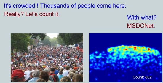
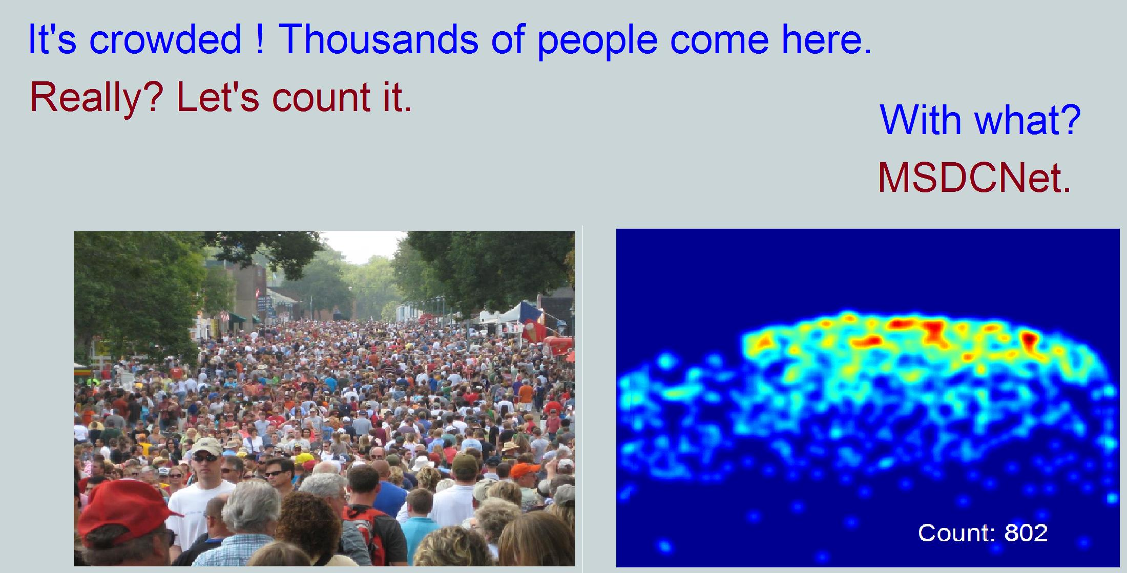
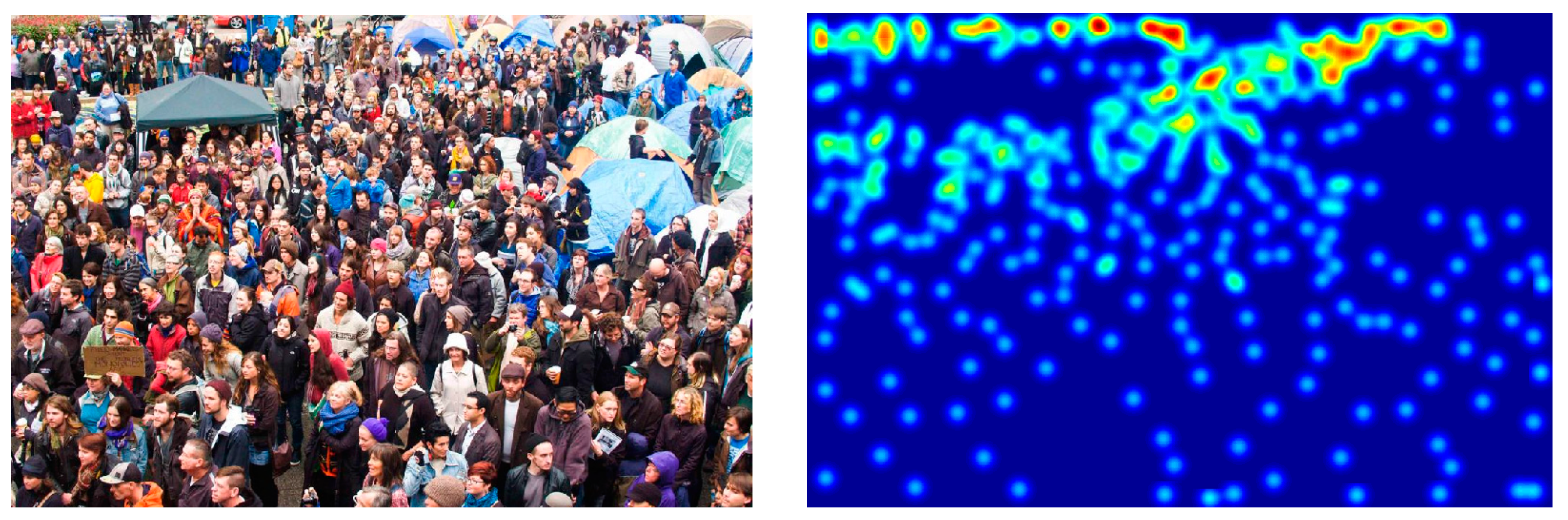
• We propose a multi-scale dilated convolution network (MSDCNet) to estimate the density map of an input crowd image. A multi-scale feature extraction network is designed as the core component of MSDCNet.
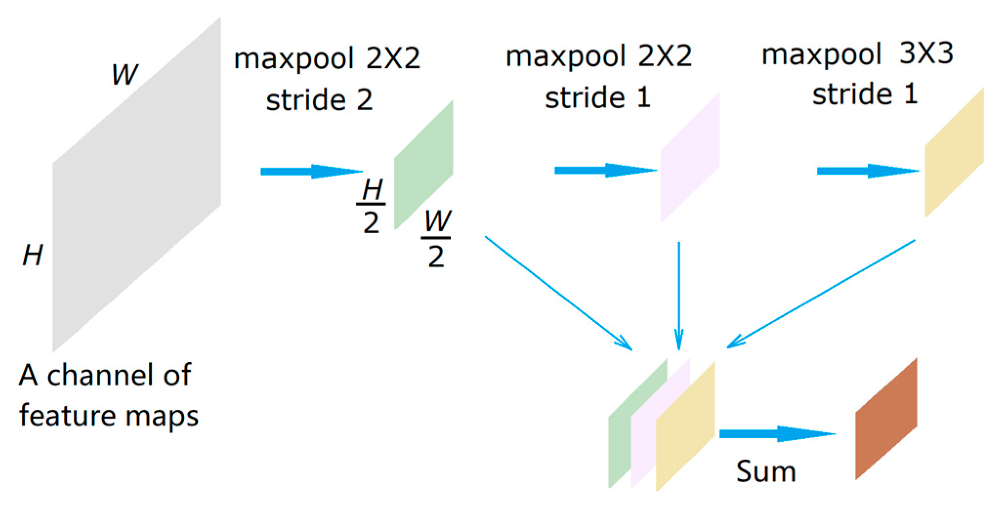
• In the front-end network of MSDCNet, we propose SPP modules to replace max- pooling layers of VGG16 that can extract features with scale invariance. In the back-end network of MSDCNet, we use the dilated convolution layers to replace the traditional alternate convolution and pooling to expand the receptive field, extract high-level semantic information and avoid the loss of spatial information at the same time.
• The effectiveness of our approach is validated on three public datasets, Shanghai_Tech, UCF_CC_50, and UCF_QNRF. Compared with other representative crowd counting models, our model has a better counting performance.

In the rest of this paper, Section 2 includes the recent work related to density estimation. The framework and principle of MSDCNet are described in Section 3. The datasets, experimental results and related analysis are given in Section 4. Conclusions and suggestions for future work are given in Section 5.

2. Related Work

2.1. Density Map

A crowd counting sample generally consists of a crowd image and its label matrix which is the same size as the image. The label matrix stores numbers 0 and 1 that represent the heads’ center-point positions. A visualized label matrix and the corresponding crowd image are shown in Figure 1. The main issue of crowd counting is to find the mapping between input images and density maps through extensive training. The training process of crowd counting models is shown in Figure 2. The preprocessing of training samples includes two objectives: generating ground truth density maps and data augmentation. A sample in datasets provides an image and a set of coordinates of each head-center-point instead of the label matrix mentioned above. The coordinates need to be converted into a label matrix and then into a smooth and continuous density map to serve as the ground truth density map of the training sample (see Section 2.2 for details). Due to the differences in the number of samples, image size, and crowd density among different datasets, the data augmentation for different datasets also varies (see Section 4.1 for details).

2.2. Generating Density Map Based on Gaussian Kernel

First, we initialized a zero matrix with the same size as the input image. Based on the known position coordinates of each head, we set the corresponding elements to 1, and obtained a label matrix composed of 0 and 1. Using the Gaussian kernel and the label matrix for convolution, we obtained a smooth and continuous density map. Due to the variance in the heads’ scale in an image, we adopted an adaptive Gaussian kernel whose size varies with the heads’ scale. After convolution, the 1 at a certain position in the label matrix was replaced with multiple weights between 0 and 1 around it, and the sum of these weights was equal to 1. This not only did not affect the counting of the total number of heads through the density map, but also obtained the spatial information of each head. A ground truth density map obtained via the above method is visualized as a pseudo-color map shown in Figure 3.

2.3. Crowd Counting Models

In 2018, a single-column network, named the congested scene recognition network (CSRNet) [16], was proposed to extract more scale information by using dilated convolutions and expanding the receptive field. CSRNet obtained encouraging counting results in highly congested spaces. In 2020, Jiang et al. [17] proposed trellis encoder–decoder networks (TEDnet) to generate high-quality density estimation maps. They designed multiple decoding columns to hierarchically aggregate spatially endowed features at different encoding stages. Some researchers found out different ways leading to the same target. In order to eliminate the distortion of the crowd image, a reverse perspective network was proposed by Yang et al. [18]. In 2021, a locality-aware crowd counting model was proposed to avoid serious deviation in counting results [19]. A Tencent YouTu team proposed a point-based approach [20]. A set of point proposals is given to represent heads. In [21], an unbalance-based generalized loss function was proposed to improve the training process of the crowd counting model. Introducing an attention mechanism into training is one of the solutions to scale differences in crowd counting [22]. The emergence of various innovative models and learning strategies is continuously improving the accuracy of crowd counting.

3. Proposed Approach

The proposed MSDCNet consists of three parts, a front-end network, a multi-scale feature extraction network (MFENet), and a back-end network, as shown in Figure 4. The crowd-counting task is to obtain the density map instead of classification, so we design it as fully convolutional networks (FCNs). The feature of FCN is that both the input and output are 2D images. The input can be images of any size, while the output size is the same as the input size and they have a corresponding spatial structure. The FCN consists of two parts: a full convolution part (the front-end network and MFENet) which is used to extract features, and a deconvolution part (the back-end network) which is used to obtain the density map estimation by up-sampling.

3.1. Front-end Network

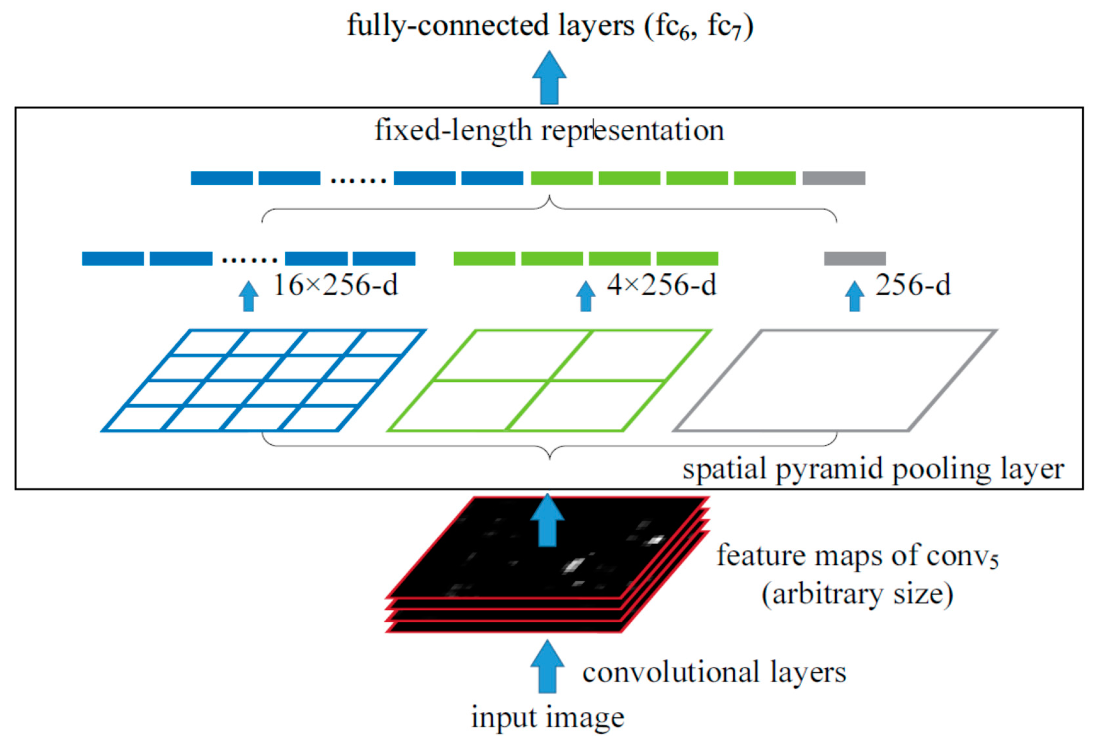
The front-end network is used to extract preliminary features from input images. Because VGG16 [14] performs well in object detection and classification, and has strong transfer learning ability, we used it as the backbone of the front end. VGG16 consists of 13 conv layers, 5 pooling layers, 3 fully connected (FC) layers and a soft-max output layer, as shown in Figure 5. The pooling layer is 2 × 2 max-pooling. After each pooling layer, the width and height of the feature map are reduced by half. With the increase in the network depth, the size of the feature map gradually decreases. The small feature size is not conducive to crowd counting especially in a converged scene. Therefore, to refer to CSRNet [16], the front-end network uses the first 10 conv layers of VGG16 and the 3 pooling layers between them. In order to learn features of multi-scale heads in crowd images, spatial feature fusion is performed in pooling layers in our model. We propose a pooling module based on the SPP idea (denoted as the SPP module) to replace the max-pooling layer.

3.1.1. SPP Module

In 2015, He et al. [23] proposed spatial pyramid pooling (SPP) to address the input size limitation of the standard CNN. As shown in Figure 6, the SPP layer is used after the last conv layer (conv5, with 256 filters) and before the FC layers (fc6, fc7). The SPP extracts the features from the output of conv5 through pooling bins (windows) with different sizes. Each bin obtains one output, so the size of the SPP output features is determined by the number of bins instead of the size of the input. Compared to the breaking fixed size limitation, the most important advantage of the SPP is found by researchers to be that different sizes of bins correspond to different regions of the original image, i.e., to objects of different scales. This greatly improves the robustness of the network to object scaling. The SPP is therefore an effective way to handle multi-scale networks.

Inspired by the different sizes of bins in the SPP, we proposed a SPP module with different pooling kernel sizes to replace the 2 × 2 max pooling layers in VGG16 and to further extract the features with scale invariance. Identical to the original 2 × 2 max-pooling, our SPP module reduces the width and height of the feature map by half, too. Therefore, it is denoted as “SPP-2” in Figure 4. As shown in Figure 7, the SPP module is a stack of three max-pooling layers. The size of the input feature maps is W × H, and the sizes of the three pooling kernels we used are 2 × 2, 2 × 2, and 3 × 3, and the strides are 2, 1, and 1, respectively. Finally, on every channel, the obtained three feature maps of size W/2 × H/2 are summed up. With three SPP modules fusing the spatial features, the front-end network can expand the receptive field and extract features in different scales without increasing the parameters.

3.1.2. Architecture of Front-End Network

The front-end network consists of 10 conv layers and 3 SPP modules, and its architecture is shown in

Table 1. The architecture of the front-end network. The conv layers are denoted as “conv (size)-(number of filters)”. The ReLU activation function is not shown for brevity.

Layers	Kernel	Stride
Conv1	conv3-64	1
Conv2	conv3-64	1
SPP modules	maxpool 2 × 2	2
	maxpool 2 × 2	1
	maxpool 3 × 3	1
Conv3	conv3-128	1
Conv4	conv3-128	1
SPP modules	maxpool 2 × 2	2
	maxpool 2 × 2	1
	maxpool 3 × 3	1
Conv5	conv3-256	1
Conv6	conv3-256	1
Conv7	conv3-256	1
SPP modules	maxpool 2 × 2	2
	maxpool 2 × 2	1
	maxpool 3 × 3	1
Conv8	conv3-512	1
Conv9	conv3-512	1
Conv10	conv3-512	1

. After three SPP modules, the size of the feature map output by the front-end network becomes W/8 × H/8.

3.2. Multi-Scale Feature Extraction Network (MFENet)

In order to perceive the dramatic changes in the scale of the image and extract the multi-scale features of heads, MFENet is designed as the core of MSDCNet in addition to the SPP module in the front-end network.

In order to improve the accuracy of a deep learning model, researchers improve the network structure constantly. The development of a structure design is mainly along two lines; one is the Inception series (i.e., complexity), from GoogLeNet to Inception V2, V3, V4. The other is the VGG series (i.e., depth), which uses a simple structure to make the network as deep as possible, from VGG to ResNet, DenseNet, etc. The core idea of the Inception block is to use parallel sub-networks (conv kernels of different sizes) to achieve perception at different scales, and finally fuse them to obtain better representation of the image. But the complexity of multi-column networks is too great; for example, GoogLeNet consists of 9 Inception blocks and 100+ conv layers. Therefore, we cut off the latter half of VGG16 and replaced it with a multi-column subnet (MFENet) to achieve a balance between complexity and accuracy.

MFENet contains four columns with different perception fields to extract different scales of head features, as shown in

Table 2. The architecture of MFENet. The convolutional layers are denoted as “conv (size)-(number of filters)”. Padding = 1, stride = 1.

Layers	Kernel
Column1	conv1-128
Column2	conv1-128
	conv3-128
Column3	conv1-128
	conv3-128
	conv3-128
Column4	conv1-128
	conv3-128
	conv3-128
	conv3-128

. The first layer of each column is a bottleneck layer, 128 1 × 1 convolutions with a depth of 512. The number of channels of each column is reduced from 512 to 128 due to the bottleneck layer. At the same time, the scale of the feature map extracted by the front-end network is still preserved to cover small targets. One column is only a bottleneck layer and the other columns use stacked 3 × 3 convolutions in one, two, and three layers to implement perceptive fields in sizes of 3 × 3, 5 × 5, and 7 × 7. Thus, MFENet can extract heads’ features in the three scales, large, medium, and small. Multiple small kernels are used consecutively instead of one large kernel, as the latter can significantly reduce the network parameters [14]. For example, to obtain the same 7 × 7 perceptive field, a 7 × 7 kernel has 49 parameters and three 3 × 3 kernels only have 27 parameters. On the other hand, compared to a 7 × 7 conv layer, three 3 × 3 conv layers are two layers deeper and have a stronger ability to fit nonlinearity because the nonlinear activation function ReLU is adopted on each conv layer.

3.3. Back-End Network

The back-end network is designed to expand the receptive field, extract higher-level semantic information, and then conduct up-sampling to obtain a high-quality density map. After the front-end network and MFENet, to achieve these goals we can continue to deepen the network, using alternate conv and pooling layers. However, pooling will further reduce the feature size and decrease the spatial resolution, which is not conducive to obtaining high-quality density maps. Therefore, we use a dilated convolution instead of the combination of conv and pooling to achieve the above goals [16].

A dilated convolution uses sparse kernels to increase the receptive field [24], as shown in Figure 8. In our model, the size of the dilated convolution kernel is 3 × 3. When the dilation rate is 2, the receptive field is expanded to 5 × 5. But the number of parameters is only 9, which is only 36% of that of 5 × 5 standard convolution. Padding is set to 1, so that overfitting can be prevented to avoid the loss of heads’ features while keeping the feature map size unchanged, i.e., without loss of spatial resolution.

Four consecutive dilated convolutional layers are deployed in the back-end network, whose architecture is shown in

Table 3. The architecture of the back-end network. The dilated convolutional layers are denoted as “Dilated conv (size)- (number of filters)”. Padding = 1, stride = 1.

Layers	Kernel	Dilation Rate
Dilated conv1	Dilated conv3-256	1
Dilated conv2	Dilated conv3-128	2
Dilated conv3	Dilated conv3-64	2
Dilated conv4	Dilated conv3-32	2
Conv	conv1-1	-

. After dilated conv layers, a 1 × 1 conv is deployed to output the density map, whose size remains unchanged (W/8 × H/8). In order to obtain a density map of the same size as the input image, up-sampling is conducted by bilinear interpolation to resize the output density map.

3.4. Discussion on Number of Parameters

In order to evaluate the cost of every component of MSDCNet, the number of parameters is calculated without model compression, as shown in

Table 4. The number of parameters in MSDCNet.

Component		Parameters (M)
Front-end network			7.633
MFENet	Column1	65,536	0.360
	Column2	81,920
	Column3	98,304
	Column4	114,688
Back-end network			1.567
Total			9.560

. The total number of parameters is 9.560 M, and the main cost comes from the front-end network, i.e.,the 10 conv layers of VGG16. Three SPP modules are pooling operations without parameters. Due to the bottleneck layers in every column, MFENet only has 0.360 M parameters, about 3.8% of the total number of parameters. Compared to standard convolution with the same kernel size, dilated convolution in the back-end network does not increase the parameters together with the receptive field expanding.

4. Experimental Results and Discussions

The experiments were carried out on a Linux, Ubuntu16.04 operating system, and the model was implemented using the Python 3.8 and PyTorch 1.8.0 library. The experimental environment is an Intel (R) Core (TM) i7-8750H CPU @ 2.60 GHz, DDR4 16 GB memory, and a NVDIA GeForce GTX 1650Ti graphics card.

4.1. Datasets and Data Augmentation

Three public datasets, ShanghaiTech, UCF_CC_50, and UCF-QNRF, were used in our experiments. The statistics of samples and annotations in the datasets are shown in

Table 5. The statistics of samples and annotations in datasets.

Dataset	Number of Samples			Average Resolution		Annotations
	Total	Training Set	Test Set	Training Set	Test Set	Total	Ave	Max
ShanghaiTech_Part_A	482	300	182	872 × 598	861 × 574	241,677	501	3139
ShanghaiTech_Part_B	716	400	316	1024 × 768		88,488	123	578
UCF_CC_50	50	-	-	902 × 653		63,974	1279	4633
UCF-QNRF	1535	1201	334	2896 × 2006	2910 × 2038	1,251,642	815	12,865

. ShanghaiTech includes samples of different scenes and crowd density levels, which are divided into two parts, Part_A and Part_B. The resolution of the images in Part_B is the same. The UCF_CC_50 dataset contains 50 grayscale images with different resolutions and scenes, including sports events, political processions, religious events, etc. The number of people in the images varies significantly, and some images are of extremely dense scenes. The UCF-QNRF dataset contains high-resolution images of outdoor surroundings with green plantation, buildings, streets, the sky and so on. Therefore, UCF-QNRF is of great significance to the dense crowd counting model against background interference.

In ShanghaiTech and UCF-QNRF, samples were divided into a training set and a test set, but the size of three training sets was not large enough. The training sets and UCF_CC_50 were expanded. In order to compare them with other counting models under the same conditions, we used the general data enhancement method [16]. Nine patches of 1/4 size were cropped from an original image; four of them were nonoverlapping areas (top left, bottom left, top right, and bottom right), and the other five patches were randomly cropped. All patches and the original image were then mirrored. Finally, the sample size was expanded to 20 times the original ones. After expansion, UCF_ CC_ 50 contained only 1000 samples, so we randomly cropped the very dense and high-resolution samples to expand the dataset to 7500 samples in total. A fivefold cross-validation was conducted, in which 6000 images were used for training and 1500 images were used for testing.

4.2. Evaluation Metrics

We used the commonly used measures of crowd counting [25], the mean absolute error (MAE) and mean squared error (MSE), which are defined as follows:

$$MAE=\frac{1}{N}{\displaystyle \sum _{i=1}^N\left|C_i-{\widehat{C}}_i\right|},MSE=\sqrt{\frac{1}{N}{\displaystyle \sum _{i=1}^N{\left|C_i-{\widehat{C}}_i\right|}^2}}$$

(1)

where N is the number of input images, $C_i$ is the actual number of people in the i th image, and ${\widehat{C}}_i$ is the estimated number of people in the i th image. The lower the MAE is, the higher is counting accuracy; the lower the MSE is, the better the network’s robustness is.

4.3. Network Training

The MSDCNet consists of three parts, and we train them separately from easy to difficult as follows:

• Training the back-end network. The dimensions of MFENet’s input and output are same (H/8 × W/8 × 512), so we can remove it first and connect the back end to the front end directly. The front-end network adopts VGG16’s pretrained model on ImageNet. We then freeze the front end and set the back end to trainable. We then obtain a preliminary back end.
• Fine-tuning the front-end network. We freeze the back end, and train the front end from the pretrained weights of VGG16.
• Training MFENet column to column. We put MFENet back into our model. At first, we froze the front end, back end, and column 2, 3, and 4 of MFENet, and only set column1 to trainable. After column1 was trained, we trained column 2 starting at part of the weights coming from column1. After four columns had been trained one by one, we trained them together.
• Fine-tuning the model in order from back end to front end and then to MFENet.

Our model was trained using the Adam optimizer, the ReLU activation function and the Euclidean distance loss. The initial learning rate was set to 0.002 with a decay factor of 0.005 and a momentum value of 0.9.

4.4. Experimental Results on the ShanghaiTech Dataset

After data augmentation, the training set of ShanghaiTech Part_A and Part_ B were expanded to 6000 and 8000 images. Some density maps generated by MSDCNet are shown in Figure 9. The comparison of the counting errors between MSDCNet and other models is shown in

Table 6. Counting errors on ShanghaiTech dataset.

Method	Part_A			Part_B
	MAE↓	MSE	Parameters (M)	MACs (G)	MAE	MSE	MACs (G)
MCNN [15]	110.2	173.2	0.133	13.989	26.4	41.3	21.097
SwitchCNN [26]	90.4	135.0	15.108	164.182	21.6	33.4	247.610
MSCNN [27]	83.8	127.4	3.084	288.706	17.7	30.2	435.412
CP-CNN [28]	73.6	106.4	17.137	254.311	20.1	30.1	383.537
CSRNet [16]	68.2	115.0	16.259	215.405	10.6	16.0	324.862
SANet [29]	67.0	104.5	1.146	49.334	8.4	13.6	74.403
TEDNet [17]	64.2	109.1	8.863	367.193	8.2	12.8	553.780
DUBNet [30]	64.6	106.8	18.827	52.172	7.7	12.5	78.683
MSDCNet (Ours)	60.9	97.2	9.560	160.804	6.9	11.2	242.516

. Besides the accuracy, the parameters and time complexity of every model are compared, too. The time complexity is related to the size of the input image; here, we use the average resolution of training set samples (as shown in Table 5). Only the multiply-accumulate operations (MACs) of conv and FC layers were considered; pooling, BN and ReLU were conventionally ignored.

The experimental results show that our model achieves the best counting accuracy. On the Part_A dataset, the MAE of MSDCNet decreased by 3.7 and the MSE decreased by 9.6 compared to the best-performing model, DUBNet. On the Part_B dataset, the MAE decreased by 0.8 and the MSE decreased by 1.3. The backbone of DUBNet is ResNet50 and its MACs are much lower than ours because a large number of residual blocks is used. This also leads to its parameters being almost twice the size of ours. From the perspective of model volume, the MCNN has the lowest parameters and time complexity. Due to the stacked nine multi-scale encoders with a four-column structure, TEDNet has significant MACs. TEDNet used nine multi-scale encoders with multi-column structures, resulting in a significant increase in the model complexity. Compared with SwitchCNN whose MACs are similar to ours, our parameters were 37% less and the accuracy was greatly improved.

4.5. Experimental Results on the UCF_CC_50 Dataset

The fivefold cross-validation result of our model on the UCF_CC_50 dataset is shown in Figure 10. Some density maps generated by MSDCNet are shown in Figure 11. The comparison of the counting errors between MSDCNet and other models on the UCF_CC_50 dataset is shown in

Table 7. Counting errors on UCF_CC_50 dataset.

Method	MAE↓	MSE	Parameters (M)	MACs (G)
MCNN [15]	377.6	509.1	0.133	15.801
MSCNN [27]	363.7	468.4	3.084	326.106
SwitchCNN [26]	318.1	439.2	15.108	185.450
CP-CNN [28]	295.8	320.9	17.137	287.254
CSRNet [16]	266.1	397.5	16.259	243.308
SANet [29]	258.4	334.9	1.146	55.725
DUBNet [30]	243.8	329.3	18.827	58.930
MSDCNet (ours)	206.9	271.3	9.560	181.635

. The experimental results show that our model achieves excellent counting accuracy on UCF_CC_50. The MAE of MSDCNet decreased by 36.9 and the MSE decreased by 58.0 compared to the DUBNet with the best performance. The average crowd number of samples in UCF_CC_50 was 1279, which is much larger than that of other datasets. Therefore, it can be seen that our model performs well in extremely dense crowds. MSCNN has only about three M parameters because of its concise structure, but has the maximum MACs because it has fewer pooling layers. In our model, both complexity and parameters are taken into account. There are three pooling modules in the front end, so that the subsequent computation can be controlled in a reasonable range.

4.6. Experimental Results on the UCF-QNRF Dataset

The UCF-QNRF dataset contains dense crowd images with multiple scenes, views, and illuminations, and is important for verifying the robustness of counting models. Some density maps generated by MSDCNet from the UCF-QNRF dataset are shown in Figure 12. The comparison of the counting errors between MSDCNet and other models on the UCF-QNRF dataset is shown in

Table 8. Counting errors on the UCF-QNRF dataset.

Method	MAE↓	MSE	Parameters (M)	MACs (G)
SwitchCNN [26]	228	445	15.108	1829.095
RAZ-Net [31]	116	195	24.465	4848.993
TEDNet [17]	113	188	8.863	4090.777
DUBNet [30]	105.6	180.5	18.827	581.231
MSDCNet (ours)	101.4	170.9	9.560	1791.465

. The experimental results show that our model achieves better counting accuracy on UCF-QNRF than other models. The MAE of MSDCNet decreased by 4.2 and the MSE decreased by 9.6 compared to DUBNet with the best performance. And MSDCNet shows excellent robustness on the UCF-QNRF dataset.

4.7. Ablation Experiments

To verify the effectiveness of the proposed MFENet, the SPP module and dilated conv layers, three ablation experiments were conducted. In the first experiment, MFENet in MSDCNet was removed and the model only consisted of a front-end and back-end network. It is denoted as model-A, as shown in Figure 13a. In the second experiment, MFENet was preserved, three SPP modules in the front end were removed, and the original 2 × 2 max-pooling layers in VGG16 were used. This is denoted as model-B, as shown in Figure 13b. In the third experiment, four dilated conv layers of the back end were replaced with four standard conv layers and a pooling layer. This is denoted as model-C, as shown in Figure 13c. The models are trained and tested on the UCF-QNRF dataset and the experimental results are shown in

Table 9. Ablation experimental results on UCF-QNRF dataset.

Model	MAE	MSE
model-A (MSDCNet without MFENet)	185.6	268.1
model-B (MSDCNet without SPP module)	163.3	238.7
model-C (MSDCNet without dilated conv)	117.1	185.5
MSDCNet	101.4	170.9

.

The experimental results indicate that:

• From the counting errors of the two experimental models and MSDCNet, it can be seen that after removing MFENet and the SPP, the counting accuracy of MSDCNet significantly decreased. Without MFENet, the MAE of model-A increased by 84.2 (about 45% of model-A’s MAE), and the MSE increased by 97.2 (about 36% of model-A’s MSE). Without the SPP module, the MAE of model-B increased by 61.9 (about 38% of the MAE of model-B), and the MSE increased by 67.8 (about 28% of the MSE of model-B). Without dilated conv layers, the MAE of model-C increased by 15.7 (about 13% of the MAE of model-C), and the MSE increased by 14.6 (about 8% of the MSE of model-C). These fully demonstrate the effectiveness of MFENet, the SPP modules and the dilated conv layers in our model.
• From the counting errors of the three experimental models, it can be seen that the counting error of model-A is higher than that of model-B and model-C, indicating that MFENet makes a greater contribution to the counting accuracy of the entire network than the SPP modules and dilated conv layers.

5. Conclusions

The proposed crowd counting model solved the problems of uneven crowd distribution and variance of heads scale, achieved high counting accuracy and good robustness on three public datasets. The one-column framework of the backbone simplified the model’s structure and kept a certain depth to extract high-level features. The proposed SPP modules in the front end fused the spatial features in pooling and helped the front end to extract features in a different scale without increasing the parameters. By connecting a multi-column subnet (MEFNet) to the one-column backbone, we achieved a compromise result between precision and complexity. Only by increasing the parameters by 3.8% did MEFNet perceive the dramatic changes in the scale of the image and extract the multi-scale features of the heads. The consecutive dilated convolution layers used as the back end prevented overfitting effectively to avoid the loss of head features, expanded the receptive field, and improved the quality of the output density maps.

In future research, we will investigate the impact of the background and image edge, and establish a dense crowd counting model with higher accuracy and better robustness.

References

1. Zhang, J.; Liu, J.; Wang, Z. Convolutional Neural Network for Crowd Counting on Metro Platforms. Symmetry 2021, 13, 703. [Google Scholar] [CrossRef]
2. de Silva, E.M.K.; Kumarasinghe, P.; Indrajith, K.K.D.A.K.; Pushpakumara, T.V.; Vimukthi, R.D.Y.; de Zoysa, K.; Gunawardana, K.; de Silva, S. Feasibility of using convolutional neural networks for individual-identification of wild Asian elephants. Mamm. Biol. 2022, 102, 931–941. [Google Scholar] [CrossRef]
3. Lu, W.G.; Tan, Z. Research on Crowded Trampling Accident Prevention and Disposal in Urban Public Places: The Case of Itaewon Trampling Accident in Korea. China Emerg. Rescue 2023, 1, 4–10. [Google Scholar]
4. Gao, G.; Gao, J.; Liu, Q.; Wang, Q.; Wang, Y. CNN-based Density Estimation and Crowd Counting: A Survey. In Proceedings of the IEEE Conference on Computer Vision and Pattern Recognition (CVPR), Seattle, WA, USA, 14–19 June 2020. [Google Scholar]
5. Zhao, R.; Dong, D.; Wang, Y.; Li, C.; Ma, Y.; Enriquez, V.F. Image-Based Crowd Stability Analysis Using Improved Multi-Column Convolutional Neural Network. IEEE Trans. Intell. Transp. Syst. 2021, 23, 5480–5489. [Google Scholar] [CrossRef]
6. Chan, A.B.; Liang, Z.S.; Vasconcelos, N. Privacy preserving crowd monitoring: Counting people without people models or tracking. In Proceedings of the 2008 IEEE Conference on Computer Vision and Pattern Recognition (CVPR), Anchorage, AK, USA, 23–28 June 2008. [Google Scholar]
7. Chan, A.B.; Vasconcelos, N. Bayesian Poisson regression for crowd counting. In Proceedings of the IEEE Conference on Computer Vision and Pattern Recognition (CVPR), San Francisco, CA, USA, 6 May 2010. [Google Scholar]
8. Wan, H.L.; Wang, X.M.; Peng, Z.W.; Bai, Z.; Yang, X.; Sun, J. A dense crowd counting algorithm based on a novel multi-scale attention mechanism. J. Electron. Imaging 2022, 44, 1129–1136. [Google Scholar]
9. Jiang, N.; Zhou, O.; Yu, F.H. A review of computer vision-based target counting methods. Laser Optoelectron. Prog. 2021, 58, 43–59. [Google Scholar]
10. Meng, Y.B.; Chen, X.R.; Liu, G.H.; Xu, S.J. Crowd density estimation method based on multi-feature information fusion. Laser Optoelectron. Prog. 2021, 58, 276–287. [Google Scholar]
11. Wang, Y.; Zhang, W.; Huang, D.; Liu, Y.; Zhu, J. Multi-scale features fused network with multi-level supervised path for crowd counting. Expert Syst. Appl. 2022, 59, 200–212. [Google Scholar] [CrossRef]
12. Krizhevsky, A.; Sutskever, I.; Hinton, G.E. ImageNet Classification with Deep Convolutional Neural Networks. In Proceedings of the Neural Information Processing Systems (NIPS), Lake Tahoe, NV, USA, 3–8 December 2012. [Google Scholar]
13. Szegedy, C.; Liu, W.; Jia, Y.; Sermanet, P.; Reed, S.; Anguelov, D.; Erhan, D.; Vanhoucke, V.; Rabinovich, A. Going Deeper with Convolutions. In Proceedings of the IEEE Conference on Computer Vision and Pattern Recognition (CVPR), Columbus, OH, USA, 23–28 June 2014. [Google Scholar]
14. Simonyan, K.; Zisserman, A. Very deep convolutional networks for large-scale image recognition. In Proceedings of the IEEE Conference on Computer Vision and Pattern Recognition (CVPR), Boston, MA, USA, 7–12 June 2015. [Google Scholar]
15. Zhang, Y.; Zhou, D.; Chen, S.; Gao, S.; Ma, Y. Single-image crowd counting via multi-column convolutional neural network. In Proceedings of the IEEE Conference on Computer Vision and Pattern Recognition (CVPR), Las Vegas, NV, USA, 26 June-1 July 2016. [Google Scholar]
16. Li, Y.; Zhang, X.; Chen, D. CSRNet: Dilated Convolutional Neural Networks for Understanding the Highly Congested Scenes. In Proceedings of the 2018 IEEE/CVF Conference on Computer Vision and Pattern Recognition, Salt Lake City, UT, USA, 18–23 June 2018; pp. 1091–1100. [Google Scholar]
17. Jiang, X.L.; Xiao, Z.H.; Zhang, B.C.; Zhen, X.; Cao, X.; Doermann, D.; Shao, L. Crowd counting and density estimation by trellis encoder-decoder networks. In Proceedings of the IEEE Conference on Computer Vision and Pattern Recognition (CVPR), Seattle, WA, USA, 14–19 June 2020. [Google Scholar]
18. Yang, Y.; Li, G.; Wu, Z.; Su, L.; Huang, Q.; Sebe, N. Reverse Perspective Network for Perspective-Aware Object Counting. In Proceedings of the IEEE Conference on Computer Vision and Pattern Recognition (CVPR), Seattle, WA, USA, 14–19 June 2020. [Google Scholar]
19. Zhou, J.T.; Zhang, L.; Du, J.; Peng, X.; Fang, Z.; Xiao, Z.; Zhu, H. Locality-Aware Crowd Counting. IEEE Trans. Pattern Anal. Mach. Intell. 2022, 44, 3602–3613. [Google Scholar] [CrossRef] [PubMed]
20. Song, Q.; Wang, C.; Jiang, Z.; Wang, Y.; Tai, Y.; Wang, C.; Li, J.; Huang, F.; Wu, Y. Rethinking Counting and Localization in Crowds: A Purely Point-Based Framework. In Proceedings of the IEEE International Conference on Computer Vision (ICCV), Montreal, QC, Canada, 10–17 October 2021. [Google Scholar]
21. Wan, J.; Liu, Z.; Chan, A.B. A Generalized Loss Function for Crowd Counting and Localization. In Proceedings of the Computer Vision and Pattern Recognition, Online; 2021. [Google Scholar]
22. Lin, H.; Ma, Z.H.; Ji, R.R. Boosting Crowd Counting via Multifaceted Attention. In Proceedings of the IEEE Conference on Computer Vision and Pattern Recognition (CVPR), New Orleans, LA, USA, 19–24 June 2022. [Google Scholar]
23. He, K.; Zhang, X.; Ren, S.; Sun, J. Spatial Pyramid Pooling in Deep Convolutional Networks for Visual Recognition. IEEE Trans. Pattern Anal. Mach. Intell. 2015, 37, 1904–1916. [Google Scholar] [CrossRef] [PubMed] [Green Version]
24. 24. Fisher, Y.; Koltun, V. Muti-scale context aggregation by dilated convolutions. In Proceedings of the International Conference on Learning Representations (ICLR), San Juan, Puerto Rico, 2–5 May 2016. [Google Scholar]
25. Liu, W.; Salzmann, M.; Fua, P. Context-aware crowd counting. In Proceedings of the IEEE Conference Computer Vision and Pattern Recognition (CVPR), Long Beach, CA, USA, 16–20 June 2019. [Google Scholar]
26. Sam, D.B.; Surya, S.; Babu, R.V. Switching convolutional neural network for crowd counting. In Proceedings of the 2017 IEEE Conference on Computer Vision and Pattern Recognition (CVPR), Honolulu, HI, USA, 21–26 July 2017. [Google Scholar]
27. Zeng, L.; Xu, X.; Cai, B.; Qiu, S.; Zhang, T. Multi-scale convolutional neural networks for crowd counting. In Proceedings of the IEEE International Conference on Image Proceeding (ICIP), Beijing, China, 17–20 September 2017. [Google Scholar]
28. Sindagi, V.A.; Patel, V.M. Generating high-quality crowd density maps using contextual pyramid CNNs. In Proceedings of the IEEE International Conference on Computer Vision (ICCV), Venice, Italy, 22–29 October 2017. [Google Scholar]
29. Cao, X.; Wang, Z.; Zhao, Y.; Su, F. Scale Aggregation Network for Accurate and Efficient Crowd Counting. In Proceedings of the European Conference on Computer Vision (ECCV), Munich, Germany, 8–14 September 2018. [Google Scholar]
30. Oh, M.H.; Olsen, P.; Ramamurthy, K.N. Crowd Counting with Decomposed Uncertainty. In Proceedings of the AAAI Conference on Artificial Intelligence, New York, NY, USA, 7–12 February 2020. [Google Scholar]
31. Liu, C.; Weng, X.; Mu, Y. Recurrent Attentive Zooming for Joint Crowd Counting and Precise Localization. In Proceedings of the IEEE Conference on Computer Vision and Pattern Recognition (CVPR), Long Beach, CA, USA, 16–20 June 2019. [Google Scholar]
Figure 1. Visualization of a label matrix.
Electronics 12 02624 g001
Figure 2. The training diagram of crowd counting models.
Electronics 12 02624 g002
Figure 3. Generated Gaussian kernel density map by adaptive Gaussian kernel convolution.
Electronics 12 02624 g003
Figure 4. The framework of the MSDCNet. The convolution layers are denoted as “conv (size)(number of filters)”, the dilated convolution layers are denoted as “Dilated conv (size)-(number of filters), dilation rate”.
Electronics 12 02624 g004
Figure 5. The framework of VGG16.
Electronics 12 02624 g005
Figure 6. The network structure with a SPP layer.
Electronics 12 02624 g006
Figure 7. The framework of the proposed SPP module.
Electronics 12 02624 g007
Figure 8. Dilated convolution. The kernel size is 3 × 3, dilation rate = 2.
Electronics 12 02624 g008
Figure 9. Some density maps generated by MSDCNet from ShanghaiTech dataset. The ground truth density maps are shown in the medium column, and the estimated ones are shown in the right column.
Electronics 12 02624 g009aElectronics 12 02624 g009b
Figure 10. Bar chart of counting errors of the fivefold cross-validation.
Electronics 12 02624 g010
Figure 11. Density maps on UCF_CC_50 test set. The ground truth density maps are shown in the medium column and the estimated ones are shown in the right column.
Electronics 12 02624 g011
Figure 12. Some density maps generated by MSDCNet from the UCF-QNRF test dataset.
Electronics 12 02624 g012
Figure 13. The frameworks of models in ablation experiments. (a) model-A: model w/o MFENet; (b) model-B: model w/o SPP modules; (c) model-C: model w/o dilated conv.
Electronics 12 02624 g013