X-ray Security Inspection Image Dangerous Goods Detection Algorithm Based on Improved YOLOv4

Abstract

Aiming at the problems of multi-scale and serious overlap of dangerous goods in X-ray security-inspection-image samples, an X-ray dangerous-goods-detection algorithm with high detection accuracy is designed based on the improvement of YOLOv4. Using deformable convolution to redesign YOLOv4’s path-aggregation-network (PANet) module, deformable convolution can flexibly change its receptive field based on the shape of the detected object. When the high-level information and low-level information are fused in the PANet module, deformable convolution is used to align features, which can effectively improve the detection accuracy. Then, the Focal-EIOU loss function is introduced, which can solve the problem of the CIOU loss function being prone to causing severe loss-value oscillation when dealing with low-quality samples. During training, the network can converge more quickly and the detection accuracy can be slightly improved. Finally, Soft-NMS was used to improve the non-maximum suppression of YOLOv4, effectively solving the problem of the high overlap rate of hazardous materials in the X-ray security-inspection dataset and improving accuracy. On the SIXRay dataset, this model detected 95.73%, 83.00%, 82.95%, 85.13%, and 80.74% AP for guns, knives, wrenches, pliers, and scissors, respectively, and the detected mAP reached 85.51%. The proposed model can effectively reduce the false-detection rate of dangerous goods in X-ray security images and improve the detection ability of small targets.

1. Introduction

X-rays can penetrate substances and interact with them to produce high-resolution images with rich internal details, which is conducive to the detection of high-density contraband hidden inside objects [1]. Different materials have different degrees of X-ray absorption and scattering attenuation, and the corresponding X-ray images generated by the goods have different colors. Because of the advantages of using X-ray to detect dangerous goods in baggage, such as the little damage to goods, non-necessity of unpacking, its safety and reliability, and its easy operation, it is widely used in various places requiring security inspection.

At present, the X-ray safety inspection for dangerous goods is still manual monitoring. The security inspector needs to observe the X-ray-scanned image on the screen with the naked eye and judge whether there are dangerous goods based on their own experience. The accuracy of the inspection of prohibited goods depends on the proficiency and mental state of the security inspector. In addition, there are many uncertainties in the number of items in the X-ray security-inspection images, and not all luggage contains dangerous items, which greatly affects the alertness of security inspectors while increasing the difficulty of detection, resulting in an increase in the rate of missed detection.

Compared with natural images, X-ray images are characterized by low contrast, limited color range, poor texture, and serious overlap [2]. Therefore, experts have conducted deep research on the characteristics of designing, labeling, and selecting X-ray-image data. Bastan et al. compared the performance of various feature detectors and a combination of different descriptors, proving the feasibility and potential of traditional methods of manual features in X-ray-image detection [3]. Mikolaj et al. found that the methods of a visual word bag yielded great differences in terms of the feature detector, feature descriptor, word size, and final classification method, and further proved that the use of feature-point density as a simple measure of image complexity is a component of the overall classifier [4].

In 2017, Mery et al. proposed separating the target and background of an X-ray image using the adaptive sparse-representation method to improve the performance of the detection of dangerous goods [5]. In 2018, Xing Xiaolan et al. used the method of median filtering to de-noise X-ray security images and used two gray-projection algorithms to find the area with the smallest gray value in the image to carry out the detection of the X-ray security image [6]. Russo et al. used the approximate-median-filter algorithm to remove the background from the input image and then used the shape-based-filtering method to obtain the region of interest, calculated the local binary pattern (LBP) and histogram based on the pixels of the region of interest to form the feature vector, and finally used a support vector machine (SVM) to classify [7]. In 2019, Santos et al. implemented bilateral filtering-preprocessing technology before the detection phase to improve the accuracy and used color-threshold processing and Hough transform in the HSV color space to effectively segment the region of interest. In the detection phase, the directional-gradient histogram was extracted from the image as the key feature of classification [8]. Li Hai et al. used X-ray images for bilateral filtering processing to select an image with rich edge information, and each channel was subject to homomorphic filtering processing, which could effectively assist with the detection of dangerous goods in X-ray images [9].

Although the method of detecting dangerous goods based on traditional X-ray security images has strong interpretability, the efficiency of manual feature extraction is low, and the performance of traditional methods in processing large amounts of data and rapid detection is not ideal.

Due to the significant improvement in the parallel-computing ability of computer systems and the emergence of a large number of X-ray security-image data, the X-ray security-image technology for detecting dangerous goods based on the deep-learning method has gradually become the preferred method of most researchers, as it can realize automatic extraction of multiple features of the image [10], thus avoiding the traditional image-feature-extraction operation, and has good invariance features, such as displacement and scaling, as well as good scalability, which are great advantages in X-ray security-image detection [11].

In 2017, Akcay et al. used transfer learning to conduct pre-training on an ImageNet dataset with Faster RCNN, and the mAP reached 88.3% [12]. Zhu et al. improved the Faster RCNN detection model through appropriate anchor selection and the non-maximum-suppression (NMS) algorithm, and achieved excellent detection performance [13]. In 2018, Singh et al. proposed the R-FCN300 model to improve the detection speed by solving the problem of repeated calculation of ROI in Fast RCNN and decoupling the classification branch [14]. Zhang et al. improved on the basis of the SDD network, proposed the Detection with Enriched Semantics (DES) model, used the segmentation module to increase the semantic information of low-level feature maps, and used the global-activation module to enhance the semantic information of high-level feature maps [15].

In 2019, Guo et al. used ResNet101 to replace the backbone network of the basic network SSD to obtain stronger anti-degradation performance to build the SSD-Resnet101 structure. On this basis, the shallow features are used to fuse with the deep features to increase the receptive field of the shallow-feature map. Full use is made of context information to improve the detection accuracy of small and medium-sized target dangerous goods in safety inspections [16]. In order to explore the transferability brought by different shapes, different image resolutions, and different colors in X-ray images, Gaus et al. used the transfer-learning method to evaluate the network structures of Faster R-CNN, Mask R-CNN, and RetinaNet, among which Faster R-CNN had the best detection performance [17].

In 2020, Tang Haoyang et al. used deformable convolution to reconstruct the feature-pyramid structure of the SSD network to improve the detection accuracy of the network in order to extract the deeper semantic features of dangerous goods when the feature pyramid is fused [18]. Yu et al. proposed an SSD-X detection network. Considering the position uncertainty and overlap of the target, multiple data enhancement is used to effectively improve the accuracy and over-fitting phenomenon. The focus loss is introduced into the confidence-loss function to accelerate the convergence rate of the model [19].

In 2021, Guo Shouxiang et al. believed that the composite-backbone-network structure has a stronger ability to extract features. On the basis of YOLOv3, the composite-backbone network was used to build the YOLO-C network to improve the detection accuracy of the network [20]. On the basis of CenterNet, Tang et al. used ResNet-50 to improve its backbone network to improve detection speed and added a sampling layer to the feature-processing network to improve detection accuracy [21].

In 2022, Kumar et al. proposed a multi-channel region-recommendation network (MCRPN) to solve the scale difference of dangerous goods in X-ray-image recognition and achieve a faster RCNN network, which uses different levels of convolution features in visual semantics and integrates the richer semantic information at the upper level of VGG16 and the shallower edge features at the lower level to map the multi-scale candidate-target area to the corresponding feature map [22]. Jiang et al. proposed the AM-YOLO model, adding the SE-attention module to the backbone network of YOLOv4 to distinguish the importance of feature-map channels, and proposed a new path-aggregation network to achieve the fusion of shallow and deep features, thus improving the network model-detection ability [23].

We proposed a combination of deformable convolution and the path-aggregation-network (PANet) module of the YOLOv4 network, and designed and implemented a dangerous-goods-detection algorithm for X-ray security-inspection images. The main contribution of the proposed method is summarized as follows:

1. This paper proposes combining deformable convolution with the PANet module of the YOLOv4 network and using the more flexible receptive field of deformable convolution to solve the problem of feature misalignment in the feature-fusion module of YOLOv4 in the process of high- and low-level feature fusion.

2. Based on the backbone network, a channel-pruning algorithm is designed to remove redundant channels in the network, reduce the amount of computation, and improve the reasoning speed of the network model. Experiments show that this method can effectively improve the inference speed of network models and meet the requirements of real-time security checks in terms of speed.

2. Related Work

X-ray security-inspection images mainly have the following characteristics:

(1) Serious loss of detail and color features: Due to the X-ray-imaging method and the material of the object itself, the original color information and detailed information on the contour of the object are lost during imaging.

(2) Background interference: When the background material is the same as the object, contour information similar to the object color is generated, which interferes with the model’s learning of object-feature information during training.

(3) Serious-overlap phenomenon: The shape of an object undergoes significant changes under ray projection, and the random placement of positions and the overlapping placement of multiple objects results in complex, overlapping, and occluding contours of the object formed by X-rays passing through the object, increasing the difficulty of extracting effective features of various categories.

(4) The scale of prohibited items is diverse: Even within a single X-ray security image, the size of prohibited items is diverse, and the same object may even exhibit different sizes due to issues such as angle, compression, and image size.

Based on the characteristics of X-ray images, Mery et al. [11] evaluated 10 X-ray contraband-detection methods based on visual-pool-bag models, sparse representations, deep learning, and classical pattern-recognition schemes, and found that deep-learning methods performed the best. Miao et al. [24] proposed a class-balance hierarchical-refinement model that uses different scale features to filter irrelevant information and identify and classify prohibited items. Wei et al. [25] proposed a deblocking attention module that utilizes edge information and material information of prohibited items to generate attention maps and feature maps for detection. Gu et al. [26] proposed using feature-enhancement modules to improve feature-extraction capabilities while utilizing multi-scale fusion to obtain more accurate regions of interest, improving the accuracy and robustness of prohibited-item detection in X-ray security images.

The above methods have greatly improved the detection accuracy and laid the foundation for the development of X-ray-security prohibited-item detection. However, in real scenes, the variable shape and scale of targets, severe overlapping occlusion, and complex background interference are still key issues that need to be addressed in current research, especially the challenges brought on by the characteristics of X-ray-security images of prohibited items themselves. The current detection accuracy still does not meet the requirements of practical applications. On the one hand, the scale and shape of contraband vary greatly, the distribution of context information is uneven, and conventional convolution cannot adapt to the receptive field of the actual target and cannot flexibly handle the height change of context distribution due to its fixed sampling location, which ultimately causes some important context information to be ignored, weakening the ability of feature extraction. On the other hand, items of the same material present the same or similar colors in the image, which can easily cause confusion between the target and the background when overlapping and obstructing, and can even not be distinguished. When these items are processed through convolutional layers, they receive similar feature responses, resulting in a decrease in recognition and positioning accuracy.

3. Improved YOLOv4 Model

The YOLO network is a target-detection network based on regression. It can complete classification and location tasks of targets in a network directly and simultaneously by fully extracting the features of the detected targets, and truly realizes a simple and efficient end-to-end design idea. The YOLOv4 algorithm has a more complex network structure but has higher accuracy and faster speed, and shows a significant improvement in detecting small targets and occluded targets.

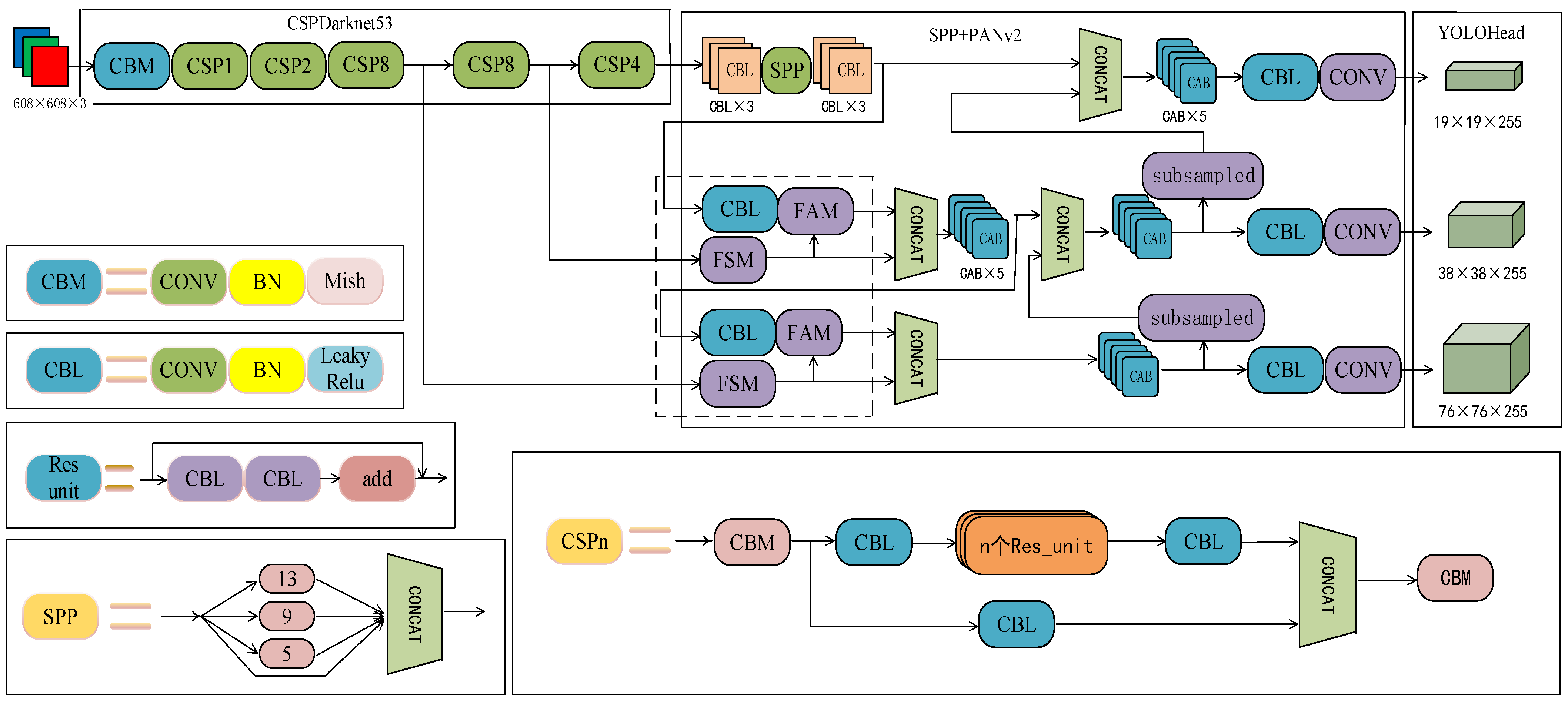
There will be many targets of different sizes in the X-ray-detection task, and different targets have different characteristics, resulting in a low accuracy rate of judgment only through target characterization when detecting dangerous goods. YOLOv4’s neck adopts the PAN structure for fusion, uses shallow features to distinguish simple targets, uses deep features to distinguish complex targets, transfers high-level strong semantic features, enhances the whole pyramid, enhances semantic information, adds a bottom-up pyramid, transfers low-level location features, combines semantic information, and has location information. However, PAN ignores the problem of feature alignment. The direct splicing between up-sampling and local features cause the feature map to have an unaligned context, which turns into errors in prediction, especially on the object boundary.

This improved design proposes a feature-selection module that can adaptively learn the bottom-up feature map containing more spatial details to achieve accurate positioning. A feature-alignment module is proposed that aligns the up-sampling feature with a set of reference features by adjusting each sampling position in the convolution kernel using the learned offset. The two modules are integrated into the PAN structure, and the PANv2 structure is proposed as shown in Figure 1.

3.1. The Deformable Convolution

The neck of YOLOv4 uses the PANet module to fuse the high- and low-level features and combines the semantic information and location information. However, the direct splicing between the upper sampling and local features may cause the feature map to contain misaligned context information, which can be converted into errors in prediction, especially on the object boundary, resulting in poor accuracy when detecting dangerous goods. Deformable convolution [27] introduces offset in the receptive field, which is different from the square receptive field of traditional convolution. This feature can be used to achieve more accurate feature alignment and improve the accuracy of detection.

The standard convolution layer usually uses sliding-window and scale-invariant feature transformation to deal with the geometric changes of the object. It can effectively expand the receptive field by stacking more convolution layers, but the corresponding calculation cost increases exponentially with the increase of the receptive field. With the increase in depth, the receptive field goes far beyond the area of interest, resulting in the extracted features being affected by redundant context information. The deformable convolution can adaptively determine the size of the receptive field and flexibly adjust the receptive field by learning the additional offset of the convolution network.

Traditional convolution uses a regular grid as the convolution kernel, slides on the input-characteristic graph step by step, and calculates the point product sum of the matrix of the input characteristic graph one by one, and finally adds the variation. The size of the convolution kernel determines the size of the receptive field. The corresponding value of each position in the output-characteristic diagram is calculated as shown in Formula (1):

$${\mathrm{y}(\mathrm{p}}_0)={\displaystyle \sum _{{\mathrm{p}}_n\in R}w({\mathrm{p}}_n)}·x({\mathrm{p}}_0{+\mathrm{p}}_n)$$

(1)

where $y$ represents the output-feature map, $x$ represents the input-feature map, $w$ represents the weight coefficient, $b$ represents the deviation, ${\mathrm{p}}_0$ is the 0th point in the grid, and ${\mathrm{p}}_n$ is the nth point in the grid.

The deformable convolution adds a learnable offset parameter on the basis of ordinary convolution, which can be used to adjust the receptive field to better extract the features of complex-shaped objects. In the deformable convolution, $\{\Delta p_n|n=1,\cdots ,N\}$ is considered an offset. The offsets of each position are enumerated on the convolutional kernel when $N=\left|R\right|$, as shown in Formula (2):

$${\mathrm{y}(\mathrm{p}}_0)={\displaystyle \sum _{{\mathrm{p}}_n\in R}w({\mathrm{p}}_n)}·x({\mathrm{p}}_0{+\mathrm{p}}_n+\Delta {\mathrm{p}}_n)$$

(2)

The diagram of the deformable convolutional receptive field is shown in Figure 2. The green dot represents the original receptive-field range, and the blue dot represents the receptive-field range after increasing the offset. The offset in deformable convolution is learned through back propagation, which makes the receptive field more flexible and able to adaptively match various shapes.

Since the coordinate position after adding the offset is usually not an integer, it does not correspond to the feature points on the actual feature map. Bilinear interpolation can be used to obtain the feature value after adding the offset.

$$x(p)={\displaystyle \sum _{q}G(q,p)·}x(q)$$

(3)

$p$ corresponds to any sampling point at any position, $x(q)$ is the convolutional-feature map, and $G(·)$ is a bilinear insertion kernel with one linear insertion in the axis and the axis directions.

$$G(q,p)={\displaystyle \sum _{q}g(q_x,p_x)}·g(q_y,p_y)$$

(4)

$$g(q_x,p_x)={\displaystyle \sum _q\max (0,1-|q_x-p_x|)}$$

(5)

$q_x$ and $q_y$ are the horizontal and vertical coordinates, respectively, of the feature-map coordinate point $q$, and $p_x$ are $p_y$ the horizontal and vertical coordinates, respectively, of the feature-map coordinate point $p$.

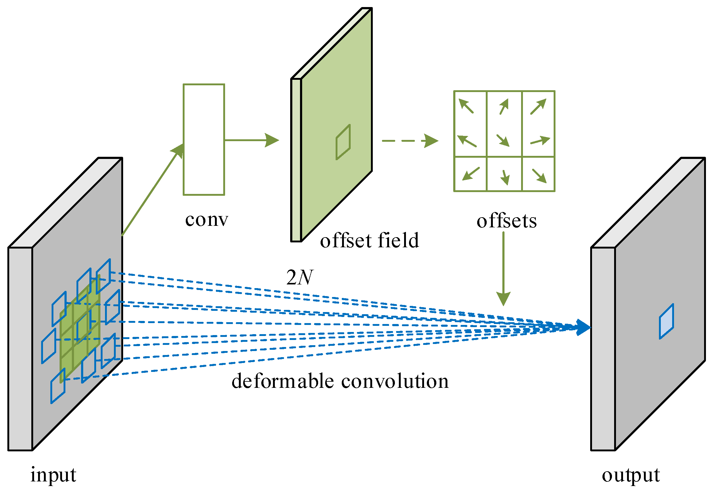
The schematic diagram of deformable convolutional sampling is shown in Figure 3. For the input-feature map, it is assumed that the traditional convolutional network uses a convolutional-kernel size of 3 × 3 to obtain the convolutional-feature map, and the deformable convolution is obtained by an additional kernel of 3 × 3 to learn the offset domain. The offset domain has the same size as the input-feature map, and the number of channels is $2N$, which corresponds to N two-dimensional offset. Then, the output is the result of the joint action of the input-feature map and the offset domain.

3.2. Improved PANet Module

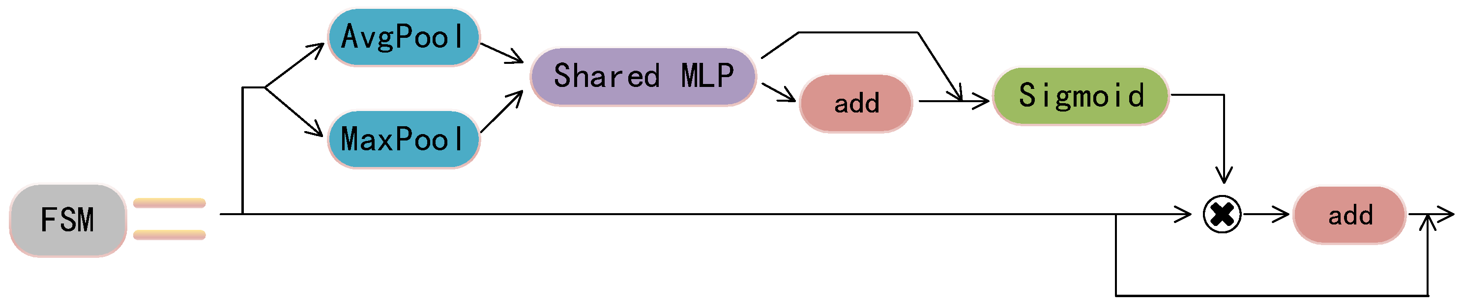
Before performing channel reduction on features, a feature-selection module is proposed to adaptively adjust feature maps that contain excessive spatial details, thereby achieving precise localization and suppressing redundant feature maps. The schematic diagram of the feature-selection module (FSM) is shown in Figure 4. The module first adopts a dual-branch structure, using global-maximum pooling and global-average pooling to extract the information of its feature maps. Then, the output-feature maps are inputted into the MLP structure separately. Then, the two feature maps outputted from the MLP are added and subjected to the sigmoid operation. Finally, the output obtained by multiplying the output-feature maps by the input-feature maps is placed in the input-feature maps and then subjected to the add operation.

The feature-selection module introduces additional skip connections between input- and scaled-feature maps. Using skip connections for scaled features can avoid any specific channel response being excessively amplified or suppressed and can adaptively recalibrate the channel response through channel attention.

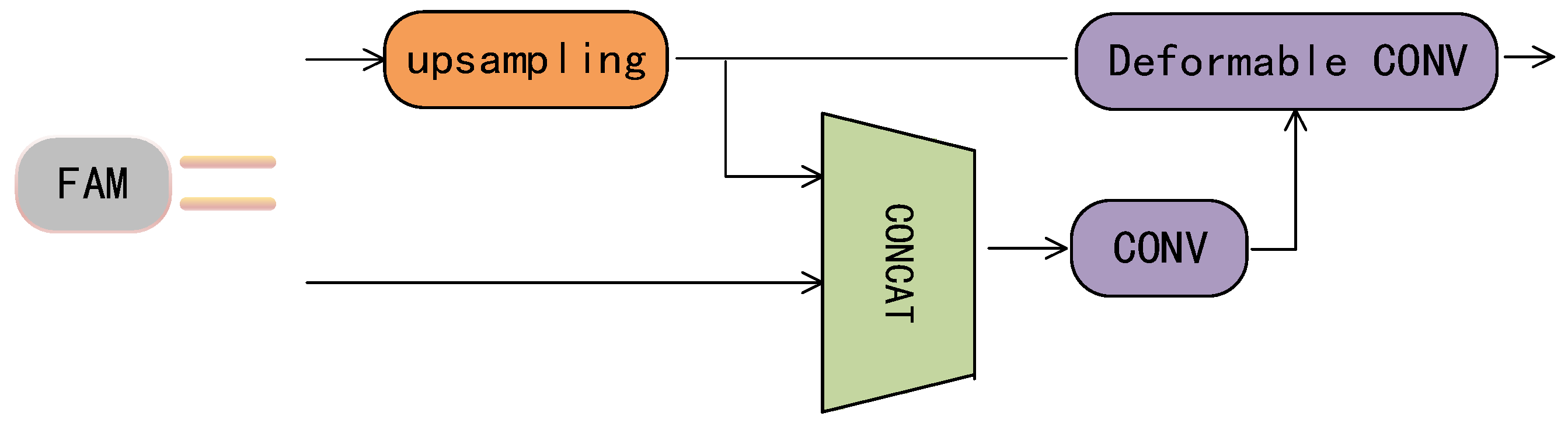
The recursive use of down-sampling and up-sampling operations in deep neural networks may result in spatial misalignment between feature maps, and feature fusion directly through element-level addition or channel-level stitching can affect the detection of object-bounding boxes [28]. A feature-alignment module is proposed to address the above issues. This module can calibrate the underlying features by combining high-level features before feature fusion. The feature-alignment module is shown in Figure 5.

The feature-alignment module up-samples low-level information to ensure consistent feature-map size and then concatenates the feature map with high-level feature maps. The offset is learned through convolution and input into deformable convolution to perform feature alignment on the up-sampled feature map. Spatial-position information is represented through two-dimensional feature maps, where each offset includes the offset distance and corresponding point of each point, as shown in Formulas (6) and (7):

$${\widehat{P}}_i^u=f_a(P_i^u,{\Delta }_i)$$

(6)

$${\Delta }_i=f_o([{\widehat{C}}_{i-1},P_i^u])$$

(7)

${\widehat{C}}_{i-1}$ Represents the (i − 1)th layer feature map, $P_i^u$ represents the result of up-sampling the ith layer feature, and $[{\widehat{C}}_{i-1},P_i^u]$ is a concatenation of ${\widehat{C}}_{i-1}$ and $P_i^u$, which provides the spatial difference between up-sampling and corresponding bottom-up features. $f_a(·)$ and $f_{\mathrm{o}}(·)$ represent the learning offset ${\Delta }_i$ derived from spatial differences and aligned features with the learning offset, respectively.

Using deformable convolution for feature alignment, first, an input-feature map and a convolutional layer are defined, and then, the output features at any position ${\widehat{x}}_P$ are obtained after the convolutional kernel.

$${\widehat{x}}_P={\displaystyle \sum _{n=1}^N{W}_n·x_P+P_n}$$

(8)

N is the size of the convolutional layer, $W_n$ is the weight of the nth convolution, and $P_n$ is the pre-specified offset.

In order to adaptively adjust for different sample positions, in addition to pre-specified offsets, other offsets $\left\{∆p_1,∆p_2,\cdots ,∆p_n\right\}$ need to be learned.

$${\widehat{x}}_P={\displaystyle \sum _{n=1}^N{W}_n·x_P+P_n+}\Delta P_n$$

(9)

Each $\Delta P_n$ is a tuple of $(h,w)$, where $h\in (-H_i,H_i)$, $w\in (-W_i,W_i)$.

The improved YOLOv4 network is shown in Figure 1 and combines the feature-alignment module and feature-selection module to improve the PANet module of YOLOv4. Before the fusion of low-level and high-level features, the up-sampled features of the low-level features and the high-level features are removed from redundant information through the feature-selection module and then input into the feature-alignment module for feature alignment.

3.3. Focal-EIoU Loss Function

The target detection uses bounding-box regression to locate the target in the image, and the early target detection uses IOU as the loss function of the location. However, when the prediction boxing does not overlap the real boxing, the gradient of the IOU loss function disappears, resulting in a slower convergence speed and an inaccurate detector. This inspired several improved loss-function designs based on IOU, including GIOU, DIOU, and CIOU. Whereas GIOU introduces a penalty term in the IOU loss function to alleviate the problem of gradient disappearance, YOLOv4 uses the CIOU loss function. The loss function considers the center-point distance and width–height ratio between the prediction box and the real box in the penalty term, but the relative ratio of width and height is not a very direct indicator, so it is proposed to use the side length as a more direct penalty term. In addition, in order to solve the problem of severe oscillation of loss value caused by low-quality samples, the combination of EIOU loss and focal loss forms the Focal-EIOU loss function.

3.4. Soft-NMS

After the YOLOv4 network detects images, a target may generate a large number of bounding boxes, and the final output is only the optimal bounding box corresponding to the target, which requires a non-maximum-suppression algorithm. This algorithm sorts the confidence levels of all bounding boxes and deletes excess bounding boxes in descending order of confidence levels. The approach of the non-maximum-suppression algorithm in YOLOv4 is to select the bounding box with the highest confidence, calculate the DOIU between the remaining bounding boxes, delete them if they are greater than the set threshold and retain them if they are less than the set threshold, and then select the bounding box with the second highest confidence to perform this operation, and so on until all filtering is completed. The non-maximum-suppression algorithm mainly uses this iterative form to continuously perform DIOU operations with other boxes with the highest confidence and filter out boxes with a larger DIOU.

The specific operation of Soft-NMS has three inputs: detection-box set B, confidence set S, threshold N, and a set D used to store the final detection box. When set B is not empty, the maximum confidence in set S is found. Assuming the subscript of this maximum confidence is m, there is also a corresponding detection box $b_m$ in set B, which is the corresponding detection box for this confidence. Then, detection box $b_m$ in stored in M, and it is merged and delete from the B set. Each detection box $b_m$ is looped through in set B and the DIOU is calculated, and the combined effect of the DIOU value and confidence is used as the final score of the detection box. Formula (10) provides the definition of Soft-NMS as follows in order to change the practice of directly deleting detection boxes with high overlap in NMS and follow the principle that the larger the DIOU, the lower the score:

$$s_i=\left\{\begin{array}{cc}{s}_i,\hfill & \mathit{DIOU}\left(\mathrm{M},b_i\right)<N_t\hfill \\ s_i\left(1-\mathit{DIOU}\left(\mathrm{M},b_i\right)\right),\hfill & \mathit{DIOU}\left(\mathrm{M},b_i\right)\ge N_t\hfill \end{array}\right.$$

(10)

$s_i$ is the confidence level of the object, $\mathrm{DIOU}\left(\mathrm{M},b_i\right)$ represents the size of the DIOU between detection boxes, and $N_t$ is the set threshold.

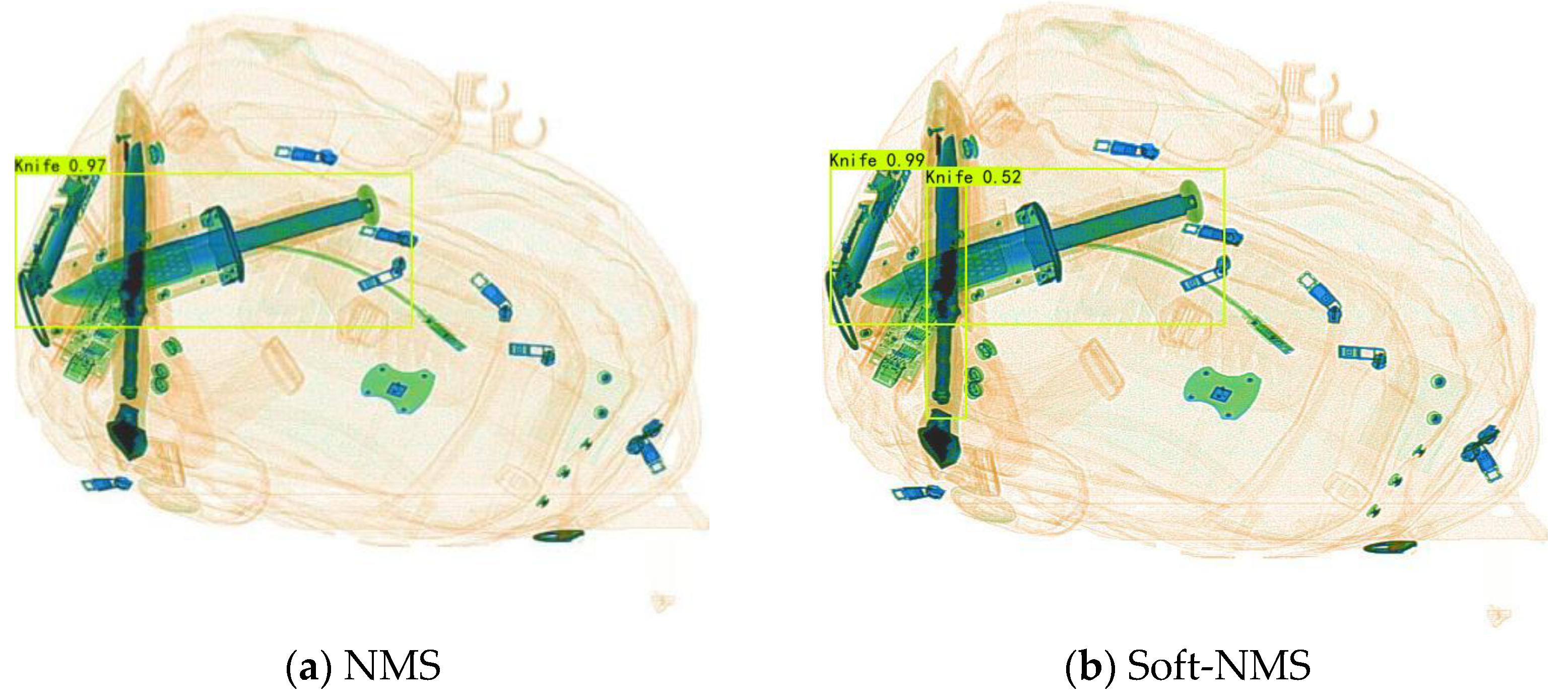
The processing results using two different NMS algorithms are shown in Figure 6. Figure 6a shows the results of the traditional NMS method, which may miss detection when two objects overlap. This is because when two objects overlap, the DIOU threshold is directly used to determine whether to delete the bounding box, which may delete the exact bounding box of the other object. The Soft-NMS algorithm no longer only uses the DIOU to determine whether to delete the bounding box but also considers both the DIOU and the confidence size when deleting the bounding box and gives the correct detection results, as shown in Figure 6b.

3.5. Improved Channel Pruning

There is a large number of redundant parameters in the operation process of convolutional neural networks, which have little effect on improving the detection accuracy of the model and may even lead to a decrease in accuracy. Effectively removing these redundant parameters can improve the detection speed of the network. Channel pruning can delete entire redundant channels while preserving the original convolutional structure, improving network-detection performance without losing accuracy. This design aims to create a channel-pruning method for the YOLOv4-PANv2 network, which considers channel pruning as a search problem, and the legitimate pruning network in the search space is called a subnet. The adaptive BN method is used to evaluate the subnet, which can accurately and quickly find the optimal subnet. The overall pruning process is shown in Figure 7. Firstly, n subnets are generated through the pruning strategy, and each subnet is evaluated by adaptive BN to select the one with the highest score. After several epochs, the pruned model is determined.

The detection accuracy of the subnet generated by the pruning strategy can only be tested after the training process converges. However, each subnet is evaluated by this method, which requires not only fine hyperparameter adjustment but also an extra time-consuming training process. This design uses an adaptive BN-evaluation method that can quickly and accurately select subnets with good final-testing performance. The original BN formula is written as follows:

$$y=\gamma \frac{x-u}{\sqrt{{\sigma }^2+\epsilon }}+\beta$$

(11)

where $\beta$ and $\gamma$ represent the scaling factors and offsets learned through training, respectively, and $\mu$ and ${\sigma }^2$ represent the mean and variance of the current batch for small batch size of N, respectively.

$$u_B=E\left[x_B\right]=\frac{1}{N}{\displaystyle \sum _{i=1}^N{x}_i}$$

(12)

$${\sigma }_B^2=V_{ar}\left[x_B\right]=\frac{1}{N-1}{\displaystyle \sum _{i=1}^N{(x_i-u_B)}^2}$$

(13)

If the same method is used to normalize a batch of samples that need to be predicted during testing, uncertainty occurs in the prediction results. Therefore, during the testing phase, the global-BN statistics are used to calculate ${\mathsf{\mu }}_{\mathrm{T}} \mathrm{a}\mathrm{n}\mathrm{d} {\mathsf{\sigma }}_{\mathrm{T}}^2$ as follows:

$$u_t=m{u}_{t-1}+(1-m)u_B$$

(14)

$${\sigma }_t^2=m{\sigma }_{t-1}^2+(1-m){\sigma }_B^2$$

(15)

where m is the momentum coefficient, and the subscript t represents the number of training iterations. The statistical information of BN is not learned through training but rather is obtained through data statistics. During testing, global-BN statistical information is required to stabilize performance. However, there may be a mismatch between the global-BN statistical information of the pruned subnet and the global-BN statistical information before pruning, leading to unstable detection performance in direct testing. The general method is to train the subnet for several epochs before accurately testing its subnet performance. Adaptive BN inputs data into the network for several epochs of inference, which resamples the subnets and solves the problem of statistical-data mismatch. The use of the adaptive-BN method can quickly select subnets with excellent performance.

4. Results

All experiments in this paper were implemented under the Linux operating system using the Python language and Pytorch framework and a GPU-accelerated NVIDIA A100-PCIe graphics card, and the CPU was Intel(R) Xeon(R) Gold 6330 CPU @ 2.00 GHz.

This paper selected the public dataset Security Inspection X-ray Benchmark (SIXray) for the experiments [24], which was released by the University of Chinese Academy of Sciences. The SIXray dataset contains more than one million security-screening images from subway stations, which provided enough training and testing data. Moreover, the images in the dataset have high clarity and resolution, covering many of the most common items in security tasks. Each image provides detailed labeling information, including the type, location, and size of the items. In this experiment, 8929 positive sample images were used, including five categories of guns, knives, wrenches, pliers, and scissors. The quantity distribution of each category is shown in

Table 1. The distribution of the number of categories in the dataset.

Category	Guns	Knives	Wrenches	Pliers	Scissors
Number	3131	1943	2199	3961	983

.

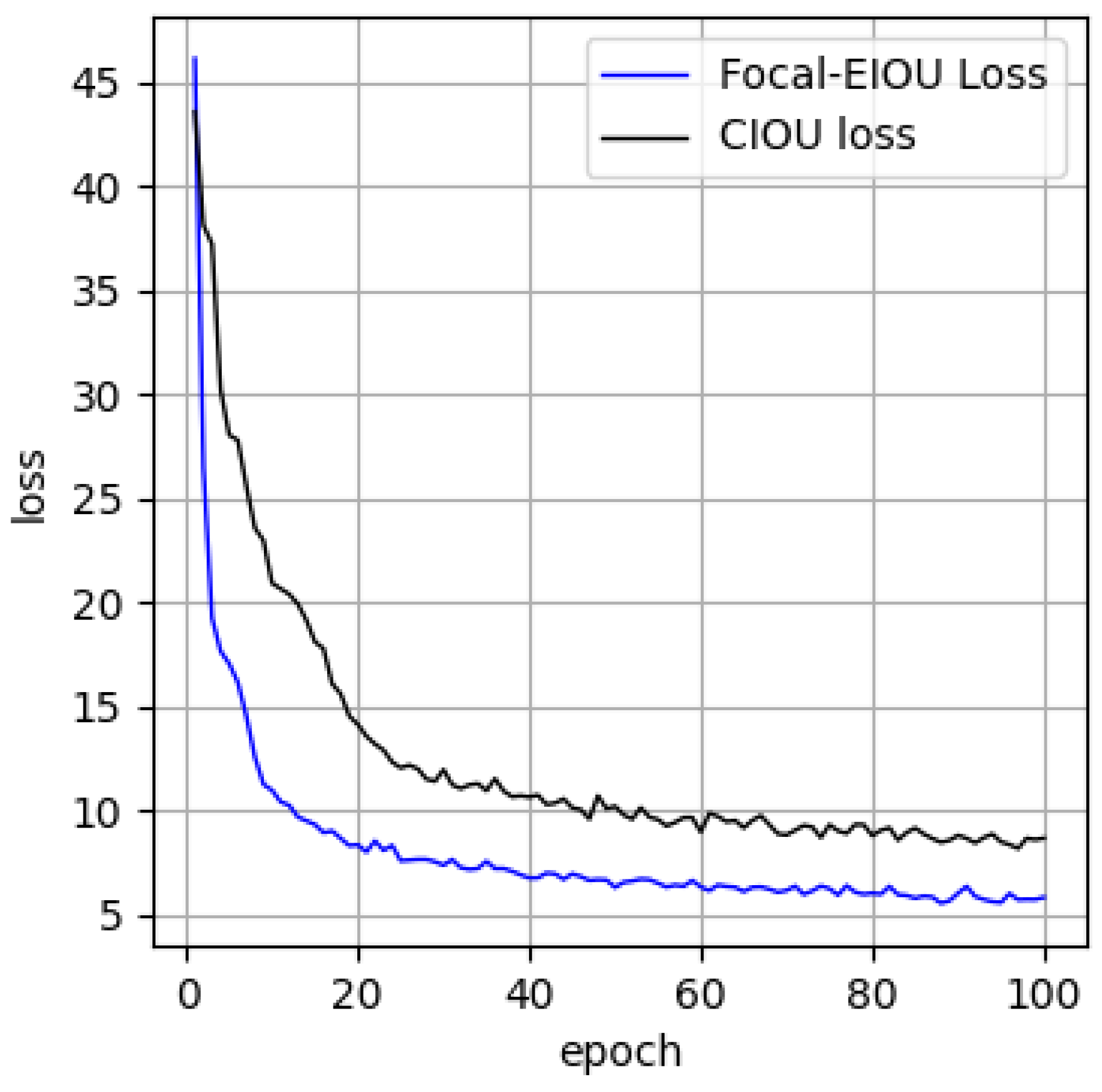
The dataset was divided into two parts, with 80% of the samples as the training set and 20% of the samples as the test set. The maximum learning rate was 1 × 10⁻³, and the minimum learning rate was 1 × 10⁻⁶. Using the label-smoothing strategy and cosine-annealing optimization algorithm, we learned to first simulate the rapid decline of the function and then linearly increase and repeat the process continuously. The epoch was set to 100. First, the influence of the Focal-EIOU loss function on the network was verified. The original CIOU loss function and the Focal-EIOU loss function were used to train the YOLOv4 network. The visualization results of the loss function are shown in Figure 8. The network using the CIOU loss function began to converge to a stable level at the 30th epoch, whereas the network using the Focal-EIOU loss function began to converge at the 19th epoch, indicating that it had a faster convergence rate.

In order to verify the effectiveness of the proposed method in this paper in improving the accuracy of the YOLOv4 network, we compared it with other object-detection models, including YOLOv3, M2Det [29], SSD [30], and YOLOv4, as shown in

Table 2. Detection results with different models.

Method	Guns (%)	Knives (%)	Wrenches (%)	Pliers (%)	Scissors (%)	mAP (%)
YOLOv3	93.18	78.00	68.55	79.69	76.97	79.28
M2Det	95.49	75.70	70.17	83.00	82.96	81.47
SSD	94.91	77.87	74.82	84.51	82.69	82.96
YOLOv4	94.40	81.69	77.38	84.50	77.55	83.11
YOLOv4-PANv2	95.73	83.00	82.95	85.13	80.74	85.51

.

The mAP of the improved model was the highest, reaching 85.51%, which was 6.23%, 4.04%, 2.55%, and 2.4% higher than that of the YOLOv3, M2Det, SSD, and YOLOv4 models, respectively. Compared with YOLOv4, the AP value of guns increased by 1.33%, that of knives increased by 1.31%, that of wrenches increased by 5.57%, that of pliers increased by 0.63%, and that of scissors increased by 3.19%.

In order to further analyze the performance of the different categories, the AP, precision, recall and F1 measure of each category of the YOLOv4-PANv2 network were analyzed, as shown in

Table 3. Improved model-performance analysis for each category.

Category	AP (%)	Precision (%)	Recall (%)	F1 Measure
Guns	95.73	98.59	84.92	0.91
Knives	83.00	91.43	67.20	0.77
Wrenches	82.95	83.66	71.95	0.77
Pliers	85.13	92.95	74.23	0.82
Scissors	80.74	86.88	75.13	0.81

. It can be seen from the table that the AP, precision, recall, and F1 measure of guns were the highest, because the number of gun samples in the dataset was the largest. The recall of knives was relatively low. Because knives are usually thin in shape and can easily overlap with other dangerous goods, there is more missed detection. The precision of the five types of dangerous goods was maintained at a good level, indicating that the model has strong generalization ability and a low false-detection rate.

The average value of various objects was taken as the overall performance-evaluation index and compared with the original YOLOv4, as shown in

Table 4. Comparison of YOLOv4 performance before and after improvement.

Method	mAP (%)	Precision (%)	Recall (%)	F1 Measure
YOLOv4	83.11	90.35	73.00	0.80
YOLOv4-PANv2	85.51	90.70	74.69	0.82

.

As can be seen from the table, compared with the original YOLOv4 model, the mAP, accuracy, and recall rate of the YOLOv4-PANv2 model increased by 2.4%, 0.35%, and 1.69%, respectively, which means that all indicators of our detection algorithm were improved and the improved model had better detection performance.

The detection performance of the model in the test set is shown in Figure 9, where (a) is a single-target image, (b) is a multi-target image, (c) is an occluded-target image, (d) is an overlapping image, (e) is a placement-difference image, and (f) is a small-target image. It can be seen that the improved model could accurately detect each target with our proposed method.

5. Discussion

5.1. Ablation Experiment

In order to verify the model-detection effect after adding different improvement points, ablation experiments and analysis were conducted on the improved PANet module, Focal-EIOU loss function, and Soft-NMS. The comparison results of the ablation experiments are shown in

Table 5. Comparison results of ablation experiment.

Method	Improved PAN	Focal-EIOU Loss	Soft-NMS	mAP (%)
YOLOv4	×	×	×	83.11
YOLOv4-Improved PAN	√	×	×	85.06
YOLOv4-Focal-EIOU Loss	×	√	×	83.96
YOLOv4-Soft-NMS	×	×	√	84.01
YOLOv4-PANv2	√	√	√	85.51

. It can be seen from the table that mAP was significantly improved after the PANet module was improved, indicating that the feature-selection module and feature-alignment module were used in the process of low-level and high-level feature fusion, which significantly improved the detection performance. After using the Focal-EIOU loss function, the model mAP was slightly improved. It can be seen that the Focal-EIOU loss function not only accelerated the convergence of the model but also improved the detection performance of the model. Finally, Soft-NMS also increased the mAP of the model by 0.9%, which more accurately deleted redundant boundary boxes in the processing of images with a high overlap rate.

5.2. Analysis of Channel-Pruning Performance

Although the YOLOv4-PANv2 network improved detection accuracy compared to the YOLOv4 network, the detection speed is not ideal and it would be difficult to meet the detection speed required for X-ray security when there are many bags. To address the above issues, a channel-pruning algorithm was designed to reduce the redundant convolutional channels of the model while not reducing accuracy in order to reduce the computational complexity and improve the detection speed of the model. The distribution of scaling factors before and after sparse training is shown in Figure 10.

Figure 10a shows the distribution of scaling factors in the BN layer during normal training, and Figure 10b shows the distribution of scaling factors in the BN layer during sparse training. The x-axis coordinate represents the size of the scaling factor, the y-axis coordinate represents the epoch of the training, and the z-axis coordinate represents the number of scaling factors. The use of L1 regularization terms effectively suppressed the scaling factor corresponding to channels that made little contribution to the model, making it approach 0. Channels with relatively large contributions also had their scaling factor suppressed, but the final value was also relatively large.

The statistical distribution of the scaling factor is shown in Figure 11. The horizontal axis represents the current epoch, whereas the vertical axis represents the numerical value of the scaling factor. A higher value indicates a higher quantity. In the end, all scaling factors were basically compressed to 0, and sparse training had a significant effect.

To verify the effectiveness of channel pruning, the detection performance of the YOLOv4-PANv2 network before and after pruning was compared. The detection results are shown in

Table 6. Detection results after model pruning.

Method	FLOPs (G)	FPS (f/s)	mAP (%)
YOLOv4-PANv2	60.52	26.71	85.51
Prune-YOLOv4	40.14	50.41	84.78

. From the table, it can be seen that after channel pruning, the model’s FLOPs decreased by 20.38 G, FPS increased by 23.70 f/s, and mAP only decreased by 0.73%, which was acceptable. After pruning, the computational complexity of the model was significantly reduced, and FPS was significantly improved. This is because the channel-pruning algorithm removed many redundant channels, reducing the calculation parameters and the number of calculations, which can effectively improve the detection speed of the model for X-ray security-inspection images.

6. Conclusions

This paper proposes a combination of deformable convolution and the PANet module of the YOLOv4 network, and designs and implements a dangerous-goods-detection algorithm for X-ray security-inspection images. The deformable convolution with a more flexible receptive field is used to solve feature misalignment in the fusion of high- and low-level features of YOLOv4. The pruning strategy uses adaptive BN to evaluate subnets, which can quickly select subnets with good detection results. While ensuring the accuracy of the detection model, it greatly reduces the FLOPs of the model and improves the FPS of the detection model. Experimental results show that our improved YOLOv4 method can effectively improve the accuracy of the detection network and meet the requirements of X-ray security detection in terms of accuracy and speed. Future work will use lightweight methods to reduce the number of parameters and computation while ensuring detection accuracy, making it easier for embedded implementation.