Modeling and Compensation of Inertial Sensor Errors in Measurement Systems

Abstract

In the field of surveying and mapping, inertial sensor deterministic errors are poorly understood, and error calibration and compensation are not carried out. Thus, in this study, the effects of three types of deterministic errors (i.e., bias, scale factor error, and installation error) in a conventional inertial measurement unit (IMU) error model on a navigation system are theoretically deduced and verified by simulation. Subsequently, navigation experiments are carried out to investigate the effects of the three deterministic errors on the navigation system. The experimental results show that the gyro bias has the strongest influence on the navigation and positioning accuracy of the system. Consequently, we designed a two-position continuous calibration scheme to calibrate the IMU. The calibration scheme can simultaneously calibrate the bias error of the gyroscope and the accelerometer. When calibrating the bias error of the 0.005°/h order of magnitude, the maximum relative error is 13.16%, and the rest of the calibration relative errors are less than 10%, which verifies the effectiveness of the calibration path designed in this paper. The system is compensated by using the IMU bias calibration results, and the navigation experiment results show that the position accuracy and heading accuracy are improved by 72.68% and 79.65%, respectively, through the calibration and compensation of IMU bias error. Therefore, the position and heading accuracy of the system will be greatly improved by calibrating and compensating the bias error through the two-position calibration path before the IMU is used.

1. Introduction

Inertial navigation systems are widely used in various positioning and navigation fields to obtain completely independent information on the high-frequency attitude, velocity, and position of a system in real time [1,2]. The strapdown inertial navigation system (SINS) has replaced the platform inertial navigation system in most navigation fields because of its substantially lower volume, weight, and cost and substantially higher reliability. A SINS is directly fixed on a carrier through an inertial measurement unit (IMU). The error in the measurement output of the inertial sensor is compensated for, and the strapdown matrix is then used to change the attitude. Finally, a computer can be used to complete the navigation solution and update and output the navigation solution results in real time. As the IMU is directly fixed on the carrier, the SINS is mainly used to perform error calibration and compensation for the inertial device [3,4,5].

IMUs play an important role in surveying and mapping. IMUs are widely used in mobile measurement [6,7], indoor positioning [8], pipeline measurement [9], mine tunneling [10], railway track geometry measurement [11], integrated navigation [12,13], and other fields. Reference [1] counted different levels of IMU accuracy indicators and application scenarios. In [14], error analysis and modeling of consumer-grade inertial sensors was carried out and the bias-corrected output of tactical-grade inertial navigation equipment was used as a reference true value to perform online calibration of consumer-grade inertial navigation equipment. In [15], a study was performed of the online calibration method of the microelectromechanical system (MEMS) IMU installed on a robot for the surveying and mapping of buildings. The calibration method was found to improve the output accuracy of the attitude information of the MEMS IMU. The yaw prediction accuracy of the robot was increased by 1–2°, thereby providing more accurate lidar point cloud data for information modeling of buildings. In [16], an error correction method was proposed based on a SINS zero-velocity update model with a motion constraint to solve the problem of SINS accumulation error for a shearer. In addition, the IMU can assist RTK measurements by increasing the speed of aligning the bubble to the level of the centering pod in traditional measurement [17]. In [18], a method was proposed to rectify the reduction in the measurement accuracy of the tilt of the centering rod caused by the bias and scale factor error of the accelerometer. A model for the measurement error of the centering rod was established that related the pitch measurement error and the two aforementioned fixed errors of the accelerometer. The model was used to improve the RTK measurement performance. In [19], a three-position on-site calibration method was proposed for a personal navigation system. The method was used to effectively calibrate the biases and scale factor errors of the gyro and accelerometer but did not have ideal accuracy. IMUs are used in novel applications. For example, IMUs are used to determine the attitude of small unmanned aerial vehicles (UAVs) [20] and facilitate human-motion tracking [21]. In [22], yaw-angle estimation was improved for low-cost inertial navigation system/global positioning system (INS/GPS) integration. Seamless integrated navigation of a low-cost multi sensor system was achieved in [23]. In [24], a novel dead reckoning algorithm was proposed for the mapping and positioning of an urban underground pipeline. However, the IMU error was not analyzed. In [25], the filtering algorithm was improved to address the situation of reduced accuracy caused by the replacement of tactical-level IMUs by MEMS in pipeline measurements of small apertures, but this improvement is less helpful for improving the accuracy, and cannot solve the fundamental problem of large, fixed errors of the sensor itself. In [26], an online calibration method for the visual–inertial system was proposed, which has low operability in the field of surveying and mapping. The most effective way to improve the accuracy of the IMU is to calibrate the IMU, but IMU calibration is relatively unfamiliar in the field of surveying and mapping, and there is little demand for high-cost, high-precision calibration solutions [27,28]. Therefore, it is necessary to conduct research on IMU calibration in the field of surveying and mapping and design a calibration scheme that meets the needs of the field of surveying and mapping. Against this research background, an in-depth analysis of the IMU error is conducted in this study to develop an improved calibration scheme for the IMU error.

The error in an inertial navigation system accumulates over time and considerably affects the accuracy of the information output by the system. Calibrating and compensating for the IMU error are highly effective and necessary for improving the system accuracy. IMU errors can be classified into deterministic and random errors [29]. In this paper, firstly, this paper conducts simulation experiments and analysis around the effect of three types of deterministic errors of IMU on the system attitude, velocity, and position navigation accuracy; the discussion and research in this part is for the convenience of researchers who have specific IMU output requirements, such as researchers who only need IMU to output high-precision attitude information. For the field of surveying and mapping, the use scenarios of IMU mainly appear in the low dynamic field, and more attention is paid to plane information, so IMU high-precision position and heading information is especially important. In the following research, we will pay more attention to which error has the greatest impact on the position and heading accuracy of the system among all the errors of the IMU, and then design a calibration for this error to provide a cost-effective calibration solution. The error with the largest effect on the system accuracy is then effectively compensated by calibration of the SINS before use, thereby improving the navigation accuracy.

This paper is organized as follows. In Section 1, IMU error modeling is presented, including a sensor error model and systematic error equations. In Section 2, the effect of the fixed error of the sensor on the system is determined and analyzed. In Section 3, a navigation simulation experiment and IMU error calibration and compensation are described. The study is summarized in Section 4.

2. Materials and Methods

2.1. Sensor Error Model

Inertial sensors generally consist of three accelerometers and three gyros, as shown in Figure 1. Ideally, the components of the accelerometer and gyro assemblies are mounted orthogonally to provide the SINS with information on the acceleration and angular rate of the carrier in three orthogonal directions. The acceleration is integrated once to obtain the carrier velocity, which is in turn integrated to obtain the carrier position. The angular rate provides information on changes in the attitude of the carrier.

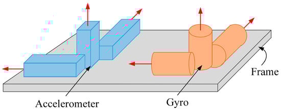
Figure 1. Schematic of the inertial sensor.

The main deterministic errors of inertial sensors are bias, scale factor error, and installation error. Bias is the output level for a zero input to the accelerometer or gyro. Scale factor error is the difference between the scale factors of accelerometer or gyro in actual operation and their factory calibration factors. Installation error is produced by misalignment of the sensitive axes of the accelerometer and gyro with those of the carrier coordinate system (as shown in Figure 2) caused by deviations from ideal installation [30]. In Figure 2, the carrier coordinate system ($o-x_b{y}_b{z}_b$) is triply orthogonal, whereas neither the acceleration coordinate system (composed of the coordinates of the three accelerometers) ($o-x_a{y}_a{z}_a$) or the gyro coordinate system (composed of the coordinates of the three gyros) ($o-x_g{y}_g{z}_g$) is triply orthogonal. Neither $o-x_a{y}_a{z}_a$ nor $o-x_g{y}_g{z}_g$ coincide with $o-x_b{y}_b{z}_b$.

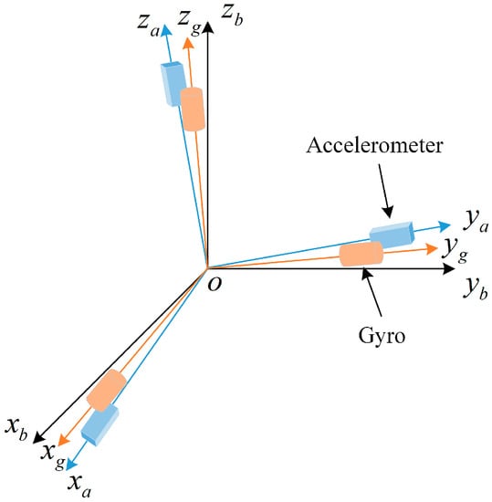
Figure 2. Schematic of IMU installation error.

The output error model of the three-axis accelerometer and three-axis gyro of the SINS is as follows:

$$\left[\begin{array}{c}\delta f_x^b\\ \delta f_y^b\\ \delta f_z^b\end{array}\right]=\left[\begin{array}{ccc}{K}_{ax}& E_{axy}& E_{axz}\\ E_{ayx}& K_{ay}& E_{ayz}\\ E_{azx}& E_{azy}& K_{az}\end{array}\right]\left[\begin{array}{c}{f}_x^b\\ f_y^b\\ f_z^b\end{array}\right]+\left[\begin{array}{c}{B}_{ax}\\ B_{ay}\\ B_{az}\end{array}\right]$$

(1)

$$\left[\begin{array}{c}\delta {\omega }_{ibx}^b\\ \delta {\omega }_{iby}^b\\ \delta {\omega }_{ibz}^b\end{array}\right]=\left[\begin{array}{ccc}{K}_{gx}& E_{gxy}& E_{gxz}\\ E_{gyx}& K_{gy}& E_{gyz}\\ E_{gzx}& E_{gzy}& K_{gz}\end{array}\right]\left[\begin{array}{c}{\omega }_{ibx}^b\\ {\omega }_{iby}^b\\ {\omega }_{ibz}^b\end{array}\right]+\left[\begin{array}{c}{B}_{gx}\\ B_{gy}\\ B_{gz}\end{array}\right]$$

(2)

where $\delta f_I^b(I=x,y,z)$ and $f_I^b(I=x,y,z)$ represent the output errors and ideal output of the accelerometers, respectively; $\delta {\omega }_{ibI}^b(I=x,y,z)$ and ${\omega }_{ibI}^b(I=x,y,z)$ represent the corresponding variables for the gyros; $K_{aI}(I=x,y,z)$ and $K_{gI}(I=x,y,z)$ represent the scale factor errors; $E_{aIJ}(I,J=x,y,z;I\ne J)$ and $E_{gIJ}(I,J=x,y,z;I\ne J)$ represent the installation errors; $B_{aI}(I=x,y,z)$ and $B_{gI}(I=x,y,z)$ represent the bias, where a and g denote the accelerometers and gyros, respectively.

Equations (1) and (2) can be simplified to

$$\left\{\begin{array}{l}\delta {\mathit{f}}^b={\mathit{E}}_a{\mathit{f}}^b+{\mathit{B}}_a\\ \delta {\mathit{\omega }}_{ib}^b={\mathit{E}}_a{\mathit{\omega }}_{ib}^b+{\mathit{B}}_g\end{array}\right.$$

(3)

2.2. Systematic Error Equation

The propagation of the device error of the inertial sensor in the inertial navigation system under the condition of a stationary base is described by systematic error equations, where Equations (4)–(6) model the error in the velocity, attitude, and position, respectively [31,32,33]:

$$\delta {\dot{\mathit{v}}}^n={\mathit{f}}^n\times \mathit{\varphi }+{\mathit{C}}_b^n\delta {\mathit{f}}^b-(2\delta {\mathit{\omega }}_{ie}^n+\delta {\mathit{\omega }}_{en}^n)\times {\mathit{v}}^n-(2{\mathit{\omega }}_{ie}^n+{\mathit{\omega }}_{en}^n)\times \delta {\mathit{v}}^n-\delta {\mathit{g}}^n$$

(4)

$$\dot{\mathit{\varphi }}=\mathit{\varphi }\times {\mathit{\omega }}_{in}^n+\delta {\mathit{\omega }}_{in}^n-{\mathit{C}}_b^n\delta {\mathit{\omega }}_{ib}^b$$

(5)

$$\begin{array}{l}\delta \dot{L}=\frac{\delta v_N}{R_M+h}-\delta h\frac{v_N}{{(R_M+h)}^2}\\ \delta \dot{\lambda }=\frac{\sec L}{R_N+h}\delta v_E+\frac{v_E\sec L\tan L}{R_N+h}\delta L-\frac{v_E\sec L}{{(R_N+h)}^2}\delta h\end{array}$$

(6)

In the equations above, n, I, b, and e represent the navigation frame, inertial frame, body frame, and Earth frame, respectively; $\mathit{\varphi }={[\begin{array}{ccc}{\varphi }_x& {\varphi }_y& {\varphi }_z\end{array}]}^{\mathrm{{\rm T}}}$ is the misalignment angle error; ${\mathit{\omega }}_{in}^n$ denotes the projection of the rotational angular velocity of n-frame relative to i-frame in n-frame; ${\mathit{\omega }}_{ib}^b$ denotes the projection of the rotational angular velocity of b-frame relative to i-frame in b-frame; ${\mathit{C}}_b^n$ represents the strapdown matrix; ${\mathit{v}}^n={[\begin{array}{ccc}{v}_N& v_E& v_U\end{array}]}^{\mathrm{{\rm T}}}$ denotes the projections of the velocity of n-frame relative to e-frame along the north, east, and up directions of n-frame; ${\mathit{f}}^n$ represents the projection of the specific force in n-frame; ${\mathit{\omega }}_{ie}^n$ represents the rotational angular velocity of the Earth in n-frame; ${\mathit{\omega }}_{en}^n$ represents the projection of the rotational angular velocity of n-frame relative to e-frame in n-frame; $\delta {\mathit{g}}^n$ represents the gravity error; $\delta L$ and $\delta \lambda$ represent the latitude and longitude errors, respectively; $R_M$ and $R_N$ represent the radii of curvature of the meridian and prime vertical, respectively.

3. The Influence of Device Error on the System

First, the influence of bias on the system is analyzed. Assuming there is no scale factor error or installation error, the output errors of the accelerometers and gyros are $\delta {\mathit{f}}^b={\mathit{B}}_a$ and $\delta {\mathit{\omega }}_{ib}^b={\mathit{B}}_g$, respectively. Substituting these two results into Equations (4) and (5) yields.

$$\delta {\dot{\mathit{v}}}^n={\mathit{f}}^n\times \mathit{\varphi }+{\mathit{C}}_b^n{\mathit{B}}_a-(2\delta {\mathit{\omega }}_{ie}^n+\delta {\mathit{\omega }}_{en}^n)\times {\mathit{v}}^n-(2{\mathit{\omega }}_{ie}^n+{\mathit{\omega }}_{en}^n)\times \delta {\mathit{v}}^n-\delta {\mathit{g}}^n$$

(7)

$$\dot{\mathit{\varphi }}=\mathit{\varphi }\times {\mathit{\omega }}_{in}^n+\delta {\mathit{\omega }}_{in}^n-{\mathit{C}}_b^n{\mathit{B}}_g$$

(8)

Equation (7) shows that the system velocity error is proportional to the accelerometer bias. Equation (8) indicates that the system attitude error is proportional to the gyro bias. Three sets of accelerometer bias error and three sets of gyroscope bias error are set, respectively, for simulation experiments. Each group of bias errors is separately introduced into the system error model. The settings of three groups of accelerometer bias error and three groups of gyroscope bias error are shown in Table 1. The simulation conditions are set as follows: the initial longitude is 45.78°, the initial latitude is 126.67°, the horizontal attitude angle and attitude error angle are both set to 0°, and the simulation time is 12 h. The simulation experimental results are shown in Figure 3 and Figure 4.

Table 1. Accelerometer and gyroscope bias error simulation settings.

Device	Group	X-Axis/Y-Axis/Z-Axis
Accelerometer	1	100/100/100 μg
	2	200/200/200 μg
	3	300/300/300 μg
Gyro	1	0.01/0.01/0.01°/h
	2	0.02/0.02/0.02°/h
	3	0.03/0.03/0.03°/h

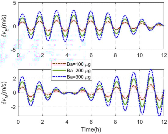
Figure 3. Velocity error introduced by different accelerometer biases.

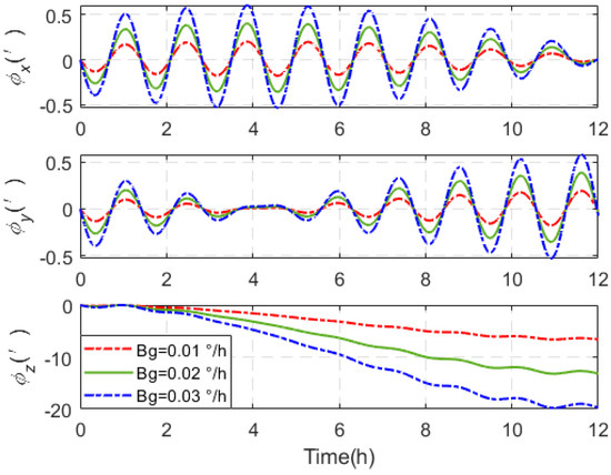
Figure 4. Attitude error introduced by different gyro biases.

Figure 3 and Figure 4 show that as ${\mathit{B}}_a$ and ${\mathit{B}}_g$ increase, the error induced in the speed and attitude increase gradually in a linear relationship with bias errors. In Figure 3 and Figure 4, the speed error and attitude error present a sinusoidal fluctuations pattern over time, which is actually a periodic oscillation. This is because the navigation error caused by the error source includes three types: the Schuler cycle, the Foucault cycle, and the Earth cycle. In terms of periodic oscillators and non-periodic terms, the form of system error oscillation caused by accelerometer zero bias error is the Schuler cycle modulated by Foucault cycle. The form of the system error oscillation caused by the gyroscope zero bias error is that the Schuler periodic oscillation modulated by the Foucault periodic oscillation is superimposed on the Earth periodic oscillation.

Next, the influence of the scale factor error and installation error on the system is analyzed. Assuming there is no bias, the output errors of the accelerometers and gyros are $\delta {\mathit{f}}^b={\mathit{E}}_a{\mathit{f}}^b$ and $\delta {\mathit{\omega }}_{ib}^b={\mathit{E}}_g{\mathit{\omega }}_{ib}^b$, respectively. Substituting these two results into Equations (4) and (5) yields

$$\delta {\dot{\mathit{v}}}^n={\mathit{f}}^n\times \mathit{\varphi }+{\mathit{C}}_b^n{\mathit{E}}_a{\mathit{f}}^b-(2\delta {\mathit{\omega }}_{ie}^n+\delta {\mathit{\omega }}_{en}^n)\times {\mathit{v}}^n-(2{\mathit{\omega }}_{ie}^n+{\mathit{\omega }}_{en}^n)\times \delta {\mathit{v}}^n-\delta {\mathit{g}}^n$$

(9)

$$\dot{\mathit{\varphi }}=\mathit{\varphi }\times {\mathit{\omega }}_{in}^n+\delta {\mathit{\omega }}_{in}^n-{\mathit{C}}_b^n{\mathit{E}}_g{\mathit{\omega }}_{ib}^b$$

(10)

Equations (9) and (10) show that the systematic error resulting from installation error and scale factor error is related to the motion state of the system. The more vigorous the motion is (i.e., the larger ${\mathit{f}}^b$ and ${\mathit{\omega }}_{ib}^b$ are), the larger the systematic error caused by installation error and scale factor error is.

A navigation simulation experiment is carried out, assuming there is no accelerometer bias, for the following scale factor error and installation error:

$${\mathit{E}}_a={\mathit{E}}_g=\left[\begin{array}{ccc}2\times {10}^{-5}& 30″& 30″\\ 30″& 2\times {10}^{-5}& 30″\\ 30″& 30″& 2\times {10}^{-5}\end{array}\right]$$

(11)

Three speeds, 5 m/s, 10 m/s, and 15 m/s, are set to simulate the driving trajectory of a car. The car successively drives 6 km east, 3 km south, 6 km west, and 1.5 km north. The results of the navigation simulation experiment are shown in Figure 5.

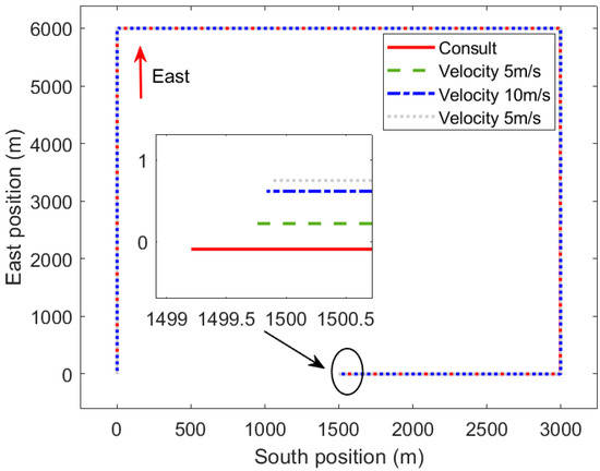
Figure 5. Position error at different vehicle speeds.

Figure 5 shows that for the same driving trajectory, the generated position error varies with the vehicle speed. The position error is smallest at a vehicle speed of 5 m/s and largest at a vehicle speed of 15 m/s. Therefore, the faster the carrier moves, the larger the position error generated by the accelerometer scale factor error and installation error is.

In situ navigation simulation experiments are conducted in swinging and swinging environments with swing amplitudes of 0°, 1°, and 2°. Figure 6 shows the simulation results obtained assuming there is scale factor error and installation error, but no gyro bias, for the parameter setting provided in Equation (11).

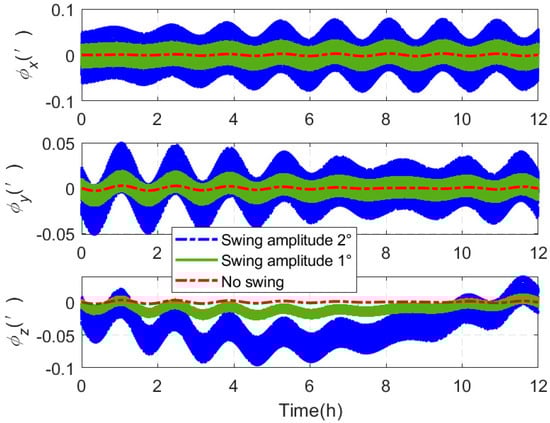
Figure 6. Attitude error generated at different swing amplitudes.

Figure 6 shows that the three angles of the attitude error generated by the gyro scale factor error and installation error increase with the swing amplitude. Therefore, the larger the amplitude of the oscillation of the motion environment of the carrier is and the higher the intensity of the angular motion is, the larger the generated attitude error is.

The effects of the IMU bias, scale factor error, and installation error on the system are analyzed. The scale factor error and installation error produce different effects on the carrier because of differences in the carrier motion. We consider the comprehensive effect of the three types of deterministic IMU errors on the navigation accuracy of the system. What are the individual contributions of the three types of errors to the overall error? Which error has the largest impact on the system accuracy and how can this error be eliminated? These issues are considered in the next section.

4. Navigation Experiment and Error Compensation

4.1. Navigation Simulation Experiment

The three types of deterministic IMU errors produce different effects on the attitude, velocity, and position of the system. Navigation simulation experiments are carried out to investigate the biases, scale factors, and installation errors of the accelerometer and gyro, totaling six types of errors. To determine the error with the largest impact on the system, a simulation is carried out considering each of the six error types and neglecting the effect of the other five error types. Table 2 shows the IMU error parameter settings, which are based on error sizes for common navigation levels. In Table 2, the bias error, scale factor, and installation error are proposed relative to the three axes of the accelerometer frame and the gyroscope frame, and the two frames are a space rectangular coordinate system.

Table 2. Error parameter settings in simulations.

Device	Bias	Scale Factor (ppm)	Installation Error (″)
Accelerometer	100/100/100 μg	20/20/20	30/30/30/30/30/30
Gyro	0.01/0.01/0.01°/h	20/20/20	30/30/30/30/30/30

A long-endurance navigation simulation experiment is carried out for a navigation time of 24 h. The maximum absolute value of each systematic error generated during the navigation period is taken as the systematic error value, and the error results are shown in Table 3. In the field of surveying and mapping, it is mainly vehicle-mounted and ship-mounted IMU. The IMU mainly plays the role of providing navigation position information and heading angle information. It is less dependent on navigation speed information, pitch, and roll information. Therefore, this section mainly studies the position and heading angles. The heading angle is defined as the angle between the $Y_b$-axis of the carrier coordinate system and the north direction of the geographic coordinate system. The heading angle error is the difference between the heading angle result with error and the heading angle result without error. The errors in the position and yaw of the system during navigation caused by the accelerometer and gyro errors are shown in Figure 7 and those caused by the three deterministic errors are shown in Figure 8 and Figure 9. Figure 7 shows that the yaw and position errors caused by the gyro are considerably larger than those caused by the accelerometer. The influence of gyroscope on navigation results is much greater than that of the accelerometer. Therefore, in actual use, more attention should be paid to the accuracy and stability of the gyroscope to ensure the navigation accuracy of the system.

Table 3. Influence of individual error parameters on the system during a long-endurance navigation simulation.

Device	Parameter	Attitude Error (′)			Speed Error (m/s)		Position Error (km)
		Pitch	Roll	Yaw	Eastbound Speed	Northbound Speed	Location
Accelerometer	Bias	0.83	0.83	0.85	1.12	1.12	1.80
	Scale factor	0.03	0.02	0.03	0.03	0.01	1.11
	Installation error	1.21	1.21	1.25	1.63	1.62	2.77
Gyro	Bias	0.20	0.20	6.75	0.85	0.70	26.27
	Scale factor	0.04	0.02	0.03	0.04	0.02	1.67
	Installation error	0.07	0.06	2.08	0.17	0.20	4.34

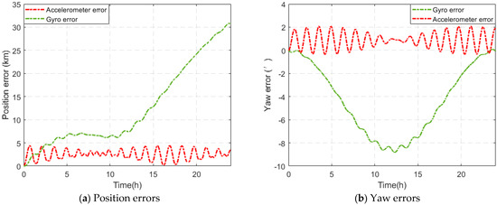
Figure 7. Comparison of errors generated by different devices.

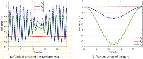
Figure 8. System yaw errors generated by device error parameters.

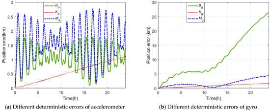
Figure 9. System position errors generated by device error parameters.

Table 3 and Figure 8 and Figure 9 indicate that the different IMU errors impact the navigation accuracy of the system, among which the gyro bias is the largest source of systematic error. Gyro bias generates large errors in the yaw angle and position of the carrier, which is the information most frequently used by the measurement system. Therefore, for practical SINS application, a simple on-site calibration of the gyro bias should be carried out to improve the navigation accuracy of the system.

4.2. Bias Calibration and Compensation

The gyro bias should be quickly calibrated before the field application of IMUs. Positioning precision can be improved by increasing the accuracy of bias results and compensating for the IMU bias. Reference [34] proposed to use two calibration positions to calibrate the bias error, but only three bias errors of the gyroscope can be calibrated. Based on [34], Reference [35] uses three calibration positions with different attitudes to calibrate the bias error of the accelerometer and gyroscope. The calibration scheme is suitable for low-accuracy SINS. In [36], a method for calibrating all the biases of the three-position IMU is proposed. The calibration takes 6 min, but the accelerometer bias error and the gyro bias error are set relatively large. The order of magnitude of the accelerometer bias error is 10⁻¹ °/h, and the order of magnitude of gyro bias error is 10⁻³ g. Two consecutive calibration positions are used in this study. The IMU bias can be completely calibrated by calibrating accelerometer bias during the calibration of the gyro bias.

The calibration scheme is shown in Table 4. The schematic diagram of the calibration is shown in Figure 10. First, the IMU is placed in position one for 10 min. Then, the IMU is rotated counterclockwise around the X-axis by 180° and maintained in position two for 10 min. Passage of the IMU through these two consecutive calibration positions completes calibrations of the six biases.

Table 4. Two-position calibration path scheme.

Position	Three-Axis Orientation	Rotational Axis	Standing Time/(s)
1	North-East-Down	X + 180°	600
2	North-West-Up	-	600

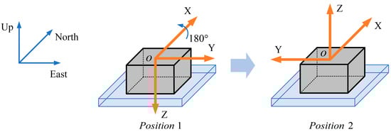
Figure 10. Schematic diagram of the calibration path scheme. The aforementioned calibration path is used to carry out four calibration simulation experiments for a simulation time of 20.5 min. The IMU remains stationary for 10 min at each of the two calibration positions and is rotated 180° around the X-axis for 30 s. The settings of the biases to be calibrated and the simulation results are shown in Table 5, and the default setting of IMU scale factor error and installation error are present and are shown in Table 2. Only the IMU bias calibration result is output during calibration. The maximum relative errors in the gyro and accelerometer calibration results for each experiment are shown in Figure 11.

One of the difficulties in the calibration path is to achieve effective calibration for errors of a much smaller order of magnitude. The calibration path designed in this paper can effectively calibrate the accelerometer bias error of 5 × 10⁻³°/h and the gyro bias error of 5 × 10⁻⁵ g. Table 5 shows that the maximum relative error in the bias calibration for the four calibration experiments is 13.6% and all the results meet the requirements for practical use, which verifies the feasibility of the calibration scheme. The largest relative error is obtained for Experiment No. 1 (as shown in Figure 11), because the biases in this experiment are small in magnitude and, therefore, relatively difficult to calibrate. The calibration scheme adequately meets the requirements of bias calibration of the IMU of the INS.

Table 5. IMU bias error parameter calibration results.

No.	Preset	Estimation
1	50/50/50 (μg)	53.06/46.51/46.34 (μg)
	0.005/0.005/0.005 (°/h)	0.00499/0.00503/0.00432 (°/h)
2	100/100/100 (μg)	103.21/96.48/96.33 (μg)
	0.01/0.01/0.01 (°/h)	0.0099/0.0100/0.0096 (°/h)
3	500/500/500 (μg)	504.24/496.05/496.27 (μg)
	0.05/0.05/0.05 (°/h)	0.0499/0.0499/0.0498 (°/h)
4	1000/1000/1000 (μg)	1005.49/995.41/996.29 (μg)
	0.1/0.1/0.1 (°/h)	0.100/0.099/0.099 (°/h)

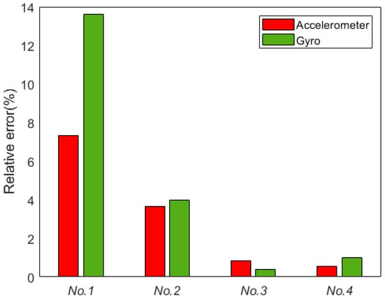
Figure 11. Relative error in calibration results.

Taking the gyro bias shown in Table 2 as an example, simulation experiments are carried out with 90%, 80%, 70%, and 60% compensation of the gyro bias. The experimental results are shown in Figure 12.

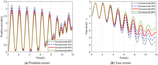
Figure 12. Partial compensation of the gyro bias.

Figure 12 shows that partial compensation of the gyro bias can improve the navigation accuracy of the system even when there are errors in the calibration bias. The accuracy of the position and yaw of the system increases with the calibration accuracy of the bias.

Navigation experiments are carried out using the various IMU error settings shown in Table 1. First, the navigation results for the system position are output without compensating for the IMU errors (including the bias). Second, the bias calibration results of Experiment No. 2, shown in Table 4, are used to compensate for the IMU outputs before outputting the navigation results. Figure 13 shows the combined results for a 12-h navigation without and with bias compensation.

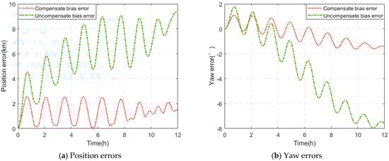
Figure 13. Results of a 12-h navigation experiment.

Figure 13 shows that bias compensation considerably improves the positional navigation accuracy of the system. The maximum position error during the 12-h navigation period is reduced from 9.37 km to 2.56 km, and bias compensation improves the navigation accuracy by 72.68%. The maximum yaw error is reduced from 7.96′ to 1.62′ during the 12-h navigation period, and bias compensation improves the yaw accuracy by 79.65%. Hence, the navigation accuracy of the system can be effectively improved by compensating the IMU outputs using the IMU bias calibration results of the two-position consecutive calibration scheme.

5. Conclusions

A theoretical analysis and experiments on deterministic IMU errors show that the systematic error generated by the IMU bias is proportional to the bias itself, whereas the systematic error generated by scale factor error and installation error is related to the motion state of the carrier (the more intense the motion is, the larger the systematic error is). This helps users who have specific needs for IMUs to pay attention to IMU errors according to their own needs and application scenarios. Next, navigation simulation experiments are carried out to determine the influences of various deterministic errors on the navigation system. The results show that among various deterministic errors, the gyro zero bias error has the greatest impact on the position information and navigation information concerned in the field of surveying and mapping, which is greater than the sum of the impacts of other errors. Aiming at this situation, an on-site calibration method is designed, which only needs two calibration positions for a total of 20.5 min to complete the calibration of the IMU zero bias error. The simulation experiment shows that this calibration path can effectively calibrate the error with a smaller order of magnitude. The relative error of most error calibrations is less than 10%. The system is compensated by using the IMU’s bias error calibration results, the position accuracy is increased by 72.68%, and the heading accuracy is increased by 79.65%. By calibrating and compensating the IMU bias error before use, the navigation accuracy of the system can be improved economically and effectively. This paper provides a reference for the simple and effective calibration of the IMU in the field of surveying and mapping.

References

- Ei-Sheimy, N.; Youssef, A. Inertial sensors technologies for navigation applications: State of the art and future trends. Satell. Navig. 2020, 1, 2. [Google Scholar] [CrossRef]
- Cai, Q.; Yang, G.; Song, N.; Liu, Y. Systematic calibration for ultra-high accuracy inertial measurement units. Sensors 2016, 16, 940. [Google Scholar] [CrossRef] [PubMed]
- Peng, C.; Huang, J.; Lee, H. Design of an embedded icosahedron mechatronics for robust iterative IMU calibration. IEEE-ASME Trans. Mechatron. 2022, 27, 1467–1477. [Google Scholar] [CrossRef]
- Wen, Z.; Yang, G.; Cai, Q.; Sun, Y. Modeling and calibration of the gyro-accelerometer asynchronous time in dual-axis RINS. IEEE Trans. Instrum. Meas. 2021, 70, 3503117. [Google Scholar] [CrossRef]
- Xu, B.; Wang, L.; Duan, T. A novel hybrid calibration method for FOG-based IMU. Measurement 2019, 147, 106900. [Google Scholar] [CrossRef]
- Sairam, N.; Nagarajan, S.; Ornitz, S. Development of mobile mapping system for 3D road asset inventory. Sensors 2016, 16, 367. [Google Scholar] [CrossRef]
- Niu, X.; Wang, Y.; Kuang, J. A pedestrian POS for indoor mobile mapping system based on foot-mounted visual-inertial sensors. Measurement 2022, 199, 111559. [Google Scholar]
- Ei-Sheimy, N.; Li, Y. Indoor navigation: State of the art and future trends. Satell. Navig. 2021, 2, 7. [Google Scholar] [CrossRef]
- Chen, Q.; Zhang, Q.; Niu, X.; Wang, Y. Positioning accuracy of a pipeline surveying system based on MEMS IMU and odometer: Case study. IEEE Access 2019, 7, 104453–104461. [Google Scholar] [CrossRef]
- Wang, S.; Wang, S. Improving the shearer positioning accuracy using the shearer motion constraints in longwall panels. IEEE Access 2020, 8, 52466–52474. [Google Scholar] [CrossRef]
- Chen, Q.; Zhang, Q.; Niu, X.; Liu, J. Semi-analytical assessment of the relative accuracy of the GNSS/INS in railway track irregularity measurements. Satell. Navig. 2021, 2, 25. [Google Scholar] [CrossRef]
- Liu, Y.; Fan, X.; Lv, C.; Wu, J.; Li, L.; Ding, D. An innovative information fusion method with adaptive Kalman filter for integrated INS/GPS navigation of autonomous vehicles. Mech. Syst. Signal Process. 2018, 100, 605–616. [Google Scholar] [CrossRef]
- Chen, C.; Chang, G. Low-cost GNSS/INS integration for enhanced land vehicle performance. Meas. Sci. Technol. 2019, 31, 035009. [Google Scholar] [CrossRef]
- Jin, J.; Zhu, F.; Tao, X.; Liu, W.; Zhang, X. Dynamic systematic error analysis and modeling for consumer inertial sensor. Sci. Surv. Mapp. 2022, 47, 55–61. [Google Scholar]
- Li, S.; Niu, Y.; Feng, C.; Liu, H.; Zhang, D.; Qin, H. An onsite calibration method for MEMS-IMU in building mapping fields. Sensors 2019, 19, 4150. [Google Scholar] [CrossRef]
- Yang, H.; Li, W.; Luo, T.; Luo, C.; Liang, H.; Zhang, H.; Gu, Y. Research on the strategy of motion constraint-aided ZUPT for the SINS positioning system of a shearer. Micromachines 2017, 8, 340. [Google Scholar] [CrossRef]
- Weng, Y.; Wang, S.; Zhang, H.; Gu, H.; Wei, X. A high resolution tilt measurement system based on multi-accelerometers. Measurement 2017, 109, 215–222. [Google Scholar] [CrossRef]
- Dai, M.; Pan, X.; Yang, Y.; Li, Z.; Zhu, Y. A method for improving the performance of centering rod surveying based on two-position correction. Meas. Sci. Technol. 2022, 33, 085001. [Google Scholar] [CrossRef]
- Lu, J.; Lei, C. Applied system-level method in calibration validation for personal navigation system in field. IET Sci. Meas. Technol. 2017, 11, 103–110. [Google Scholar] [CrossRef]
- Strohmeier, M.; Montenegro, S. Coupled GPS/MEMS IMU attitude determination of small UAVs with COTS. Electronics 2017, 6, 15. [Google Scholar] [CrossRef]
- Xu, C.; He, J.; Zhang, X.; Zhou, X.; Duan, S. Towards human motion tracking: Multi-sensory IMU/TOA fusion method and fundamental limits. Electronics 2019, 8, 142. [Google Scholar] [CrossRef]
- Cui, C.; Zhao, J.; Hu, J. Improving robustness of the MAV yaw angle estimation for low-cost INS/GPS integration aided with tri-axial magnetometer calibrated by rotating the ellipsoid model. IET Radar Sonar Navig. 2020, 14, 61–70. [Google Scholar]
- Li, N.; Guan, L.; Gao, Y.; Du, S.; Wu, M.; Guang, X.; Cong, X. Indoor and outdoor low-cost seamless integrated navigation system based on the integration of INS/GNSS/LIDAR system. Remote Sens. 2020, 12, 3271. [Google Scholar] [CrossRef]
- Wei, X.; Fan, S.; Zhang, Y.; Chang, L.; Wang, G.; Shen, F. Positioning algorithm of MEMS pipeline inertial locator based on dead reckoning and information multiplexing. Electronics 2022, 11, 2931. [Google Scholar] [CrossRef]
- Yang, Y.; Li, B.; Wu, X.; Yang, L. Application of adaptive cubature kalman filter to in-pipe survey system for 3D small-diameter pipeline mapping. IEEE Sens. J. 2020, 20, 6331–6337. [Google Scholar] [CrossRef]
- Xiao, Y.; Ruan, X.; Chai, J.; Zhang, X.; Zhu, X. Online IMU Self-Calibration for Visual-Inertial Systems. Sensors 2019, 19, 1624. [Google Scholar] [CrossRef]
- Chang, J.; Fan, S.; Zhang, Y.; Li, J.; Shao, J.; Xu, D. A time asynchronous parameters calibration method of high-precision FOG-IMU based on a single-axis continuous rotation scheme. Meas. Sci. Technol. 2023, 34, 055108. [Google Scholar] [CrossRef]
- Zha, F.; Chang, L.; He, H. Comprehensive Error Compensation for Dual-Axis Rotational Inertial Navigation System. IEEE Sens. J. 2020, 20, 3788–3802. [Google Scholar] [CrossRef]
- Ei-Sheimy, N.; Hou, H.; Niu, X. Analysis and modeling of inertial sensors using Allan variance. IEEE Trans. Instrum. Meas. 2008, 57, 140–149. [Google Scholar] [CrossRef]
- Zhao, G.; Tan, M.; Guo, Q.; Wu, C. An improved system-level calibration method of strapdown inertial navigation system based on matrix factorization. IEEE Sens. J. 2022, 22, 14986–14996. [Google Scholar] [CrossRef]
- Wang, Z.; Xie, Y.; Yu, X.; Fan, H.; Wei, G.; Wang, L.; Fan, Z.; Wang, G.; Luo, H. A system-level calibration method including temperature-related error coefficients for a strapdown inertial navigation system. Meas. Sci. Technol. 2021, 32, 115117. [Google Scholar] [CrossRef]
- Zheng, Z.; Han, S.; Zheng, K. An eight-position self-calibration method for a dual-axis rotational Inertial Navigation System. Sens. Actuators A Phys. 2015, 232, 39–48. [Google Scholar] [CrossRef]
- Wang, B.; Ren, Q.; Deng, Z.; Fu, M. A self-calibration method for nonorthogonal angles between gimbals of rotational inertial navigation system. IEEE Trans. Ind. Electron. 2015, 62, 2353–2362. [Google Scholar] [CrossRef]
- Li, J.; Fang, J.; Du, M. Error analysis and gyro-bias calibration of analytic coarse alignment for airborne POS. IEEE Trans. Instrum. Meas. 2012, 61, 3058–3064. [Google Scholar]
- Lu, J.; Lei, C.; Li, B.; Wen, T. Improved calibration of IMU biases in analytic coarse alignment for AHRS. Meas. Sci. Technol. 2016, 27, 075105. [Google Scholar] [CrossRef]
- Wang, S.; Yang, G.; Wang, L.; Liu, P. A fast calibration method for the all biases of IMU. J. Chin. Inert. Technol. 2020, 28, 316–322. [Google Scholar]
Disclaimer/Publisher’s Note: The statements, opinions and data contained in all publications are solely those of the individual author(s) and contributor(s) and not of MDPI and/or the editor(s). MDPI and/or the editor(s) disclaim responsibility for any injury to people or property resulting from any ideas, methods, instructions or products referred to in the content. |
© 2023 by the authors. Licensee MDPI, Basel, Switzerland. This article is an open access article distributed under the terms and conditions of the Creative Commons Attribution (CC BY) license (https://creativecommons.org/licenses/by/4.0/).