Plane-Wave Generation through General Near-Field In-Band Reflectarray Direct Layout Optimization with Figure of Merit Constraints in mm-Wave Band

Abstract

A general near-field (NF) in-band synthesis strategy is presented for the direct layout optimization (DLO) of reflectarrays with application to the generation of plane waves for the mm-wave band. The technique relies on the definition of relevant figures of merit (FoM) and the use of a gradient-based minimization algorithm. To this end, the volume where the NF is computed is divided into a number of disjoint regions where the FoM are defined. These FoM define the performance of the antenna and their direct optimization enables improvement compared to previous approaches described in the literature, while reducing the memory footprint of the algorithm and accelerating computation. The optimization procedure is divided into several stages to facilitate convergence towards a successful outcome. First, a phase-only synthesis is carried out at a single frequency. Then, a reflectarray layout is obtained using a method of moments based on local periodicity, accounting for mutual coupling between elements. Finally, an in-band DLO is performed at a number of frequencies directly optimizing the FoM. The results show that the obtained reflectarray layout complies with the requirements in the frequency range 27 GHz–29 GHz within the 5G new radio n257 band.

1. Introduction

With the deployment of 5G networks [1], there is an increased need for the electromagnetic characterization of devices for applications that range from the Internet of Things [2,3], smart cities [4], Industry 4.0 [5] and self-driving cars [6], satellite-terrestrial relay networks [7,8] and beam-forming for mm-wave networks [9], among others [10]. Of particular interest is the mm-wave frequency range (FR) 2, from 24.25 GHz to 71 GHz, since it provides a readily available wide spectrum, unlike FR1 in the sub-6 GHz spectrum, which is already very crowded with services that range from wireless local area networks to aerial communications [11]. Of all the FR2 bands, the lower bands around 28 GHz are especially appealing since they have been allocated by the most countries, including, but not limited to, the European Union, the United States, Japan, China and South Korea [11], but also because they present relatively low attenuation losses compared to other mm-wave frequencies [12]. Thus, antenna measurement systems must evolve to fulfil the characterization needs of the devices developed for these new applications.

To this end, a number of alternatives have been proposed for the measurement of radiation patterns at mm-wave bands [12,13,14,15]. However, most of these techniques involve a last stage of data post-processing to obtain the radiation pattern. Another alternative consists in directly acquiring the radiation pattern, for instance, with far-field (FF) ranges. However, since the antenna under test (AUT) needs to be placed in the FF region of the probe, FF ranges usually result in bulky systems. By placing the AUT in the near-field (NF) region of the probe a near-field range is obtained, but, again, data post-processing is required. In this regard, compact antenna test ranges (CATR) [16] solve these issues by simulating open range conditions in the Fresnel region of the probe so the far field may be readily acquired in a close range. Typically, parabolic antennas have been employed, due to their geometrical properties, for the collimation of spherical waves into planar waves in a region known as the quiet zone (QZ) [17]. To avoid diffraction effects due to the low illumination taper in the reflector surface, serrated edges are employed [18]. However, CATR systems based on single or multiple parabolic reflectors have various drawbacks: they are bulky and expensive to manufacture, especially at high frequencies at which the required surface error is very low [16].

A more interesting approach is the use of plane-wave generators (PWG). They consist of array antennas that are optimized to generate a plane wave in their NF region. Although the concept is not new [19,20], it has gained traction in the past few years for over-the-air measurements of 5G devices in the mm-wave ranges [21,22]. The use of conventional arrays generates an issue of requiring complex feeding networks to control the excitation of the array elements [21]. This, in turn, may make the in-band synthesis of these arrays more challenging since the feeding network would, ideally, have to be considered in the simulations to obtain more accurate results [23]. Using spatially fed arrays [24] overcomes this limitation, since the feed may be readily included in the in-band synthesis procedure simply by obtaining the incident field at the array aperture at a number of frequencies, either by means of measurements or use of full-wave simulations. Then, the array element may be easily simulated by assuming local periodicity according to the Floquet theorem [25,26]. Both reflectarrays [27,28,29] and transmitarrays [30,31] have been proposed for use as probes in CATR systems. However, due to the strong illumination taper imposed by the feed, an NF synthesis technique is necessary to shape the NF field in the QZ such that it complies with the requirements of a plane wave.

Recently, several synthesis techniques were proposed for the NF-shaping of spatially fed arrays [28,32,33,34]. The generalized intersection approach (GIA) was employed to carry out a phase-only synthesis (POS) in [28] to design a reflectarray for a CATR system. The technique imposes magnitude and phase constraints by means of lower and upper mask templates at a single NF plane and frequency. The same technique was also employed in NF magnitude-only optimizations for reflectarray [32] and transmitarray [34] antennas. Similarly, in [33] magnitude NF requirements are also specified as mask templates on a whole NF plane. However, the POS is carried out by computing the FF generated by the truncated NF according to those masks as an intermediate step before recovering the field at the array aperture, from which the NF is computed again to assess if it complies with specifications.

The above-mentioned techniques are able to effectively shape the NF, although they present several drawbacks. First, all of them perform a POS and, thus, the procedure only works at a single frequency. Due to the narrow bandwidth nature of spatially fed arrays [35], this may penalize performance at other frequencies. In addition, the GIA employed in [28,32,34] uses a gradient-based technique in the backward projector, which calculates the Jacobian matrix of a cost function. The size of this matrix directly depends on the number of optimizing variables and the number of points at which the NF is calculated, since specifications are implemented with the mask template in all NF points, causing an important memory footprint and slower computations when the NF field is computed in more than one NF plane. On the other hand, the technique employed in [33] avoids the use of a gradient-based algorithm by computing the FF as an intermediate step. However, this limits the technique to the synthesis of NF planes at a single plane parallel to the array. In addition, the technique has only been developed for magnitude-only synthesis, with no NF phase constraints, so it cannot be applied to optimize spatially fed arrays for CATR applications.

In view of these limitations, the present paper proposes a new NF in-band synthesis technique for the optimization of reflectarray antennas with general NF constraints in both magnitude and phase. With the proposed technique, and employing a full-wave simulation tool directly in the optimization loop, an in-band synthesis at a number of frequencies is possible. Moreover, there are no restrictions as to at which points the NF is optimized. In addition, to overcome the memory footprint and slower computations derived from the definition of NF constraints by means of upper and lower mask templates for all NF points, the direct optimization of the relevant NF figures of merit (FoM) in both magnitude and phase is proposed. To this end, the volume where the NF is calculated is divided into a series of disjoint regions where these FoM are calculated. A gradient-based minimization algorithm is adopted to take into account these FoM, considerably reducing the memory footprint and accelerating computations. In addition, a comparison with the usual approach described in the literature of employing mask templates in all the NF points shows that the new methodology is able to produce better results in fewer iterations in the final optimized reflectarray, generating a plane wave with lower magnitude and phase ripple.

2. General Near-Field Synthesis Based on the Optimization of Relevant Figures of Merit

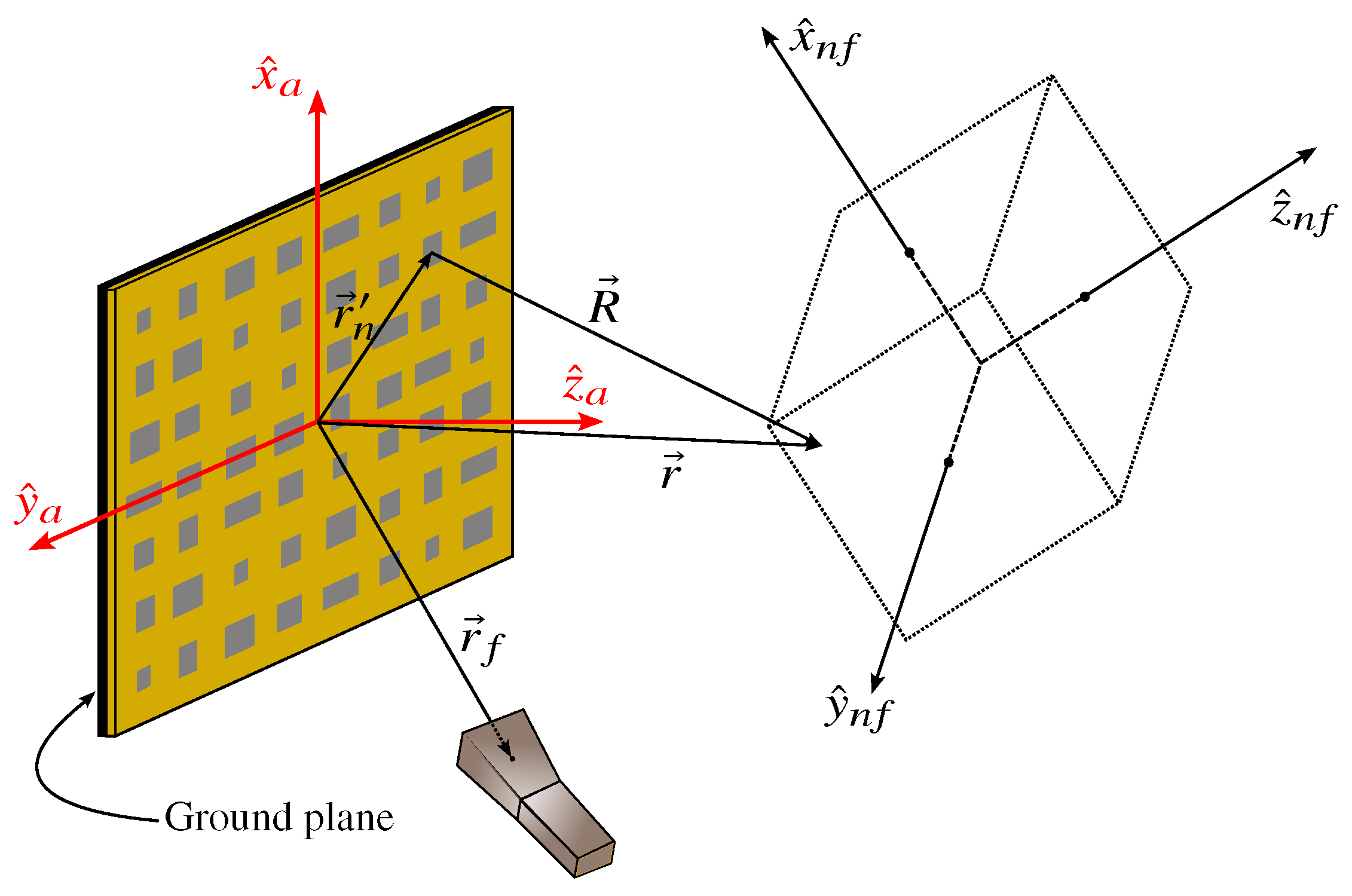
2.1. Calculation of the near Field and Figures of Merit

Let us consider the scenario shown in Figure 1. It consists of a reflectarray comprised of a total of N elements with regular periodicity $p_x\times p_y$, illuminated by a feed whose phase center is placed at ${\overrightarrow{r}}_f$ with regard to the array coordinate system (ACS) defined by $(x_a,y_a,z_a)$. The reflectarray generates a near field in a volume in front of the antenna. Each point in space where the near field is computed is given by $\overrightarrow{r}=(x,y,z)$. In addition, the near field is referenced, in general, to its own coordinate system (NFCS, or near-field coordinate system) given by $(x_{nf},y_{nf},z_{nf})$ which in general is translated and rotated with respect to the ACS.

For a given point in space, the near field radiated by the reflectarray may be obtained as the contribution of the far field radiated by each element:

$${\overrightarrow{E}}_{\mathrm{NF}}\left(\overrightarrow{r}\right)=E_{\mathrm{NF},x}{\widehat{x}}_{nf}+E_{\mathrm{NF},y}{\widehat{y}}_{nf}+E_{\mathrm{NF},z}{\widehat{z}}_{nf}=T\sum _{n=1}^N{\overrightarrow{E}}_{\mathrm{FF},n}(\overrightarrow{r},{\overrightarrow{r}}_n^{\prime }),$$

(1)

where T is the matrix of change of coordinates from the ACS to the NFCS, which is defined by three angles ($\theta ,\phi ,\psi$); ${\overrightarrow{E}}_{\mathrm{FF},n}(\overrightarrow{r},{\overrightarrow{r}}_n^{\prime })$ is the far field generated by the n-th element according to Love’s principle of equivalence [36]; and ${\overrightarrow{r}}_n^{\prime }=(x_n,y_n)$ are the coordinates of the n-th element in the reflectarray coordinate system (see Figure 1). Further details on the near-field model, including the definition of matrix T, may be consulted in [24].

From the near field ${\overrightarrow{E}}_{\mathrm{NF}}\left(\overrightarrow{r}\right)$ obtained in a volume $\mathsf{\Omega }$ in space, the next step is to obtain the relevant FoM. For this purpose, we consider a number of disjoint regions ${\mathsf{\Omega }}_m$, $m=1,2,\dots ,M$ where those FoM may be calculated. These regions fulfil the following properties:

$${\mathsf{\Omega }}_i\cap {\mathsf{\Omega }}_j=\varnothing ;i,j=1,2,\dots ,M;i\ne j,$$

(2a)

$$\mathsf{\Omega }=\bigcup _{m=1}^M{\mathsf{\Omega }}_m,$$

(2b)

where ∅ is the empty set. In short, these two properties mean that the regions ${\mathsf{\Omega }}_m$ fill all space $\mathsf{\Omega }$ without overlapping. Once the regions ${\mathsf{\Omega }}_m$ have been established, we can define the FoM on them. In general, the FoM will be a function f of the near field and, here, we employ the following notation:

$$F_{k,{\mathsf{\Omega }}_m}=f\left\{{\overrightarrow{E}}_{\mathrm{NF}}\left(\overrightarrow{r}\right)\right\},$$

(3)

where $F_{k,{\mathsf{\Omega }}_m}$, $k=1,2,\dots ,K$ is the k-th FoM of a total of K FoM and it is defined in region ${\mathsf{\Omega }}_m$. Since we consider a general NF synthesis with magnitude and/or phase specifications, the FoM can be related to either or both.

The definition of each particular FoM will depend on the goal of the optimization procedure. For instance, one may want to maximize the value of the near field in a particular region, for instance, of the ${\widehat{x}}_{nf}$ component for linear polarization X. Since, for this case, the limiting FoM is the minimum value of the NF, the relevant FoM is:

$$F_{k,{\mathsf{\Omega }}_m}=\underset{{\mathsf{\Omega }}_m}{\min }\left\{|E_{\mathrm{NF},x}|\right\},$$

(4)

where ${\min }_{{\mathsf{\Omega }}_m}$ gives the minimum value in region ${\mathsf{\Omega }}_m$. In this way, one may maximize the minimum value of the field through the proper definition of the FoM. In the case of the present investigation, plane-wave generators usually define the QZ to fulfil specifications with a maximum ripple of phase of 10° and a maximum ripple of magnitude of 1 dB [27,37]. For the magnitude, this FoM is defined, in linear scale, as:

$${\Delta }_{k,{\mathsf{\Omega }}_m}^m=F_{k,{\mathsf{\Omega }}_m}={\displaystyle \frac{{\max }_{{\mathsf{\Omega }}_m}\left\{|E_{\mathrm{NF},x}|\right\}}{{\min }_{{\mathsf{\Omega }}_m}\left\{|E_{\mathrm{NF},x}|\right\}}},$$

(5)

while for the phase is:

$${\Delta }_{k,{\mathsf{\Omega }}_m}^p=F_{k,{\mathsf{\Omega }}_m}=\underset{{\mathsf{\Omega }}_m}{\max }\left\{\angle E_{\mathrm{NF},x}\right\}-\underset{{\mathsf{\Omega }}_m}{\min }\left\{\angle E_{\mathrm{NF},x}\right\}.$$

(6)

The FoM in (5) and (6) are defined for linear X polarization since the x component of the field is used. Analogous FoM may be defined for Y polarization by considering the y component of the field. In this way, by minimizing ${\Delta }_{k,{\mathsf{\Omega }}_m}^m$ and ${\Delta }_{k,{\mathsf{\Omega }}_m}^p$ in a certain region, a plane wave can be generated that fulfils the specified requirements.

Please note that the definition of FoM by means of (3) is general and can be particularized to any desired FoM. For instance, one can consider the minimization of side-lobe levels, cross-polarization of the near field, etc., just by proper definition of those FoM in the desired region. However, for the purpose of the present paper, only the magnitude and phase ripple defined in (5) and (6) will be used in dual-linear polarization.

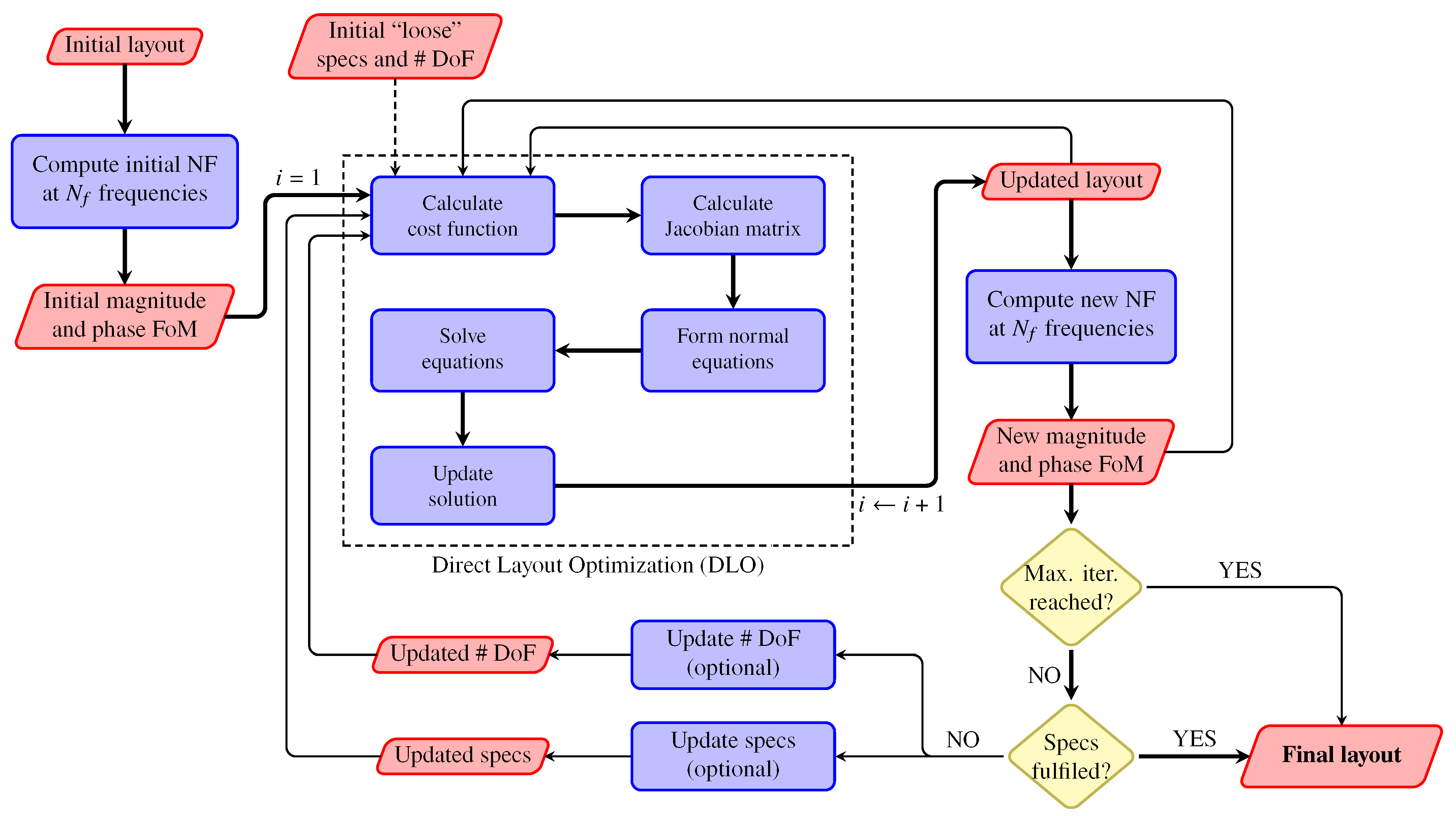
2.2. Direct Layout Optimization Algorithm

Once the relevant FoM have been established, they may be employed in a general NF synthesis consisting of the direct layout optimization (DLO) of the reflectarray. Figure 2 shows the proposed synthesis algorithm. It is based on a gradient-based algorithm, namely, the Levenberg–Marquard (LM) algorithm [38], to perform the DLO.

2.2.1. Inputs of the Algorithm

The algorithm has several inputs that are required to correctly perform the optimization: a starting layout of the reflectarray with the sizes of the geometrical features of the chosen unit cell (for instance, the dimensions of rectangular patches, the lengths of dipoles, etc.), the FoM specifications, the actual FoM calculated from the NF, and the number of degrees of freedom (DoF) which are going to be optimized.

We consider a unit cell with L geometrical features. Since the reflectarray has N elements, the total number of available DoF for optimization is $P=LN$. Thus, we can consider the vector $\overrightarrow{\xi }=\{{\xi }_1,{\xi }_2,\dots ,{\xi }_p,\dots ,{\xi }_P\}$ as representing the reflectarray layout, where ${\xi }_p$ represents a DoF. In general, the total number of available DoF may be relatively large. For instance, some multi-resonant unit cells may have up to eight [39] DoF per element. If the reflectarray has several thousands of elements [40], then, the total number of DoF can be in the range of several tens of thousands of DoF. Some specific applications, such as high resolution SAR, may require optimization of more than 160,000 variables [41]. This may create difficulties in achieving successful optimization since the number of local minima grow exponentially with the number of DoF. To tackle this issue, one common approach is to start the optimization with a reduced number of DoF and loose requirements and gradually increase the number of DoF, while tightening the restrictions until convergence is achieved, as illustrated in the flowchart in Figure 2.

Another input is the FoM calculated from the NF. In the present investigation, and for the purposes of optimizing a reflectarray to work as a PWG, we consider the magnitude and phase ripple as defined in (5) and (6), respectively. Thus, the total number of FoM to consider in the synthesis is two per frequency and polarization. Since there are $N_f$ frequencies and the reflectarray will work in dual-linear polarization, there will be $4N_f$ FoM to optimize. Similarly, the specifications that are also an input to the algorithm will impose the desired values that the FoM need to achieve.

2.2.2. Multi-Frequency Direct Layout Optimization

The proposed multi-frequency DLO consists of an iterative procedure. Starting with the initial layout, given by the values contained in vector $\overrightarrow{\xi }$, the NF generated by the reflectarray is calculated at a number of frequencies. From this NF, the initial magnitude and phase FoM are calculated for each orthogonal polarization and frequency. The next step is to calculate the cost function. To this end, three elements are needed: the value of the current FoM (${\Delta }_{k,{\mathsf{\Omega }}_m}^{m/p}$), the specifications that are to be met (${\tilde{\Delta }}_{k,{\mathsf{\Omega }}_m}^{m/p}$), and the weight functions to leverage the error of each FoM (W). Then, the cost function is defined as:

$$r_{f,k,m}=W_{f,k,m}\left({\tilde{\Delta }}_{k,{\mathsf{\Omega }}_m}^{m/p}-{\Delta }_{k,{\mathsf{\Omega }}_m}^{m/p}\right),$$

(7)

where $f=1,2,\dots ,N_f$ is the index for the dependence on the frequency, with $N_f$ the total number of frequencies at which the optimization is carried out; $k=1,2,\dots ,K$ is the index for the number of FoM (K in total) defined in region ${\mathsf{\Omega }}_m$; and $m=1,2,\dots ,M$ is the index for the different regions where FoM may be defined. Please note that it is not necessary to optimize FoM in all regions. Since the LM algorithm is employed, the cost function defined in (7) is also known as the residual [38].

The next step is to compute the Jacobian matrix. The size of this matrix depends on the total number of DoF taken into account in the current iteration (which may vary from one to another) and the total number of FoM that are optimized. The number of DoF define the number of columns, while the number of FoM define the number of rows. Thus, the size of the matrix is $4N_f\times N_P$, where $N_P\le P=LN$. Any element of the Jacobian matrix may be calculated as:

$$J(q,s)={\displaystyle \frac{\partial r_q}{\partial {\xi }_s}},$$

(8)

where $q=1,2,\dots ,4N_f$, and $s=1,2,\dots ,N_P$. In (8), the dependence on indices f, k and m has been dropped to alleviate the notation. In addition, although not directly specified, the residual depends on the optimizing variables since $\overrightarrow{\xi }$ defines the electromagnetic response of the reflectarray unit cell that will shape the NF from which the FoM are calculated to obtain the residual. In addition, the partial derivative in (8) may be numerically evaluated by means of finite differences [38,42], that, for the particular case of gradient-based algorithms for array antenna synthesis, can be efficiently computed using the differential contributions technique [43].

Once the Jacobian matrix has been computed, the normal equations are formed:

$$\left[J_i^T{J}_i+{\mu }_i\mathrm{diag}\left(J_i^T{J}_i\right)\right]{\delta }_i=-J_i^T{r}_i,$$

(9)

which can be compactly written as:

$$A_i{\delta }_i=b_i,$$

(10)

where subindex i denotes the current iteration (see Figure 2), $J^T$ is the transpose of the Jacobian matrix, $\mu$ is a real positive number, $\mathrm{diag}(·)$ is the diagonal matrix, and ${\delta }_i$ is the updating vector that satisfies the equality. Since matrix $A_i$ is at least semi-positive definite, an efficient Cholesky factorization can be used to solve (10) for ${\delta }_i$.

After the normal equations are solved, the solution is updated as:

$${\overrightarrow{\xi }}_{i+1}={\overrightarrow{\xi }}_i+{\delta }_i.$$

(11)

With the updated layout ${\overrightarrow{\xi }}_{i+1}$, the NF and FoM are computed again and checked against the specifications. If the requirements are met, the algorithm stops and ${\overrightarrow{\xi }}_{i+1}$ is the final layout. Otherwise, the number of DoF in the optimization may be modified, as well as the specifications, and the process is repeated again until convergence or a given maximum number of iterations is reached.

3. Application to Reflectarray for Compact Antenna Test Range

The algorithm proposed in the previous section will now be applied to the optimization of a reflectarray array for its use as a probe in a CATR.

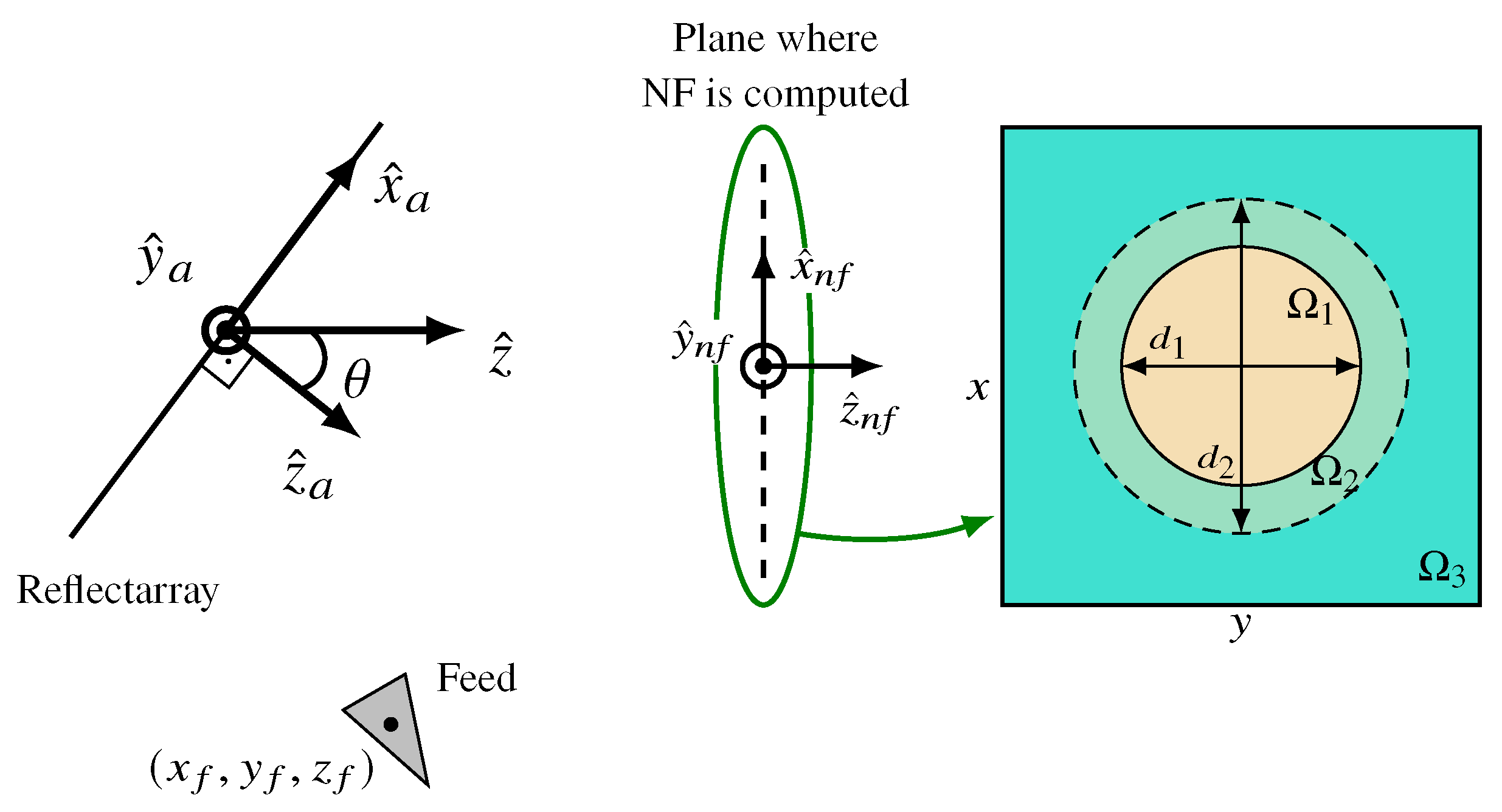
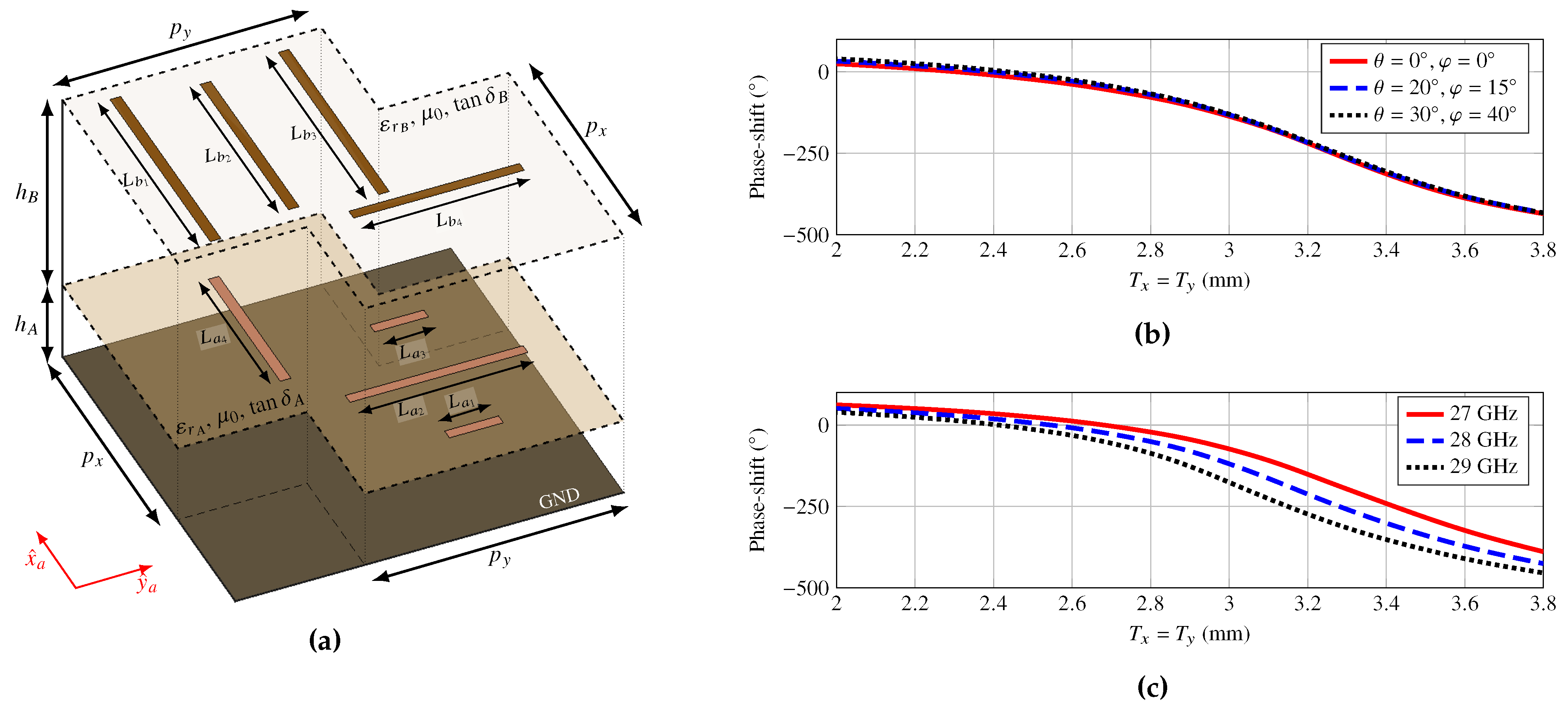
3.1. Antenna Definition, Near-Field Specifications and Unit Cell Characterization

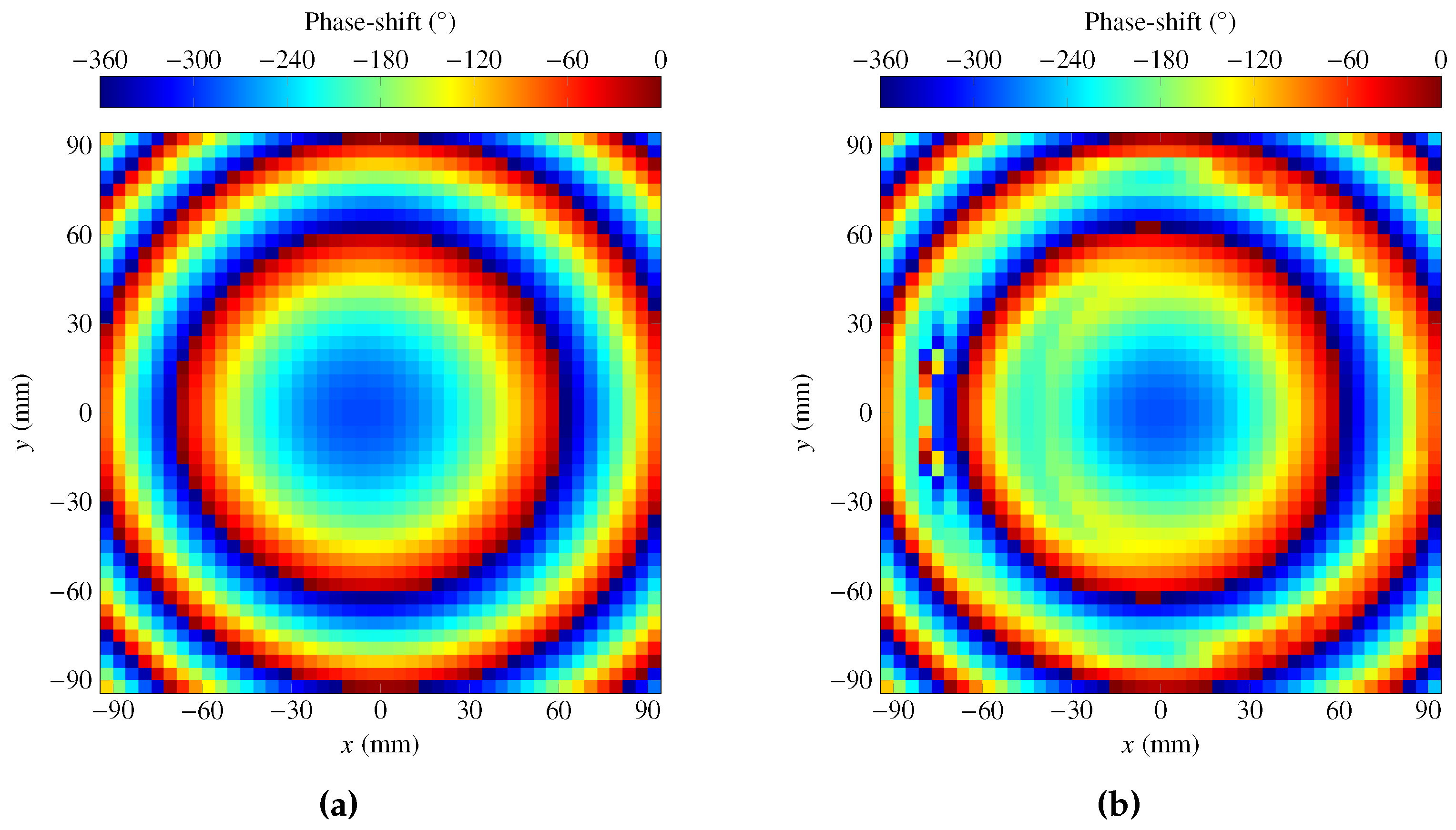
A square reflectarray comprised of $N=1936$ elements distributed in a regular grid of $44\times 44$ unit cells is chosen. The periodicity is $p_x=p_y=4.29\mathrm{mm}$ in both directions, which is approximately $0.4\lambda$ at 28 GHz. The phase center of the feed is placed at ${\overrightarrow{r}}_f=(-79.3,0,200)\mathrm{mm}$ with regard to the reflectarray center (see Figure 1). The feed generates an illumination taper that varies between $-15.4\mathrm{dB}$ at 27 GHz and $-16.3\mathrm{dB}$ at 29 GHz.

The goal is to design a reflectarray that acts as a probe in a CATR system, where an antenna or device under test is placed in the region where a plane wave is generated in front of the antenna. The reflectarray feed would emit a wave, which is transformed into a plane wave by the reflectarray and is then collected by the device being measured. Thus, regarding specifications, the goal is to shape the near field in a plane in front of the reflectarray in such a way that it complies with a maximum magnitude ripple of 1 dB and a maximum phase ripple of 10°.

To this end, these FoM are computed in a tilted plane (see Figure 3) at $z=0.5\mathrm{m}$ (in the ACS), whose rotation is defined by $\theta =20°,\phi =0°,\psi =0°$ (see Appendix in [24]). The region is subsequently divided into three subregions: ${\mathsf{\Omega }}_1$ where the FoM are calculated, ${\mathsf{\Omega }}_2$ which defines a transition, and ${\mathsf{\Omega }}_3$ which comprises the rest of the plane. Although regions ${\mathsf{\Omega }}_2$ and ${\mathsf{\Omega }}_3$ are not used for this particular optimization, they will become relevant when comparing the new proposed technique with others described in the literature in Section 3.4. In addition, regions ${\mathsf{\Omega }}_1$ and ${\mathsf{\Omega }}_2$ are circles with diameter $d_1=100\mathrm{mm}$ and $d_2=200\mathrm{mm}$, respectively.

The chosen unit cell is depicted in Figure 4a. It consists of two layers of parallel and coplanar dipoles, arranged such that each set of four dipoles control the phase-shift for one linear polarization. The substrate has a thickness of $h_A=h_B=0.787\mathrm{mm}$, a relative permittivity of ${\epsilon }_A={\epsilon }_B=2.33$ and a loss tangent of $\tan {\delta }_A=\tan {\delta }_B=0.0013$. The separation center-to-center between parallel dipoles is 0.9 mm and the dipole width is 0.4 mm. This unit cell provides up to eight DoF for optimization purposes (the dipole lengths). However, to analyse the electromagnetic response of the unit cell and to obtain the initial layout (see Section 3.2), two variables are defined, $T_x$ and $T_y$, that are related to the dipole lengths as follows:

$$\begin{array}{cc}\hfill L_{a_1}& =0.5T_y;L_{a_2}=T_y;L_{a_3}=0.5T_y;L_{a_4}=T_x\hfill \\ \hfill L_{b_1}& =0.5T_x;L_{b_2}=0.9T_x;L_{b_3}=0.5T_x;L_{b_4}=0.93T_y.\hfill \end{array}$$

(12)

These scaling factors were determined after carrying out a parametric study to obtain a smooth variation of the phase-shift for $T_x=T_y$ at several frequencies and angles of incidence. Figure 4b shows the phase-shift at 28 GHz for several angles of incidence. As can be seen, the electromagnetic response of the unit cell presents good angular stability while providing a phase-shift larger than 360°, making it suitable for reflectarray design and optimization [35]. On the other hand, Figure 4c shows the phase-shift response for oblique incidence with $(\theta =40°,\phi =30°)$ at three frequencies belonging to the fifth generation new radio (5G NR) n257 band. In all cases, the phase-shift range is larger than 400°, making it suitable also for multi-frequency optimization.

3.2. Initial Layout

The multi-frequency DLO requires an initial reflectarray layout that must be generated prior to the use of the technique. Here, the layout is obtained following a multi-step procedure [44] in which, first, a phase-only synthesis (POS) at 28 GHz is carried out to obtain a phase-shift distribution such that it radiates the desired NF at the frequency of synthesis. To this end, the generalized intersection approach (GIA) [45] particularized for a reflectarray NF model [24] is employed. For the POS, the initial phase-shift distribution shown in Figure 5a was used. It corresponds to a far field-focused reflectarray pointing at $\theta =20°$ (see Figure 3). After the POS with the GIA, the phase-shift distribution of Figure 5b was obtained.

Then, the lengths of the dipoles are adjusted element-by-element so that they provide the required phase-shift obtained after the POS. For this process, variables $T_x$ and $T_y$ defined in (12) are employed, such that $T_x$ controls the phase-shift for linear polarization X and $T_y$ for polarization Y. Figure 6 shows a comparison of the NF before and after the POS at 28 GHz for polarization X. As can be seen, even though the field does not fully comply with the imposed specifications, it greatly improves when compared with the starting point before the POS. Indeed, the magnitude ripple is reduced from a maximum of 7.6 dB before the POS to a maximum of 2.2 dB after the POS. For the phase, the maximum ripple was reduced from 26.4° to 13.6°.

The POS enables obtaining a layout that works relatively well at the frequency of design, 28 GHz in this case. However, performance rapidly deteriorates as the frequency is shifted. This can be seen in

Table 1. Performance of the reflectarray before and after the POS with the GIA at a plane 0.5 m away from the antenna. After the POS, the layout is simulated at three different frequencies within the 5G FR n257 band to assess the performance. Before POS, results are only shown at 28 GHz since ideal phase-shifters are assumed. Compliance (%) indicates percentage of surface in ${\mathsf{\Omega }}_1$ that complies with specifications.

Reflectarray	Frequency (GHz)	Compliance (%)						Ripple
		Pol. X			Pol. Y			Pol. X			Pol. Y
		Mag.	Phase		Mag.	Phase		Mag. (dB)	Phase (°)		Mag. (dB)	Phase (°)
Before POS	28 GHz	25.51	49.79		26.75	57.00		7.57	26.35		6.61	20.95
After POS	27 GHz	81.69	76.34		66.77	63.89		1.56	20.91		1.86	24.12
	28 GHz	60.60	97.84		69.24	96.40		1.80	11.51		2.16	13.59
	29 GHz	39.77	89.51		36.93	50.31		3.17	15.43		5.02	22.86

, which gathers information concerning the compliance according to the imposed specifications (maximum ripple in magnitude of 1 dB and in phase of 10°), as well as the maximum ripple in magnitude and phase. As can be seen, even though the magnitude ripple decreases slightly at 27 GHz compared to the central frequency, the phase ripple increases considerably. In addition, both magnitude and phase ripples deteriorate considerably at the upper frequency of 29 GHz, indicating that a wideband multi-frequency optimization is needed.

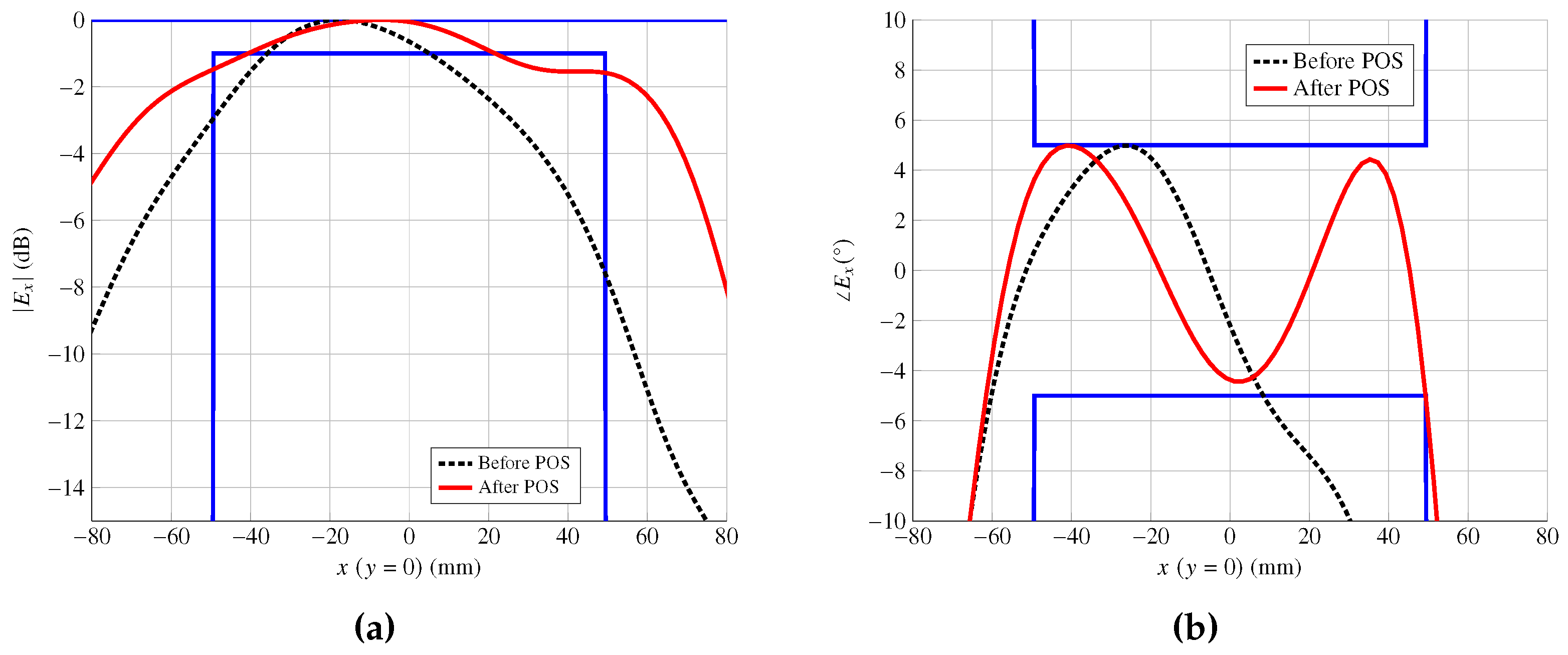
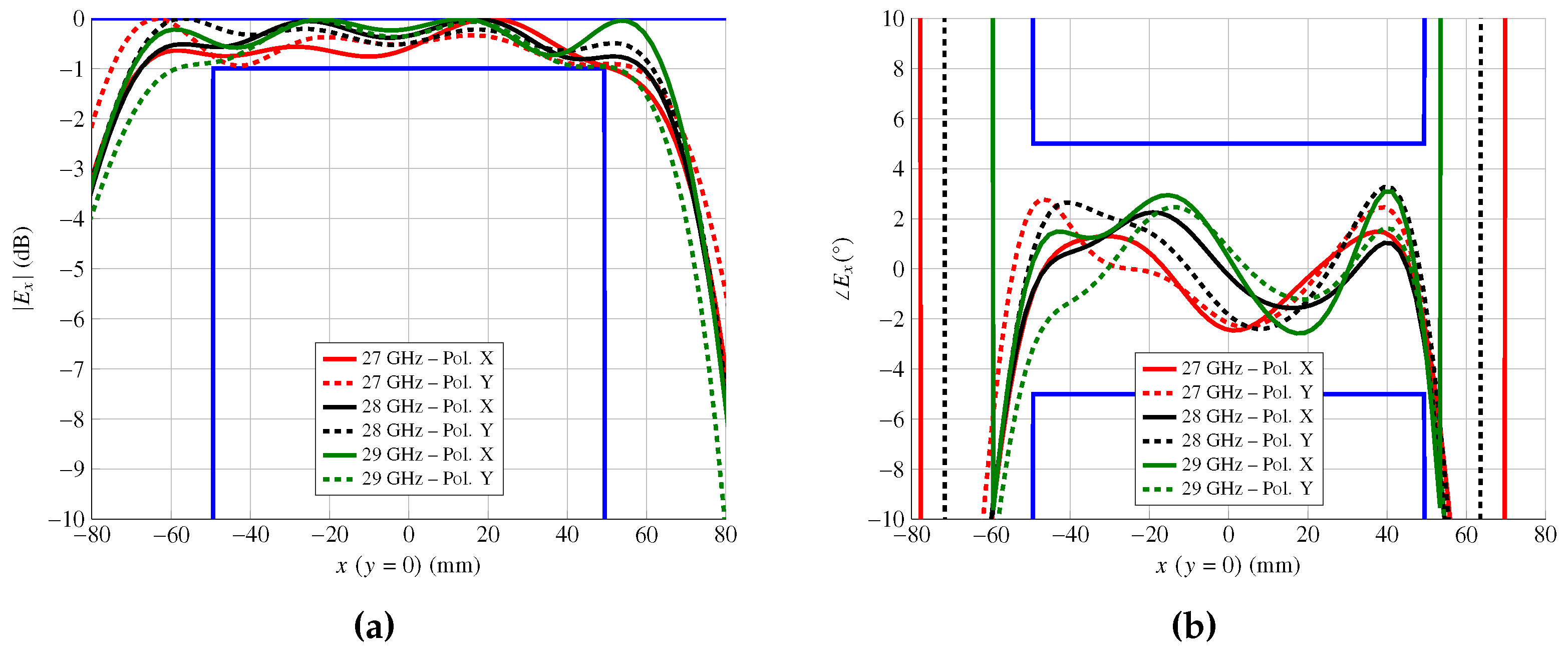
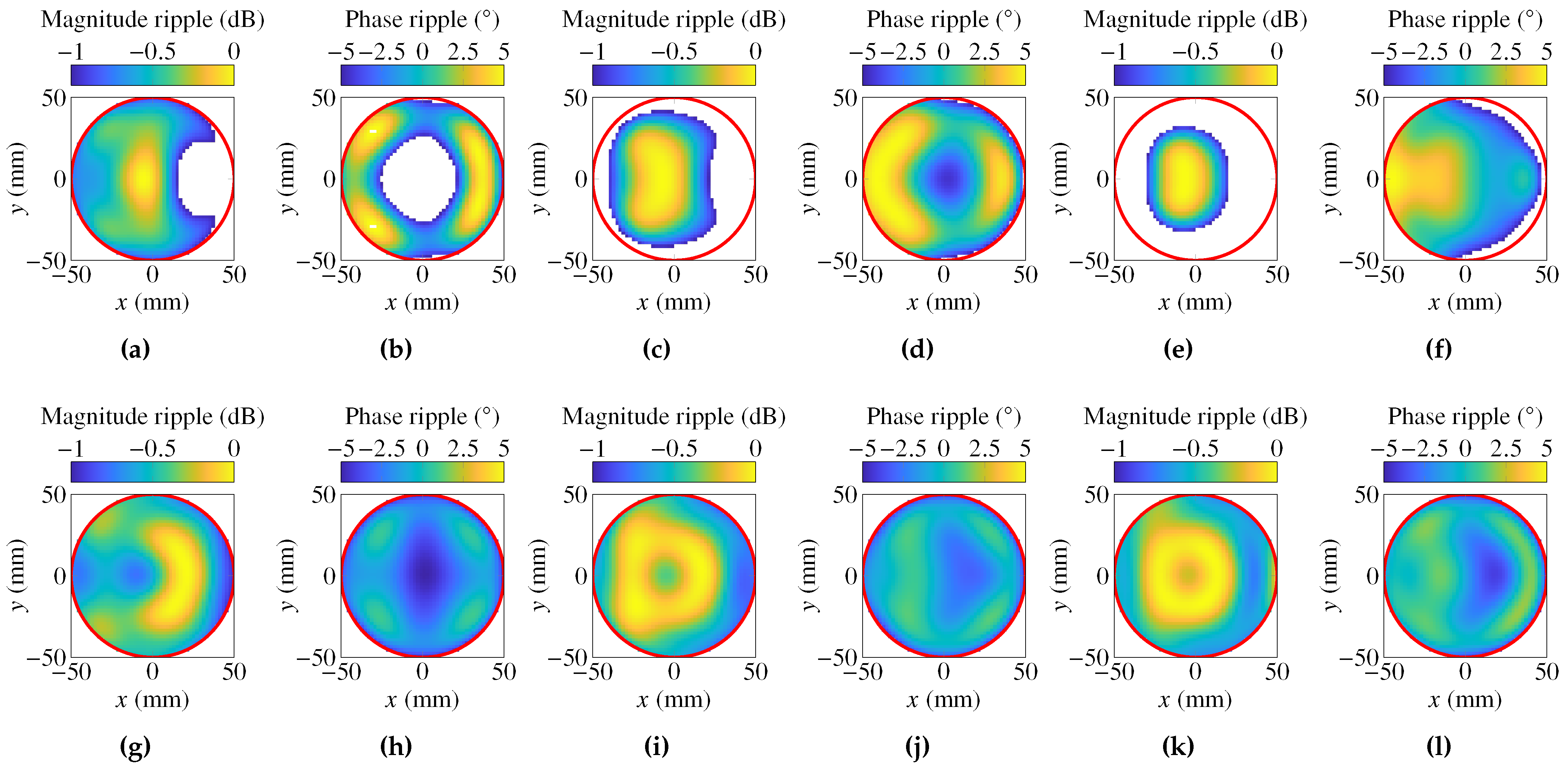
3.3. Wideband Multi-Frequency Optimization of the Near-Field Figures of Merit

The next step is to carry out a multi-frequency optimization of the reflectarray layout to improve performance in the frequency range of interest. To this end, the multi-frequency optimization algorithm of Figure 2 is employed. The synthesis is carried out at three frequencies within the 5G FR n257 band, 27 GHz, 28 GHz and 29 GHz. In addition, two linear polarizations are optimized, considering requirements in both magnitude and phase ripples. Thus, a total of 12 FoM are optimized. In order to ease the optimization and facilitate convergence towards a solution, a multi-stage procedure is adopted [46]. A total of six stages are considered: first, only the dipoles oriented in the ${\widehat{x}}_a$ direction are optimized by means of the $T_x$ variable. In the second stage, only the dipoles oriented in the ${\widehat{y}}_a$ are optimized by means of the $T_y$ variable. Then, in the third stage, both variables $T_x$ and $T_y$ are optimized at the same time for all reflectarray unit cells.

For the last three stages, a similar procedure is followed, but increasing the number of DoF per reflectarray element. Now, the DoFs are the lengths of all dipoles but maintaining the cell symmetry with $L_{a_1}=L_{a_3}$ and $L_{b_1}=L_{b_3}$ (see Figure 4a), i.e., $T_{x_1}=L_{b_1}=L_{b_3}$, $T_{x_2}=L_{b_2}$, $T_{x_3}=L_{a_4}$, $T_{y_1}=L_{a_1}=L_{a_3}$, $T_{y_2}=L_{a_2}$, $T_{y_3}=L_{b_4}$. The new variables are $T_{x_i}$ and $T_{y_i}$, $i=1,2,3$, for each reflectarray element. Thus, in the fourth stage, only variables $T_{x_1}$, $T_{x_2}$ and $T_{x_3}$ are considered, while, in the fifth stage, the optimizing variables are $T_{y_1}$, $T_{y_2}$ and $T_{y_3}$. Finally, in the sixth and last stage, all six variables per element are optimized.

By following this procedure with the algorithm of Figure 2, and imposing requirements of a maximum magnitude ripple of 1 dB and a maximum phase ripple of 10° for both linear polarizations and three frequencies, the results of Figure 7 are obtained. The main cut ($y=0\mathrm{mm}$) is shown for both linear polarizations at the three considered frequencies for magnitude and phase. Now, the magnitude and phase fully comply with the requirements of a plane wave inside region ${\mathsf{\Omega }}_1$ where the FoM are defined (see Figure 3).

The improvement in compliance of the QZ is better seen in Figure 8. This represents, for linear polarization X at the three frequencies of interest, the magnitude and phase in region ${\mathsf{\Omega }}_1$ that complies with the requirements of a plane wave before and after the multi-frequency optimization. The starting layout does not fully comply with specifications at any of the frequencies, although at the central frequency the phase almost does, as also shown in Table 1. After the optimization, the requirements are met for both magnitude and phase at the three frequencies for which the FoM were optimized.

Table 2. Performance of the reflectarray after the wideband multi-frequency optimization at a plane 0.5 m away from the antenna. Compliance (%) indicates percentage of surface in ${\mathsf{\Omega }}_1$ that complies with specifications.

Frequency (GHz)	Compliance (%)						Ripple
	Pol. X			Pol. Y			Pol. X			Pol. Y
	Mag.	Phase		Mag.	Phase		Mag. (dB)	Phase (°)		Mag. (dB)	Phase (°)
27 GHz	100	100		100	100		0.98	5.81		0.77	5.52
28 GHz	100	100		100	100		0.86	6.13		0.54	6.51
29 GHz	100	100		100	100		0.75	6.87		0.98	6.39

gathers the performance data of the optimized antenna. A compliance of 100% in region ${\mathsf{\Omega }}_1$ (see Figure 3) is achieved. Compared with the initial layout obtained after the POS, the worst magnitude ripple was reduced from 5.02 dB to 0.98 dB, while the worst phase ripple was reduced from 24.12° to 6.87°.

3.4. Comparison with Other Techniques in the Literature

Table 3. Comparison of the proposed algorithm with other techniques described in the literature in terms of type of constraints, capabilities and computational performance.

Reference	Constraint Type	Magnitude Constraints	Phase Constraints	Multi-Frequency Optimization	Memory Footprint	Computational Efficiency
[28]	Upper & lower templates	Yes	Yes	No	High	Medium
[32]	Upper & lower templates	Yes	No	No	High	Medium
[33]	Upper & lower templates	Yes	No	No	Low	High
[34]	Upper & lower templates	Yes	No	No	High	Medium
This work	Relevant figures of merit	Yes	Yes	Yes	Low	Medium

shows a comparison of the proposed optimization technique for spatially fed arrays with others described in the literature in terms of the type of constraints, capabilities and computational performance. The other techniques are based on the definition of upper and lower templates in the region of interest that are used to trim the near field according to the given specifications [47]. Although it is claimed that figures of merit, such as pointing direction, ripple, secondary lobes, etc., are optimized [33], in reality, they are used to define the templates which are the ones actually used in the algorithm. This is true for the studies cited in Table 3. Only the present study directly optimizes the relevant figures of merit, as described in previous sections. In addition, all techniques implement at least NF magnitude constraints, although this is not the case for phase constraints that are necessary for applications such as PWG for CATR. However, it would be possible to extend the techniques with proper definition of upper and lower phase templates.

In the area of NF-field-shaping for spatially fed arrays, the present study is the first in which a multi-frequency optimization with both magnitude and phase constraints is implemented, which enables a wideband array to be obtained when performance would otherwise deteriorate at frequencies different from the designated frequency.

A more direct comparison can be performed with the synthesis technique employed in [28], since it also implements both magnitude and phase constraints. To this end, upper and lower templates [47] were defined in three regions, ${\mathsf{\Omega }}_1$, ${\mathsf{\Omega }}_2$ and ${\mathsf{\Omega }}_3$, as shown in Figure 3. ${\mathsf{\Omega }}_1$ is still the region where the plane wave is to be generated and so the templates impose ripples of 1 dB for the magnitude and 10° for the phase. ${\mathsf{\Omega }}_2$ defines a transition zone only for the magnitude, while ${\mathsf{\Omega }}_3$ is the non-coverage area. To ease the optimization, a maximum side-lobe level of $-10\mathrm{dB}$ is imposed. In the case of the phase, in regions ${\mathsf{\Omega }}_2$ and ${\mathsf{\Omega }}_3$, no constraints are specified. The same procedure described in Section 3.3 is applied, increasing the number of optimizing variables in six successive stages, but, this time, considering the upper and lower templates instead of the relevant figures of merit. By following this strategy, the results shown in

Table 4. Performance of the reflectarray after wideband multi-frequency optimization at a plane 0.5 m away from the antenna employing a multi-frequency version of the technique used in [28] with specifications imposed by upper and lower templates. Compliance (%) indicates percentage of surface in ${\mathsf{\Omega }}_1$ that complies with specifications.

Frequency (GHz)	Compliance (%)						Ripple
	Pol. X			Pol. Y			Pol. X			Pol. Y
	Mag.	Phase		Mag.	Phase		Mag. (dB)	Phase (°)		Mag. (dB)	Phase (°)
27 GHz	97.16	96.53		100	94.01		1.19	11.31		0.94	11.63
28 GHz	90.85	99.68		91.17	96.53		1.39	10.19		1.35	10.94
29 GHz	66.88	94.01		63.41	92.43		1.93	11.18		2.48	11.46

were obtained. Although these certainly indicate a net improvement over the starting point of Table 1 (all compliances increase, all maximum ripples decrease), the results do not fully comply with the imposed specifications. However, as shown earlier, when directly optimizing the relevant FoM, a 100% compliance is achieved in dual-linear polarization at three different frequencies. Moreover, to achieve the results shown in Table 4 a total of 700 iterations of the algorithm were necessary across all six stages, but only 187 iterations were needed to obtain the results shown in Table 2. This is consistent with the results shown for far-field synthesis [48], where directly optimizing the FoM provided better results in fewer iterations than using upper and lower templates.

Regarding computational efficiency, directly optimizing the FoM also offers advantages over using upper and lower templates. The present study, as well as others [28,32,34], employed the LM algorithm to minimize a cost function at some point in the optimization procedure. This algorithm requires the computation of a Jacobian matrix (see Figure 2), which is a data structure that takes more memory to store. In the present investigation, the maximum size of the Jacobian matrix is $4N_f\times LN$, where $N_f$ is the number of frequencies, L is the number of geometrical features of the unit cell that are being optimized, and N is the total number of reflectarray elements. For the example considered here, $N_f=3$, $L=2\mathrm{or}6$, and $N=1936$. Thus, the maximum size would be 2.13 MB, assuming double-precision complex numbers. If upper and lower mask templates are employed, the size of the Jacobian considerably increases, since, now, all points into which region $\mathsf{\Omega }$ is discretized are stored per frequency in the Jacobian matrix. In the present case, region $\mathsf{\Omega }$ was discretized in a grid of $150\times 150$ points. Thus, the size of the Jacobian in that case is 11.68 GB. Thus, by optimizing the FoM the size of the Jacobian matrix is reduced by more than three orders of magnitude. If more than one NF plane was optimized, the size of the Jacobian would further increase. In this case, the memory footprint could be alleviated to some extent by reducing the number of points where the NF is calculated. For instance, in [43] an NF grid of $81\times 81$ points is employed. In this case, the size of the Jacobian would be 3.4 GB, which is still more than three orders of magnitude larger than when directly optimizing FoM.

4. Conclusions

In this paper, a new general near-field (NF) multi-frequency optimization technique has been presented. It relies on the proper definition of the magnitude and phase figures of merit (FoM) to be optimized in the region of interest. By employing a full-wave technique based on local periodicity, the full electromagnetic response of the reflectarray unit cell is obtained at a number of frequencies where the NF and the associated FoM are calculated. Then, by applying an iterative multi-stage procedure based on the Levenberg–Marquardt algorithm, a direct layout optimization is carried out. This procedure was applied to obtain a reflectarray that acts as a plane-wave generator for a compact antenna test range within the 5G FR n257 band. Typical plane-wave specifications of a maximum magnitude ripple of 1 dB and a phase ripple of 10° were imposed. The optimized reflectarray fully complies with the imposed requirements in a frequency range between 27 GHz and 29 GHz, corresponding to a relative bandwidth of 7.14%.

Compared with other techniques described in the literature for the NF-beam-shaping of spatially fed arrays, the proposed technique is able to carry out a general NF multi-frequency optimization, while other techniques only perform the synthesis at a single frequency. In addition, due to the direct optimization of the relevant FoM instead of relying on the use of upper and lower templates, better results are achieved in fewer iterations, demonstrating superior computational performance. Moreover, the memory footprint is also greatly reduced compared with other techniques described in the literature.

References

1. 3GPP. Technical Specification Group Radio Access Network; NR; User Equipment (UE) Radio Transmission and Reception; Part 2: Range 2 Standalone (Release 17). Technical Report, 3GPP, Sophia Antipolis, France. 2022. Available online: https://www.3gpp.org/ftp/Specs/archive/38_series/38.101-2/ (accessed on 17 November 2022).
2. Wijethilaka, S.; Liyanage, M. Survey on Network Slicing for Internet of Things Realization in 5G Networks. IEEE Commun. Surv. Tutor. 2021, 23, 957–994. [Google Scholar] [CrossRef]
3. Lin, Z.; Lin, M.; de Cola, T.; Wang, J.B.; Zhu, W.P.; Cheng, J. Supporting IoT with Rate-Splitting Multiple Access in Satellite and Aerial-Integrated Networks. IEEE Internet Things J. 2021, 8, 11123–11134. [Google Scholar] [CrossRef]
4. Gohar, A.; Nencioni, G. The Role of 5G Technologies in a Smart City: The Case for Intelligent Transportation System. Sustainability 2021, 13, 5188. [Google Scholar] [CrossRef]
5. Attaran, M. The impact of 5G on the evolution of intelligent automation and industry digitization. J. Ambient Intell. Humaniz. Comput. 2021. [Google Scholar] [CrossRef]
6. Szalay, Z.; Ficzere, D.; Tihanyi, V.; Magyar, F.; Soós, G.; Varga, P. 5G-Enabled Autonomous Driving Demonstration with a V2X Scenario-in-the-Loop Approach. Sensors 2020, 20, 7344. [Google Scholar] [CrossRef]
7. Lin, Z.; Niu, H.; An, K.; Wang, Y.; Zheng, G.; Chatzinotas, S.; Hu, Y. Refracting RIS-Aided Hybrid Satellite-Terrestrial Relay Networks: Joint Beamforming Design and Optimization. IEEE Trans. Aerosp. Electron. Syst. 2022, 58, 3717–3724. [Google Scholar] [CrossRef]
8. Lin, Z.; An, K.; Niu, H.; Hu, Y.; Chatzinotas, S.; Zheng, G.; Wang, J. SLNR-based Secure Energy Efficient Beamforming in Multibeam Satellite Systems. IEEE Trans. Aerosp. Electron. Syst. 2022; 1–4, early access. [Google Scholar] [CrossRef]
9. Lin, Z.; Lin, M.; Wang, J.B.; de Cola, T.; Wang, J. Joint Beamforming and Power Allocation for Satellite-Terrestrial Integrated Networks With Non-Orthogonal Multiple Access. IEEE J. Sel. Top. Signal Process. 2019, 13, 657–670. [Google Scholar] [CrossRef] [Green Version]
10. Rischke, J.; Sossalla, P.; Itting, S.; Fitzek, F.H.P.; Reisslein, M. 5G Campus Networks: A First Measurement Study. IEEE Access 2021, 9, 121786–121803. [Google Scholar] [CrossRef]
11. Hong, W.; Jiang, Z.H.; Yu, C.; Hou, D.; Wang, H.; Guo, C.; Hu, Y.; Kuai, L.; Yu, Y.; Jiang, Z.; et al. The Role of Millimeter-Wave Technologies in 5G/6G Wireless Communications. IEEE J. Microw. 2021, 1, 101–122. [Google Scholar] [CrossRef]
12. Rappaport, T.S.; Sun, S.; Mayzus, R.; Zhao, H.; Azar, Y.; Wang, K.; Wong, G.N.; Schulz, J.K.; Samimi, M.; Gutierrez, F. Millimeter Wave Mobile Communications for 5G Cellular: It Will Work! IEEE Access 2013, 1, 335–349. [Google Scholar] [CrossRef]
13. Álvarez-Narciandi, G.; Laviada, J.; Las-Heras, F. Last advances in freehand sensing for mmWave imaging. In Proceedings of the IEEE International Symposium on Antennas and Propagation (AP-S), Denver, CO, USA, 10–15 July 2022; pp. 734–735. [Google Scholar] [CrossRef]
14. López, Y.A.; García-Fernández, M.; Las-Heras, F. A Portable Cost-Effective Amplitude and Phase Antenna Measurement System. IEEE Trans. Instrum. Meas. 2020, 69, 7240–7251. [Google Scholar] [CrossRef]
15. Álvarez-Narciandi, G.; Laviada, J.; Álvarez-López, Y.; Ducournau, G.; Luxey, C.; Belem-Goncalves, C.; Gianesello, F.; Nachabe, N.; Rio, C.D.; Las-Heras, F. Freehand System for Antenna Diagnosis Based on Amplitude-Only Data. IEEE Trans. Antennas Propag. 2021, 69, 4988–4998. [Google Scholar] [CrossRef]
16. Olver, A.D. Compact antenna test ranges. In Proceedings of the Seventh International Conference on Antennas and Propagation (ICAP), York, UK, 15–18 April 1991; pp. 99–108. [Google Scholar]
17. Chang, D.C.; Yang, S.Y.; Ho, M.R. Compact range design with axial-symmetric main reflector. In Proceedings of the Proc. Antennas and Propagation Society International Symposium, San Jose, CA, USA, 26–30 June 1989; pp. 328–331. [Google Scholar] [CrossRef]
18. Mompó, R.; Molina, J.; Calvo, M.; Besada, J.L. Compact range antenna analysis. In Proceedings of the Electrotechnical Conference Integrating Research, Industry and Education in Energy and Communication Engineering, Lisbon, Portugal, 11–13 April 1989; pp. 497–500. [Google Scholar] [CrossRef]
19. Wong, K.T.; Excell, P.S. A compact range fed by an array of log-periodic dipole antennas. In Proceedings of the IEE Colloquium on Advances in the Direct Measurement of Antenna Radiation Characteristics in Indoor Environments, London, UK, 23 January 1989; pp. 1–4. [Google Scholar]
20. Jackson, N.N.; Excell, P.S. A compact range using and array antenna. In Proceedings of the IEE Colloquium on Radiated Emission Test Facilities, London, UK, 2 June 1992; pp. 1–5. [Google Scholar]
21. Iupikov, O.A.; Krasov, P.S.; Glazunov, A.A.; Maaskant, R.; Fridén, J.; Ivashina, M.V. Hybrid OTA Chamber for Multidirectional Testing of Wireless Devices: Plane Wave Spectrum Generator Design and Experimental Demonstration. IEEE Trans. Antennas Propag. 2022, 70, 10974–10987. [Google Scholar] [CrossRef]
22. Zhang, Y.; Wang, Z.; Ren, Y.; Pan, C.; Zhang, J.; Jia, L.; Zhu, X. A Novel Metasurface Lens Design for Synthesizing Plane Waves in Millimeter-Wave Bands. Electronics 2022, 11, 1403. [Google Scholar] [CrossRef]
23. Pietrenko-Dabrowska, A.; Koziel, S. Low-Cost Design Optimization of Microwave Passives Using Multifidelity EM Simulations and Selective Broyden Updates. IEEE Trans. Microw. Theory Tech. 2022, 70, 4765–4771. [Google Scholar] [CrossRef]
24. Prado, D.R. Near Field Models of Spatially-Fed Planar Arrays and Their Application to Multi-Frequency Direct Layout Optimization for mm-Wave 5G New Radio Indoor Network Coverage. Sensors 2022, 22, 8925. [Google Scholar] [CrossRef]
25. Encinar, J.A. Design of two-layer printed reflectarrays using patches of variable size. IEEE Trans. Antennas Propag. 2001, 49, 1403–1410. [Google Scholar] [CrossRef]
26. Pozar, D.M.; Targonski, S.D.; Syrigos, H.D. Design of millimeter wave microstrip reflectarrays. IEEE Trans. Antennas Propag. 1997, 45, 287–296. [Google Scholar] [CrossRef]
27. Prado, D.R.; Arrebola, M.; Pino, M.R.; Las-Heras, F. Evaluation of the quiet zone generated by a reflectarray antenna. In Proceedings of the International Conference on Electromagnetics in Advanced Applications (ICEAA), Cape Town, South Africa, 2–7 September 2012; pp. 702–705. [Google Scholar] [CrossRef]
28. Vaquero, A.F.; Arrebola, M.; Pino, M.R.; Florencio, R.; Encinar, J.A. Demonstration of a Reflectarray with Near-field Amplitude and Phase Constraints as Compact Antenna Test Range Probe for 5G New Radio Devices. IEEE Trans. Antennas Propag. 2021, 69, 2715–2726. [Google Scholar] [CrossRef]
29. Li, Z.; Huo, P.; Wu, Y.; Wu, J. Reflectarray Compact Antenna Test Range With Controlled Aperture Disturbance Fields. IEEE Antennas Wirel. Propag. Lett. 2021, 20, 1283–1287. [Google Scholar] [CrossRef]
30. Zhao, Y.; Huo, P.; Li, Z. Concept of Transmitarray Compact Antenna Test Range. In Proceedings of the International Conference on Microwave and Millimeter Wave Technology (ICMMT), Nanjing, China, 23–26 May 2021; pp. 1–3. [Google Scholar] [CrossRef]
31. Tang, J.; Chen, X.; Meng, X.; Wang, Z.; Ren, Y.; Pan, C.; Huang, X.; Li, M.; Kishk, A.A. Compact Antenna Test Range Using Very Small F/D Transmitarray Based on Amplitude Modification and Phase Modulation. IEEE Trans. Instrum. Meas. 2022, 71, 1–14. [Google Scholar] [CrossRef]
32. Imaz-Lueje, B.; Vaquero, A.F.; Prado, D.R.; Pino, M.R.; Arrebola, M. Shaped-Pattern Reflectarray Antennas for mm-Wave Networks Using a Simple Cell Topology. IEEE Access 2022, 10, 12580–12591. [Google Scholar] [CrossRef]
33. Loredo, S.; León, G.; Plaza, E.G. A Fast Approach to Near-Field Synthesis of Transmitarrays. IEEE Antennas Wirel. Propag. Lett. 2021, 20, 648–652. [Google Scholar] [CrossRef]
34. Vaquero, A.F.; Pino, M.R.; Arrebola, M. Evaluation of a transmit-array base station for mm-wave communications in the Fresnel region. In Proceedings of the IEEE International Symposium on Antennas and Propagation (AP-S), Denver, CO, USA, 10–15 July 2022; pp. 788–789. [Google Scholar] [CrossRef]
35. Huang, J.; Encinar, J.A. Reflectarray Antennas; John Wiley & Sons: Hoboken, NJ, USA, 2008. [Google Scholar]
36. Stutzman, W.L.; Thiele, G.A. Antenna Theory and Design, 3rd ed.; John Wiley & Sons: Hoboken, NJ, USA, 2012. [Google Scholar]
37. Hirvonen, T.; Ala-Laurinaho, J.P.S.; Tuovinen, J.; Räisänen, A.V. A compact antenna test range based on a hologram. IEEE Trans. Antennas Propag. 1997, 45, 1270–1276. [Google Scholar] [CrossRef]
38. Prado, D.R.; Álvarez, J.; Arrebola, M.; Pino, M.R.; Ayestarán, R.G.; Las-Heras, F. Efficient, accurate and scalable reflectarray phase-only synthesis based on the Levenberg-Marquardt algorithm. Appl. Comput. Electromagn. Soc. J. 2015, 30, 1246–1255. [Google Scholar]
39. Florencio, R.; Encinar, J.A.; Boix, R.R.; Losada, V.; Toso, G. Reflectarray Antennas for Dual Polarization and Broadband Telecom Satellite Applications. IEEE Trans. Antennas Propag. 2015, 63, 1234–1246. [Google Scholar] [CrossRef] [Green Version]
40. Encinar, J.A.; Florencio, R.; Arrebola, M.; Salas-Natera, M.A.; Barba, M.; Page, J.E.; Boix, R.R.; Toso, G. Dual-polarization reflectarray in Ku-band based on two layers of dipole arrays for a transmit-receive satellite antenna with South American coverage. Int. J. Microw. Wirel. Technol. 2018, 10, 149–159. [Google Scholar] [CrossRef] [Green Version]
41. Zhou, M.; Palvig, M.F.; Sørensen, S.B.; de Lasson, J.R.; Alvarez, D.M.; Notter, M.; Schobert, D. Design of Ka-band Reflectarray Antennas for High Resolution SAR Instrument. In Proceedings of the 14th European Conference on Antennas and Propagation (EuCAP), Copenhagen, Denmark, 15–20 March 2020; pp. 1–5. [Google Scholar] [CrossRef]
42. Nocedal, J.; Wright, S.J. Numerical Optimization, 2nd ed.; Springer: New York, NY, USA, 2006. [Google Scholar]
43. Prado, D.R.; Vaquero, A.F.; Arrebola, M.; Pino, M.R.; Las-Heras, F. Acceleration of Gradient-Based Algorithms for Array Antenna Synthesis with Far Field or Near Field Constraints. IEEE Trans. Antennas Propag. 2018, 66, 5239–5248. [Google Scholar] [CrossRef] [Green Version]
44. Prado, D.R.; López-Fernández, J.A.; Arrebola, M.; Pino, M.R.; Goussetis, G. General Framework for the Efficient Optimization of Reflectarray Antennas for Contoured Beam Space Applications. IEEE Access 2018, 6, 72295–72310. [Google Scholar] [CrossRef]
45. Prado, D.R.; Arrebola, M.; Pino, M.R.; Las-Heras, F. Improved Reflectarray Phase-Only Synthesis Using the Generalized Intersection Approach with Dielectric Frame and First Principle of Equivalence. Int. J. Antennas Propag. 2017, 2017, 1–11. [Google Scholar] [CrossRef] [Green Version]
46. Prado, D.R.; Arrebola, M.; Pino, M.R.; Goussetis, G. Broadband Reflectarray with High Polarization Purity for 4K and 8K UHDTV DVB-S2. IEEE Access 2020, 8, 100712–100720. [Google Scholar] [CrossRef]
47. Prado, D.R. The Generalized Intersection Approach for Electromagnetic Array Antenna Beam-Shaping Synthesis: A Review. IEEE Access 2022, 10, 87053–87068. [Google Scholar] [CrossRef]
48. Prado, D.R.; Arrebola, M. Effective XPD and XPI Optimization in Reflectarrays for Satellite Missions. IEEE Antennas Wirel. Propag. Lett. 2018, 17, 1856–1860. [Google Scholar] [CrossRef]
Figure 1. Sketch of the reflectarray configuration for general near-field synthesis based on the optimization of the near-field figures of merit.
Electronics 12 00091 g001
Figure 2. Schematic flowchart of the proposed DLO for a general NF synthesis based on optimization of the relevant NF FoM.
Electronics 12 00091 g002
Figure 3. Schematic representation of the antenna optics. The NF plane is tilted θ = 20 ° with regard to the reflectarray and is divided into three regions. The FoM are defined in region Ω 1 , while region Ω 2 defines a transition and Ω 3 comprises the rest of the plane.
Electronics 12 00091 g003
Figure 4. (a) Sketch of the employed unit cell, consisting of two layers of parallel and coplanar dipoles, arranged in two sets of parallel dipoles to control both linear polarizations independently. (b) Phase response of the unit cell for normal and oblique incidence at 28 GHz, showing that the unit cell response is stable with the angle of incidence. (c) Phase response of the unit cell for three different frequencies for oblique incidence with ( θ = 40 ° , φ = 30 ° ) .
Electronics 12 00091 g004
Figure 5. (a) Initial phase-shift distribution of a far-field-focused reflectarray at 28 GHz. (b) Optimized phase-shift distribution after the POS with the GIA at 28 GHz.
Electronics 12 00091 g005
Figure 6. Near-field comparison before and after the POS with the GIA for the (a) magnitude and (b) phase for the cut y = 0 mm at 28 GHz.
Electronics 12 00091 g006
Figure 7. Main cut y = 0 mm of the near field after the wideband multi-frequency optimization of the layout for the (a) magnitude and (b) phase.
Electronics 12 00091 g007
Figure 8. For linear polarization X, representation of the magnitude and phase of the NF that complies with a magnitude ripple of 1 dB and phase ripple of 10° before (top row) and after (bottom row) the multi-frequency optimization. (a) Magnitude at 27 GHz before optimization. (b) Phase at 27 GHz before optimization. (c) Magnitude at 28 GHz before optimization. (d) Phase at 28 GHz before optimization. (e) Magnitude at 29 GHz before optimization. (f) Phase at 29 GHz before optimization. (g) Magnitude at 27 GHz after optimization. (h) Phase at 27 GHz after optimization. (i) Magnitude at 28 GHz after optimization. (j) Phase at 28 GHz after optimization. (k) Magnitude at 29 GHz after optimization. (l) Phase at 29 GHz after optimization. Similar results were obtained for polarization Y.
Electronics 12 00091 g008