Abstract
The logic dendritic neuron model (LDNM), which is inspired by natural neurons, has emerged as a novel machine learning model in recent years. However, recent studies have also shown that the classification performance of LDNM is restricted by the backpropagation (BP) algorithm. In this study, we attempt to use a heuristic algorithm called the gradient-based optimizer (GBO) to train LDNM. First, we describe the architecture of LDNM. Then, we propose specific neuronal structure pruning mechanisms for simplifying LDNM after training. Later, we show how to apply GBO to train LDNM. Finally, seven datasets are used to determine experimentally whether GBO is a suitable training method for LDNM. To evaluate the performance of the GBO algorithm, the GBO algorithm is compared with the BP algorithm and four other heuristic algorithms. In addition, LDNM trained by the GBO algorithm is also compared with five classifiers. The experimental results show that LDNM trained by the GBO algorithm has good classification performance in terms of several metrics. The results of this study indicate that employing a suitable training method is a good practice for improving the performance of LDNM.
1. Introduction
Neural networks occupy an important position in the field of artificial intelligence. Neurons have important research value as components of neural networks. Since the neuron model was proposed, it has been continuously developed and improved. The first artificial neuron model was proposed by McCulloch and Pitts in 1943. However, this model is too simple and does not take into account the nonlinear mechanism of dendrites [1]. With the development of neurobiology, researchers have discovered the importance of dendritic structures in neural computation [2]. Koch et al. proposed a dendritic neuron model called the cell model [3,4]. However, this model cannot identify the type of synapse and cannot determine which dendrite is needed. This is because the dendritic structure of this model is fixed [5]. Later, Legenstein and Maass also proposed a neuron model with dendritic structures [6]. This model possesses nonlinear computational power but cannot solve problems that are not linearly separable.
The dendritic neuron model, called the logic dendritic neuron model (LDNM), has emerged as a potential machine learning model in recent years. A series of dendritic neuron models have been proposed to address practical problems. Ji et al. proposed a logic dendritic neuron model that has a dendritic structure and can be pruned after training [7]. This model can effectively solve problems that are not linearly separable. Later, Ji et al. focused on the classification ability of LDNM and simulated a pruned LDNM with logic circuits [8]. Tang et al. applied LDNM to disease diagnosis [9]. Zhou et al. used LDNM to predict financial time series [10]. Song et al. used LDNM to predict wind speed [11]. Luo et al. combined machine learning methods with LDNM [12], and the performance of LDNM was further improved by using a decision tree to initialize LDNM parameters. These studies demonstrated that LDNM is a type of neuronal model with excellent performance. Currently, researchers are still working on the training algorithm of LDNM and exploring the application areas of LDNM.
The common training algorithm of LDNM is the BP algorithm, which is widely used to train neuronal models [13,14]. The BP algorithm uses error backpropagation to adjust the parameter values. However, the BP algorithm is sensitive to the initial values of the parameters and easily falls into local minima [15,16]. Moreover, it is not easy to set the learning rate for BP [17]. These disadvantages limit the performance of LDNM. In some experiments, LDNM trained by the BP algorithm can achieve good results in solving small-scale problems. However, the performance of LDNM trained by the BP algorithm decreases sharply as the problem size increases [18].
In recent years, heuristic algorithms have been increasingly used and have achieved positive results in several fields [19,20,21]. Specifically, the combination of heuristic algorithms and neural networks is becoming increasingly popular. For example, Cheng et al. proposed an improved artificial electric field algorithm and used it for neural network optimization [22]. Soni et al. combined hybrid heuristic algorithms with neural networks for face recognition [23]. In their work, optimal feature extraction was performed using a hybrid heuristic algorithm. Mathe et al. used heuristic algorithms to adjust the parameters of convolutional neural networks to remove artifacts from electroencephalography signals [24]. In these studies, heuristic algorithms were used to optimize neural networks or as auxiliary methods for neural networks with satisfactory results. These studies are recognized as belonging to the field of neuroevolution [25]. In the research on LDNM, heuristic algorithms have shown some advantages in training LDNM, especially in avoiding falling into local optima [8,26]. However, the datasets used in these experiments have been relatively small. Therefore, training LDNM with heuristic algorithms to solve high-dimensional classification problems is still a challenging task.
In this study, we attempt to find a more suitable heuristic algorithm for training LDNM, and we try to solve high-dimensional classification problems. For this purpose, we use the GBO algorithm [27], which is a gradient-based heuristic algorithm. Compared to other heuristic algorithms, this algorithm uses a gradient approach and is able to accelerate the training of LDNM. Moreover, the algorithm has a unique operator that can avoid local convergence and further improve the classification performance of LDNM. To demonstrate the advantage of this algorithm in training LDNM, we compare it with four heuristic algorithms. These algorithms are the particle swarm optimization algorithm (PSO) [28,29], the differential evolution algorithm (DE) [30], the genetic algorithm (GA) [31], and the equilibrium optimizer algorithm (EO) [32]. The experimental results demonstrate that the GBO algorithm can serve as a powerful algorithm for training LDNM. Finally, we compare LDNM trained by the GBO algorithm with five conventional classifiers to verify the effectiveness of LDNM. Moreover, the effectiveness of the neuronal structure pruning mechanisms is verified. The results showed that compared with the classic machine learning methods, LDNM is a very competitive classifier. The contribution of this paper is threefold. First, a biology-inspired LDNM with neuronal structure pruning mechanisms is proposed. Second, we employee a novel gradient-based heuristic algorithm GBO as the training method of LDNM. Third, the performance of the proposed LDNM/GBO is evaluated on seven datasets. We compare GBO with BP and four heuristic algorithms to verify its superior performance. In addition, the classification performance of LDNM is verified in comparison with five classic classifiers.
The remainder of this paper is organized as follows: Section 2 introduces the structure of LDNM and its neuronal structure pruning mechanisms. Section 3 describes the training algorithm, namely, GBO, and the training process. Section 4 presents the experimental study. Finally, the conclusions are presented in Section 5.
2. Logic Dendritic Neuron Model
LDNM is a neuron model with a dendritic structure consisting of four layers: a synaptic layer, dendritic layer, membrane layer, and soma body. The structure of LDNM is shown in Figure 1.
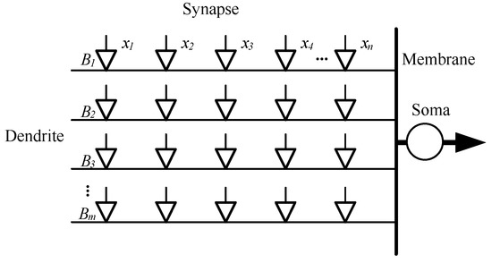
Figure 1.
Structure of LDNM.
The function of the synaptic layer is to receive input signals from other neurons and to process these input signals by using the following equation:
where is the output of the i-th () synapse on the j-th () dendritic branch; k is a fixed parameter, which is set to 5; is the input to the synapse, which is in [0, 1]; and and are the connection parameters that we need to train.
The dendritic layer receives the output signal from the synapse and performs a multiplication operation, as expressed in Equation (2), on each branch. The dendritic layer plays an important role in the transmission and processing of neural information.
Information about all dendritic branches is collected in the membrane layer. The sum of this information is calculated by Equation (3), and the output is transmitted to the soma body.
The output signal of the membrane layer is calculated in the soma body using a modified sigmoid function, which is expressed as follows:
where O is the final output; c is a fixed parameter, which is set to 5; and is the threshold of the soma body, which is set to 0.5. If this signal is greater than the threshold of the soma body, the neuron is fired.
2.1. Connection States
The connection parameters and of a synapse can determine the connection state of the synapse. There are four types of connection states, namely, direct connection, inverse connection, constant 1 connection, and constant 0 connection. After training, each synapse will be in one of the four connection states. These connection states are shown in Figure 2.
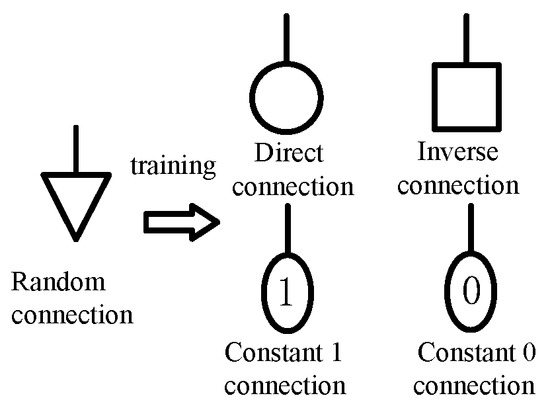
Figure 2.
Connection states of a synapse.
When , the connection state of the corresponding synapse is direct connection. When , the connection state of the synapse is inverse connection. When or , the connection state of the synapse is constant 1 connection. When or , the connection state of the synapse is constant 0 connection. In addition, a threshold is defined at each synapse, which is calculated as .
In the direct connection state, the synaptic output is approximately 1 when the input is greater than the threshold; otherwise, the output is approximately 0. In the inverse connection state, the synaptic output is approximately 0 when the input is greater than the threshold; otherwise, the output is approximately 1. In the constant 1 connection state, the synaptic output is always approximately 1, and in the constant 0 connection state, the synaptic output is always approximately 0.
2.2. Neuronal Structure Pruning
According to the connection states of the synaptic layer, LDNM can be pruned to remove unnecessary synapses and dendrites. The structure of LDNM is simplified. There are two pruning mechanisms operating on LDNM: synaptic pruning and dendritic pruning.
Synaptic pruning: When a synapse is in the constant 1 connection state, the synaptic output is always approximately 1, so the output value of the synapse has no effect on the result of a multiplication operation. Thus, any synapse in the constant 1 connection state can be omitted.
Dendritic pruning: When a synapse is in the constant 0 connection state, the synaptic output is always approximately 0. When 0 is involved in a multiplication operation, the result of the operation is always 0. In this case, the output of the dendritic branch is always 0, regardless of the values of the other synapses on the branch. When an addition operation is performed in the membrane layer, 0 can be omitted without affecting the result. Thus, any dendritic branch that contains a synapse in the constant 0 connection state can be omitted.
Figure 3 depicts examples of the synaptic pruning and dendritic pruning operations.
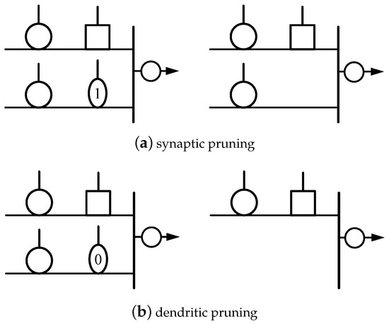
Figure 3.
Synaptic pruning and dendritic pruning can be performed on a trained LDNM.
3. Training Algorithm
The GBO algorithm is a heuristic algorithm for solving complex optimization problems that combines population and gradient approaches. It uses a set of vectors and two main operators to explore the search space. These two operators are the gradient search rule and the local escape operator.
3.1. Gradient Search Rule
The gradient search rule (GSR) uses a gradient-based method to improve the search trend, accelerate the convergence and obtain a better solution in the search space. The i-th element of can be calculated as follows:
where is a normally distributed random number, is a small number within the range of [0, 0.1], and are the best and worst solutions obtained during the optimization process, and is determined based on the difference between the best solution () and a randomly selected position ().
where and are 0.2 and 1.2, respectively; is a random number in [0, 1]; m is the current number of iterations; and M is the maximum number of iterations. The motion direction is added to make better use of the area near .
Based on and , the search is performed under the condition of focusing on global search:
or under the condition of focusing on local search:
where is a randomly selected position and . GBO uses these two search methods to enhance exploration and exploitation. Therefore, the new solution for the next iteration can be defined as follows:
where and are two random numbers in [0, 1].
3.2. Local Escape Operator
To improve the efficiency of the GBO algorithm in solving complex problems, a local escape operator (LEO) is introduced. This operator can significantly change the position of the solution to avoid local convergence. The GBO algorithm has a probability of executing LEO, which is set to 0.1. The LEO execution strategy is described in Equation (15).
where is a uniform random number in ; is a random number obeying the standard normal distribution; and , , and are defined as follows:
where and are random numbers in [0, 1], is a vector with randomly generated elements, and is a random individual in the population.
3.3. Training Process
The purpose of the LDNM training process is to optimize the combination of connection parameters and in the synaptic layer to improve the classification performance of LDNM. LEO enables the GBO algorithm to jump out of local optima. GSR accelerates the convergence of the GBO algorithm, which avoids the deficiency of the BP algorithm and further improves the classification performance of LDNM. Therefore, the GBO algorithm is more suitable for training LDNM than the BP algorithm.
We encode these connection parameters into a vector . The GBO algorithm is used to optimize this vector. The process of training LDNM with the GBO algorithm is shown in Figure 4. First, the GBO algorithm randomly initializes the individuals in the population. The population size N is set to 50, and each individual is represented by a vector , which corresponds to the n-th individual in the population of the m-th generation of the iteration. Each individual inputs its own saved w and q into LDNM and calculates its respective fitness based on the value output by LDNM. After calculating the fitness values of all individuals, the best and worst individuals, and , are identified, and then the GSR operator is executed on all individuals to generate the next generation of individuals. After performing the GSR operator on an individual, there is a probability that the LEO operator will be executed to prevent the algorithm from falling into a local optimum. GBO iterates the process until the maximum number of iterations M is reached. Finally, is returned as the optimization result, which contains the optimized LDNM connection parameters.
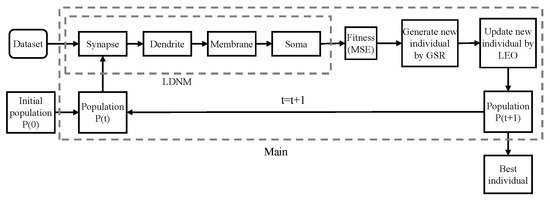
Figure 4.
Flowchart of LDNM training using the GBO algorithm.
The GBO algorithm uses the mean square error (MSE) as the fitness function. It can be calculated as follows:
where J is the number of training set samples, is the model output value of the j-th sample, and is the actual label value of the j-th sample.
4. Experimental Study
The experiments in this study are implemented in the Java and Python languages. All experiments are run on a Windows 10 system that has a 1.6 GHz i5 CPU and 8 GB RAM.
4.1. Dataset Description
Seven datasets are used in the experiments to evaluate the performance of LDNM: Iris, Seed, Wine, Parkinson, Migraine, Forest type mapping (FTM), and Breast Cancer(BC). These seven datasets can be accessed from the UCI Machine Learning Repository and Kaggle. Table 1 reports information about these seven datasets. Notably, this study focuses on binary classification problems. We preprocess multiclass classification datasets into binary classification datasets by labeling one of the classes as the positive class and the rest as the negative class.

Table 1.
Information on the seven datasets.
The Iris dataset is a classic dataset that contains 3 types of irises and 4 features. The Seed dataset consists of seeds of three types of wheat varieties. Each type has 70 data and seven feature values. These feature values can be used to determine the variety of wheat. The Wine dataset includes chemical composition analysis results for wines from specific Italian regions. The origin of each wine can be inferred from the chemical composition. The Parkinson dataset [33] consists of biomedical speech measurements from 31 individuals, 23 of whom have Parkinson’s disease. Voice recordings are used to distinguish between healthy people and Parkinson’s patients. The Migraine dataset contains 400 samples, each with 23 features. The FTM dataset [34] contains multitemporal remote sensing data of a forest area in Japan, and the goal is to map different forest types using spectral data. The BC dataset has 569 samples, each with 30 features. These feature values can be used to determine whether the tumor is malignant or benign.
Each dataset in the experiment is randomly divided into a training set and test set, with each accounting for 50% of all samples in the dataset. For each dataset, the experiment is independently executed 30 times. Each machine learning method is trained on the training set and evaluated on the test set. To fit the input of LDNM, the feature values of the datasets are normalized to [0, 1].
4.2. Experimental Configuration
To train LDNM with the GBO algorithm, the connection parameters (w and q) in each neuron are encoded into the solution vector of the GBO algorithm, and then LDNM is trained according to the procedure described above. w and q are initialized randomly within in the experiments [18]. The length of the vectors in GBO is calculated as follows:
where I is the number of inputs (number of features in the dataset) and B is the number of dendritic branches. B is usually set to the value of I.
The performance of the algorithm is evaluated using the classification accuracy on the test set, and the accuracy is defined as follows:
where E denotes the number of correctly predicted samples in the test set and A denotes the total number of samples in the test set.
4.3. Comparison with the BP Algorithm
The BP algorithm is the original training algorithm of LDNM, which updates the training parameters by using error backpropagation. However, the BP algorithm has various disadvantages, such as slow convergence and ease of falling into local convergence when training LDNM. In this section, we compare the GBO algorithm and BP algorithm in terms of LDNM training performance. To fairly compare the performances of the two algorithms, 20,000 iterations are performed by the BP algorithm and 400 iterations by the GBO algorithm in training LDNM. In this configuration, BP requires more training time and memory than GBO. The BP algorithm for training LDNM uses the implementation in [35]. The comparison results are reported in Table 2. The results show that the MSE of the GBO algorithm is smaller than that of the BP algorithm on all seven datasets. This indicates that the GBO algorithm has an advantage over the BP algorithm in terms of convergence. The classification accuracy of the LDNM trained by the GBO algorithm is higher than that of the LDNM trained by the BP algorithm on all seven datasets. In particular, the classification accuracy of the BP algorithm is more than 10% lower than that of the GBO algorithm on the Wine, Parkinson, Migraine, FTM, and BC datasets. To test whether there is a significant difference between the training results of the two algorithms, we perform the Wilcoxon signed rank test. The significance level is set to 0.05. Table 2 shows that the p values are smaller than 0.05 on the six datasets, indicating that the training results of the GBO algorithm are significantly better than those of the BP algorithm on the six datasets. However, there is no significant difference between the two algorithms on the Iris dataset.
Table 2.
Comparison results of the GBO algorithm and BP algorithm on the seven datasets.
Figure 5 shows the convergence curves of the GBO algorithm and the BP algorithm for training LDNM on the seven datasets. On both the Iris and Seed datasets, the number of features is below 10. The BP algorithm can train LDNM well, and there is no obvious gap in the convergence trend between the BP and GBO algorithms. On the Wine dataset, the number of features reaches 13. The MSE of the BP algorithm is approximately 0.04, and the MSE of the GBO algorithm is below 0.01. The GBO algorithm converges better than the BP algorithm. On the other datasets, the number of features exceeds 20. At this point, the BP algorithm almost does not converge, indicating that the BP algorithm is trapped in a local optimum. In contrast, the unique LEO operator of the GBO algorithm enables it to avoid this problem. The experimental results show that the convergence of the BP algorithm deteriorates as the number of features of the dataset increases, while the GBO algorithm is not significantly affected.
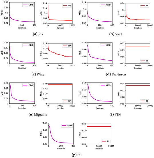
Figure 5.
Convergence curves of the GBO algorithm and BP algorithm on the seven datasets.
4.4. Comparison with Other Heuristic Algorithms
In this section, we compare the GBO algorithm with four other heuristic algorithms in training LDNM. Among them, PSO, DE, and GA are classic heuristic algorithms. The EO algorithm is a relatively new algorithm with a novel design and is highly competitive. To ensure the fairness of the comparison experiments, the key parameters of each algorithm are set to the values suggested in the literature [28,30,31,32]. In addition, these algorithms use the same fitness function as GBO and are iterated 400 times when training LDNM.
The classification results are summarized in Table 3. The accuracy of LDNM after training by the GBO algorithm is the highest on the six datasets. On the Migraine dataset, the best performer is the DE algorithm, with GBO ranking second. To further determine whether there are significant differences among the training results of the GBO algorithm and the other heuristic algorithms, we perform the Friedman test on the classification results. The Friedman test can be used to determine whether there are significant differences among multiple sets of data. The algorithm with the smallest rank value has the best performance. The Friedman test results are shown in Table 4. The GBO algorithm has the smallest rank value, indicating that the LDNM trained by the GBO algorithm achieves the best performance. To avoid Type I error [36], we use the Bonferroni correction to adjust the p values (). The results show that the values of the GA and PSO are less than the significance level of 0.05. Therefore, there is a significant difference between the GBO algorithm and the two algorithms in training LDNM. Moreover, there are no significant differences between the GBO algorithm and the remaining algorithms. Overall, compared with these four heuristic algorithms, the GBO algorithm performs better or very competitively in training LDNM.
Table 3.
Classification results of the five heuristic algorithms on the seven datasets.
Table 4.
Friedman test of the comparison results reported in Table 3.
Figure 6 shows the convergence curves of the five heuristic algorithms for training LDNM on each dataset. On the Iris dataset, the GBO algorithm converges the best, and the other four algorithms converge very close to but slightly worse than the GBO algorithm. On the Seed dataset, the GBO, PSO and EO algorithms converge very close to each other, and the DE and GA algorithms perform poorly. On the Wine dataset, the GBO algorithm converges the best. In addition, the GBO algorithm converges significantly better than the other four algorithms on the Parkinson dataset. The number of features exceeds 20 for the dataset. The GBO algorithm converges best on the remaining dataset. However, it did not pull away from DE, PSO, and EO algorithms. In addition, the convergence of the GA algorithm is significantly inferior to the other algorithms. These results show that the GBO algorithm can serve as a competitive training method in solving complex problems.
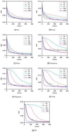
Figure 6.
Convergence curves of five heuristic algorithms for training LDNM.
4.5. Comparison with Other Classifiers
The above experiments demonstrate that the GBO algorithm is a perfect algorithm for training LDNM. Next, we verify the classification performance of LDNM/GBO, and we compare it with five classic classifiers. These five classifiers are linear support vector machine (linear SVM), naive Bayes (NB), decision tree (DT), random forest (RF), and multilayer perceptron (MLP).
In the experiments, the classifiers are implemented using the scikit-learn machine learning library [37], and their parameters are set to the recommended values in scikit-learn. Table 5 shows the classification results of all classifiers. Among them, LDNM/GBO has the highest classification accuracy on four datasets, namely, Iris, Seed, Wine and Parkinson. On the FTM dataset, the best performer is MLP, and LDNM/GBO does not have a high accuracy and ranks only fifth. LDNM/GBO ranked second and third on the Migraine and BC datasets, respectively. Overall, LDNM/GBO has excellent classification performance. We use the Friedman test to examine the accuracy of these classifiers and report the statistical results in Table 6. The results show that the rank value of LDNM/GBO is the smallest, so the classification performance of this classifier is considered the best. Finally, the p values are adjusted using Bonferroni correction. The adjusted p value of NB is below the significance level of 0.05. This indicates that there is a significant difference between LDNM/GBO and NB. However, there is no significant difference between LDNM/GBO and the other four classifiers. The experimental results indicate that LDNM/GBO is a highly competitive classifier.
Table 5.
Classification results of LDNM/GBO and other classifiers.
Table 6.
Friedman test of the comparison results reported in Table 5.
4.6. Pruning Results
The trained LDNM can be simplified by synaptic pruning and dendritic pruning. Figure 7 shows the typical structures of the pruned LDNM for each dataset. We find that the number of features of the pruned LDNM is smaller than that of the trained LDNM. This indicates that synaptic pruning can remove unnecessary features and preserve useful features. In addition, compared with the trained LDNM, the pruned LDNMs have greatly reduced numbers of dendritic branches. Only two dendritic branches remain in the corresponding LDNM on three datasets. On the Migraine, FTM, and BC datasets, the pruned LDNM ends up with only one dendritic branch. This finding indicates that the dendritic pruning of LDNM effectively removes the useless dendritic branches.
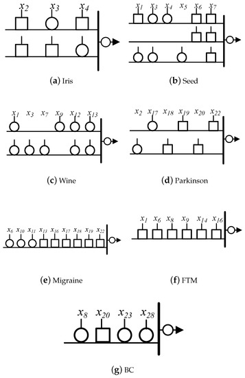
Figure 7.
Typical structures of the pruned LDNM for each dataset.
Table 7 reports the classification results of the LDNM trained by the GBO algorithm and the pruned LDNM on seven datasets. On the Iris and Wine datasets, the accuracy of the pruned LDNM is lower than that of the trained LDNM, but the difference is less than 0.5%. On the Seed dataset, the accuracy of the pruned LDNM is improved. On the Parkinson and FTM datasets, the difference in classification accuracy of LDNM before and after pruning is around 1%. On the Migraine and BC datasets, the classification accuracy difference between LDNM before and after pruning is around 2%. These results indicate that there is no significant difference between the trained LDNM and the pruned LDNM. The structure pruning operation does not lead to a dramatic reduction in the classification accuracy of the trained LDNM.
Table 7.
Classification results of the trained LDNM and pruned LDNM for each dataset.
5. Conclusions
In this paper, we used the GBO algorithm to train a logic dendritic neuron model to solve classification problems. GBO is a heuristic algorithm that is effective in avoiding falling into local optima and enables LDNM to solve high-dimensional problems. In our experiments, we used seven datasets to verify the effectiveness of the GBO algorithm. First, the GBO algorithm was compared with the BP algorithm, which is a common training algorithm of LDNM. The results showed that compared with LDNM trained by BP, LDNM trained by the GBO algorithm showed greatly improved performance. Then, we compared the GBO algorithm with four heuristic algorithms, and the results verified the superiority of the GBO algorithm. In addition, we compared LDNM/GBO with five classic machine learning methods, and the experimental results proved that LDNM/GBO is a very competitive classifier. Finally, we pruned the trained LDNM to investigate whether the proposed neuronal structure pruning mechanisms are effective. The fine classification results and the simplified structures of the pruned LDNMs proved the reliability of the neuronal structure pruning mechanisms.
In the future, we plan to apply LDNM to solve other problems to verify its effectiveness. In addition, the classification result of LDNM requires further explanation.
Author Contributions
Conceptualization, S.S. and Q.X.; methodology, S.S. and Q.X.; software, Q.X.; validation, J.Q., Z.S. and X.C.; formal analysis, Q.X.; investigation, S.S. and J.Q.; resources, S.S. and J.Q.; data curation, S.S. and Q.X.; writing—original draft preparation, S.S. and Q.X.; writing—review and editing, J.Q., Z.S. and X.C.; visualization, S.S. and Q.X.; supervision, S.S. and J.Q.; project administration, S.S.; and funding acquisition, S.S. and X.C. All authors have read and agreed to the published version of the manuscript.
Funding
This work was supported by the Natural Science Foundation of Jiangsu Province of China (Grant No. BK20220619), the National Natural Science Foundation of China (Grant No. 62203069), and the Japan Science and Technology Agency SPRING (Grant No. JPMJSP2145).
Informed Consent Statement
Informed consent was obtained from all subjects involved in the study.
Data Availability Statement
All data are contained within the article.
Conflicts of Interest
The authors declare no conflict of interest.
References
- London, M.; Häusser, M. Dendritic computation. Annu. Rev. Neurosci. 2005, 28, 503–532. [Google Scholar] [CrossRef] [PubMed]
- Agmon-Snir, H.; Carr, C.E.; Rinzel, J. The role of dendrites in auditory coincidence detection. Nature 1998, 393, 268–272. [Google Scholar] [CrossRef] [PubMed]
- Koch, C.; Poggio, T.; Torre, V. Nonlinear interactions in a dendritic tree: Localization, timing, and role in information processing. Proc. Natl. Acad. Sci. USA 1983, 80, 2799–2802. [Google Scholar] [CrossRef] [PubMed]
- Koch, C.; Poggio, T.; Torre, V. Retinal ganglion cells: A functional interpretation of dendritic morphology. Philos. Trans. R. Soc. Lond. B Biol. Sci. 1982, 298, 227–263. [Google Scholar]
- Destexhe, A.; Marder, E. Plasticity in single neuron and circuit computations. Nature 2004, 431, 789–795. [Google Scholar] [CrossRef]
- Legenstein, R.; Maass, W. Branch-specific plasticity enables self-organization of nonlinear computation in single neurons. J. Neurosci. 2011, 31, 10787–10802. [Google Scholar] [CrossRef]
- Ji, J.; Gao, S.; Cheng, J.; Tang, Z.; Todo, Y. An approximate logic neuron model with a dendritic structure. Neurocomputing 2016, 173, 1775–1783. [Google Scholar] [CrossRef]
- Ji, J.; Song, S.; Tang, Y.; Gao, S.; Tang, Z.; Todo, Y. Approximate logic neuron model trained by states of matter search algorithm. Knowl.-Based Syst. 2019, 163, 120–130. [Google Scholar] [CrossRef]
- Tang, C.; Ji, J.; Tang, Y.; Gao, S.; Tang, Z.; Todo, Y. A novel machine learning technique for computer-aided diagnosis. Eng. Appl. Artif. Intell. 2020, 92, 103627. [Google Scholar] [CrossRef]
- Zhou, T.; Gao, S.; Wang, J.; Chu, C.; Todo, Y.; Tang, Z. Financial time series prediction using a dendritic neuron model. Knowl.-Based Syst. 2016, 105, 214–224. [Google Scholar] [CrossRef]
- Song, Z.; Tang, Y.; Ji, J.; Todo, Y. Evaluating a dendritic neuron model for wind speed forecasting. Knowl.-Based Syst. 2020, 201–202, 106052. [Google Scholar] [CrossRef]
- Luo, X.; Wen, X.; Zhou, M.; Abusorrah, A.; Huang, L. Decision-Tree-Initialized Dendritic Neuron Model for Fast and Accurate Data Classification. IEEE Trans. Neural Netw. Learn. Syst. 2022, 33, 4173–4183. [Google Scholar] [CrossRef] [PubMed]
- Hagan, M.T.; Menhaj, M.B. Training feedforward networks with the Marquardt algorithm. IEEE Trans. Neural Netw. 1994, 5, 989–993. [Google Scholar] [CrossRef] [PubMed]
- Zhang, N. An online gradient method with momentum for two-layer feedforward neural networks. Appl. Math. Comput. 2009, 212, 488–498. [Google Scholar] [CrossRef]
- Song, Z.; Tang, C.; Ji, J.; Todo, Y.; Tang, Z. A Simple Dendritic Neural Network Model-Based Approach for Daily PM2.5 Concentration Prediction. Electronics 2021, 10, 373. [Google Scholar] [CrossRef]
- Bianchini, M.; Gori, M. Optimal learning in artificial neural networks: A review of theoretical results. Neurocomputing 1996, 13, 313–346. [Google Scholar] [CrossRef]
- Vogl, T.P.; Mangis, J.K.; Rigler, A.K.; Zink, W.T.; Alkon, D.L. Accelerating the convergence of the back-propagation method. Biol. Cybern. 1988, 59, 257–263. [Google Scholar] [CrossRef]
- Song, S.; Chen, X.; Tang, C.; Song, S.; Tang, Z.; Todo, Y. Training an approximate logic dendritic neuron model using social learning particle swarm optimization algorithm. IEEE Access 2019, 7, 141947–141959. [Google Scholar] [CrossRef]
- Del Ser, J.; Osaba, E.; Molina, D.; Yang, X.S.; Salcedo-Sanz, S.; Camacho, D.; Das, S.; Suganthan, P.N.; Coello, C.A.C.; Herrera, F. Bio-inspired computation: Where we stand and what’s next. Swarm Evol. Comput. 2019, 48, 220–250. [Google Scholar] [CrossRef]
- Chen, X.; Song, S.; Ji, J.; Tang, Z.; Todo, Y. Incorporating a multiobjective knowledge-based energy function into differential evolution for protein structure prediction. Inf. Sci. 2020, 540, 69–88. [Google Scholar] [CrossRef]
- Song, S.; Chen, X.; Zhang, Y.; Tang, Z.; Todo, Y. Protein–ligand docking using differential evolution with an adaptive mechanism. Knowl.-Based Syst. 2021, 231, 107433. [Google Scholar] [CrossRef]
- Cheng, J.; Xu, P.; Xiong, Y. An improved artificial electric field algorithm and its application in neural network optimization. Comput. Electr. Eng. 2022, 101, 108111. [Google Scholar] [CrossRef]
- Soni, N.; Sharma, E.K.; Kapoor, A. Hybrid meta-heuristic algorithm based deep neural network for face recognition. J. Comput. Sci. 2021, 51, 101352. [Google Scholar] [CrossRef]
- Mathe, M.; Padmaja, M.; Tirumala Krishna, B. Intelligent approach for artifacts removal from EEG signal using heuristic-based convolutional neural network. Biomed. Signal Process. Control 2021, 70, 102935. [Google Scholar] [CrossRef]
- Stanley, K.O.; Clune, J.; Lehman, J.; Miikkulainen, R. Designing neural networks through neuroevolution. Nat. Mach. Intell. 2019, 1, 24–35. [Google Scholar] [CrossRef]
- Tang, C.; Todo, Y.; Ji, J.; Lin, Q.; Tang, Z. Artificial immune system training algorithm for a dendritic neuron model. Knowl.-Based Syst. 2021, 233, 107509. [Google Scholar] [CrossRef]
- Ahmadianfar, I.; Bozorg-Haddad, O.; Chu, X. Gradient-based optimizer: A new metaheuristic optimization algorithm. Inf. Sci. 2020, 540, 131–159. [Google Scholar] [CrossRef]
- Bonyadi, M.R.; Michalewicz, Z. Particle swarm optimization for single objective continuous space problems: A review. Evol. Comput. 2017, 25, 1–54. [Google Scholar] [CrossRef]
- Song, S.; Ji, J.; Chen, X.; Gao, S.; Tang, Z.; Todo, Y. Adoption of an improved PSO to explore a compound multi-objective energy function in protein structure prediction. Appl. Soft Comput. 2018, 72, 539–551. [Google Scholar] [CrossRef]
- Pant, M.; Zaheer, H.; Garcia-Hernandez, L.; Abraham, A. Differential Evolution: A review of more than two decades of research. Eng. Appl. Artif. Intell. 2020, 90, 103479. [Google Scholar]
- Mirjalili, S.; Song Dong, J.; Sadiq, A.S.; Faris, H. Genetic algorithm: Theory, literature review, and application in image reconstruction. Nat.-Inspired Optim. 2020, 69–85. [Google Scholar]
- Faramarzi, A.; Heidarinejad, M.; Stephens, B.; Mirjalili, S. Equilibrium optimizer: A novel optimization algorithm. Knowl.-Based Syst. 2020, 191, 105190. [Google Scholar] [CrossRef]
- Little, M.; Mcsharry, P.; Roberts, S.; Costello, D.; Moroz, I. Exploiting nonlinear recurrence and fractal scaling properties for voice disorder detection. Nat. Preced. 2007, 1. [Google Scholar]
- Johnson, B.; Tateishi, R.; Xie, Z. Using geographically weighted variables for image classification. Remote Sens. Lett. 2012, 3, 491–499. [Google Scholar] [CrossRef]
- Song, S.; Chen, X.; Song, S.; Todo, Y. A neuron model with dendrite morphology for classification. Electronics 2021, 10, 1062. [Google Scholar] [CrossRef]
- Garcıa, S.; Molina, D.; Lozano, M.; Herrera, F. A study on the use of non-parametric tests for analyzing the evolutionary algorithms’ behaviour: A case study on the CEC’2005 special session on real parameter optimization. J. Heuristics 2009, 15, 617–644. [Google Scholar] [CrossRef]
- Pedregosa, F.; Varoquaux, G.; Gramfort, A.; Michel, V.; Thirion, B.; Grisel, O.; Blondel, M.; Prettenhofer, P.; Weiss, R.; Dubourg, V.; et al. Scikit-learn: Machine learning in Python. J. Mach. Learn. Res. 2011, 12, 2825–2830. [Google Scholar]
Disclaimer/Publisher’s Note: The statements, opinions and data contained in all publications are solely those of the individual author(s) and contributor(s) and not of MDPI and/or the editor(s). MDPI and/or the editor(s) disclaim responsibility for any injury to people or property resulting from any ideas, methods, instructions or products referred to in the content. |
© 2022 by the authors. Licensee MDPI, Basel, Switzerland. This article is an open access article distributed under the terms and conditions of the Creative Commons Attribution (CC BY) license (https://creativecommons.org/licenses/by/4.0/).