1. Introduction
Retinal fundus pictures are commonly used to diagnose many eye-related illnesses that lead to blindness, such as macular degeneration and diabetic retinopathy [
1]. A direct ophthalmoscope, or the manual inspection of the fundus by a professional, is being replaced by a computer-assisted diagnosis of retinal fundus images. Furthermore, the computer-assisted diagnosis of retinal fundus images is as accurate as a direct ophthalmoscope and requires less processing and analysis time. The extraction of retinal blood vessels from fundus pictures is one of the essential processes in detecting diabetic retinopathy. Even though numerous segmentation approaches have been proposed, segmentation of the retinal vascular network and picture quality remains difficult. Noise (typically owing to uneven lighting) and narrow vessels are now the critical obstacles in retinal vascular segmentation.
Although most vessel segmentation methods include pretreatment procedures to improve vessel appearance, other plans skip the pre-processing steps and jump straight to the segmentation stage [
2]. Additionally, most of the proposed segmentation algorithms optimise the pre-processing and vessel segmentation parameters for each dataset separately. As a result, these algorithms can typically achieve high accuracy for the optimised dataset, but their accuracy will be lowered when applied to different datasets.
Many segmentation approaches nowadays use machine learning ideas in conjunction with traditional techniques to improve the segmentation accuracy by providing a statistical analysis of the data to enhance segmentation algorithms [
3]. Based on the usage of labelled training data, these machine learning principles can be divided into unsupervised and supervised approaches. A supervised technique, a human operator labels and assigns a class to each pixel in the image, such as vessel and non-vessel. A classifier is trained using the tags supplied to the input. A sequence of feature vectors is formed from the data being processed (pixel-wise features in image segmentation problems). In an unsupervised technique, similar samples are grouped into various classes using predetermined feature vectors without any class labels. This clustering is based on several assumptions about the input data structure, namely, that there are two classes of input data with identical feature vectors (vessel and not vessel). Depending on the situation, this similarity metric might be sophisticated or specified by a simple metric, such as pixel intensities [
4].
The detection of the vascular tree in fundus images with precision and accuracy can provide several essential aspects for diagnosing various retinal disorders. However, when utilised as a pre-processing step for higher-level picture analysis, retinal blood vessel segmentation might significantly impact other applications. For instance, reliable blood vessel tree detection can be employed in registering time series fundus images, finding the optic disc or over, recognising the retinal nerve fibre layer, and biometric identification. There is substantial work on this topic due to the wide range of applications and the fact that segmentation of retinal vessels is one of the most challenging jobs in retinal image processing [
5].
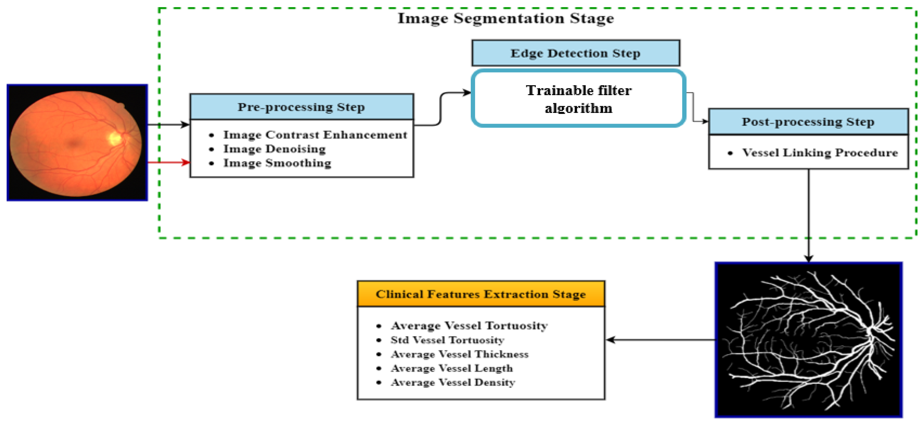
An accurate, rapid, and fully automatic blood vessel segmentation and clinical features measurement algorithm for retinal fundus images is proposed to improve the diagnosis precision and decrease the workload of the ophthalmologists. The main pipeline of the proposed algorithm is composed of two essential stages: image segmentation and clinical features extraction stage. In the segmentation stage, a fully automated segmentation algorithm is proposed and named a trainable filtering algorithm to detect the blood vessels in the retinal images accurately. An efficient and reliable image pre-processing procedure in the trainable filtering algorithm is applied to increase the contrast level. To improve or enhance the intensity level of the small objects in the retinal blood vessel structure, contrast limited adaptive histogram equalisation (CLAHE) and improved complex wavelet transform (I-CWT), respectively, are used by removing all the undesired objects (e.g., small vessel segments) in the enhanced image by applying the Vessels Detection Stage. Finally, the retinal blood vessels are detected using an efficient edge detection algorithm based on an improved Canny edge detector. Finally, the output segmented images produced from the proposed algorithm are fused to produce the final segmented image. In the post-processing step, a novel blood vessel linking procedure is proposed to correctly join the discontinuous blood vessels produced in the segmented image resulting from the previous step. Several useful clinical features are computed, such as the blood vessel’s tortuosity, length, density, and thickness, which are efficiently used in the early diagnosis of several cardiovascular and ophthalmologic diseases. An efficient and accurate algorithm for computing the blood vessel thickness is proposed in this stage. The main contributions list can be summarised as follows:
An accurate, rapid, and fully automatic blood vessel segmentation and clinical features measurement algorithm for retinal fundus images is proposed to improve the diagnosis precision and decrease the workload of the ophthalmologists.
The fully automated segmentation algorithm is proposed and named a trainable filtering algorithm to accurately detect the delicate blood vessels in the retinal images.
A novel blood vessel linking procedure is proposed to correctly join the discontinuous blood vessels produced in the segmented image resulting from the previous step.
The rest of this study is organised as follows:
Section 2 presents related works on a fully automatic blood vessel segmentation and clinical features measurement algorithm for retinal fundus images. The main steps of the proposed trainable filtering algorithm, composed of two main stages, including the image pre-processing stage and the vessels detection stage, are presented in
Section 3.
Section 4 provides several extensive experiments to evaluate the performance and accuracy of the developed hybrid and fully automated segmentation algorithm for detecting the retinal blood vessels using two extremely challenging fundus images datasets. Finally, the conclusion and future work are discussed in
Section 5.
2. Related Works
Automated techniques for medical image analysis have become essential due to the large volume of patient information that needs to be processed. Manual analysis can be reduced or avoided by achieving high accuracy from the retinal blood vessels tree auto segmentation. According to Maitreya et al. [
6], they used trainable semantic segmentation by utilizing a hybrid method to solve the resolution issue by implementing an artificial neural network and Capsule Network to achieve up to 99.01% and 98.7%, respectively. The approach proposed by [
7] works on breast cancer boundary and pectoral muscle in mammogram images through implementing several algorithms, such as the improved threshold-based and trainable via use mammographic image analysis society and breast cancer digital repository. The proposed study achieved 98.6% accuracy even though the authors highlight that mammogram segmentation is still an open research problem and has to be improved. Reference [
8] utilized the fully-convolutional networks U-Nets to improve the segmentation and detection in the medical images by using two different datasets, which are ECU and HGR, and their average output results were 92.3% and 94%, respectively. The researcher focused on enhancing the idea of the contextual pixel analysis through utilizing the lower numbers of trainable parameters and thus gives the space open to future work to increase the numbers. According to [
9], they are working on a conventional neural network method for the segmentation of retinal images via the used dataset of 50 colour images that produced 0.95 average accuracies. Failing to observe the progress of some dangerous disease leads to the development of a particular abnormality in the retinal vessels that might damage the retina. Soaibuzzaman et al. [
10] worked on an image segmentation based on convolutional neural networks and trainable methods. The most common datasets—PASCAL VOC 2012 and Citypass—are used to perform the proposed algorithms.
Ali Hatamizadeh et al. [
11] presented trainable deep active contours (TDACs) to implement in the image segmentation framework to solve the accuracy issue using the vaihingen and bing huts datasets. In addition, a modern hybrid method was proposed; but, we noticed some points that could limit the applicability, such as dependence on pre-trained convolutional neural networks. Moreover, they leave the area open for further enhancement on the accuracy of CNN-based image segmentation. They might stop at one point and open the space to future work enhancement. Eventually, the studies present in this section mostly all focused on enhancing the accuracy of the segmented retinal images. Therefore, this paper highlights the trainable filter algorithm adapted with very powerful and common datasets, DRIVE and HRF, to achieve the highest accuracy results of up to 99.12% and 98.78%, respectively.
3. The Proposed Automatic Blood Vessels Segmentation and Clinical Features Measurement Algorithm
A fully automated algorithm is presented for detecting the retinal blood vessels in the highly challenging fundus images. A quantitative investigation of retinal images is widely used to diagnose, screen, and treat disease. Among these diseases mentioned, diabetic retinopathy and macular degeneration are the two main reasons for vision loss. Blood vessel segmentation is an essential step required for the quantitative investigation of retinal images. A set of critically beneficial clinical features, such as the blood vessel’s tortuosity, length, density, and thickness, can be extracted from the segmented vascular tree.
Furthermore, the segmented vascular tree has also been used in several medical applications, including the retinal image mosaic structure, temporary or multi-modal image registration, optic disc identification, biometric identification, and fovea localization. Accordingly, an automatic algorithm for segmenting and extracting useful clinical features from the retinal blood vessels is proposed to help ophthalmologists and eye specialists diagnose different retinal diseases and treatment assessments early.
Figure 1 shows the projected blood vessel segmentation and clinical features measurement algorithm.
3.1. The Trainable Filtering Algorithm
As presented in
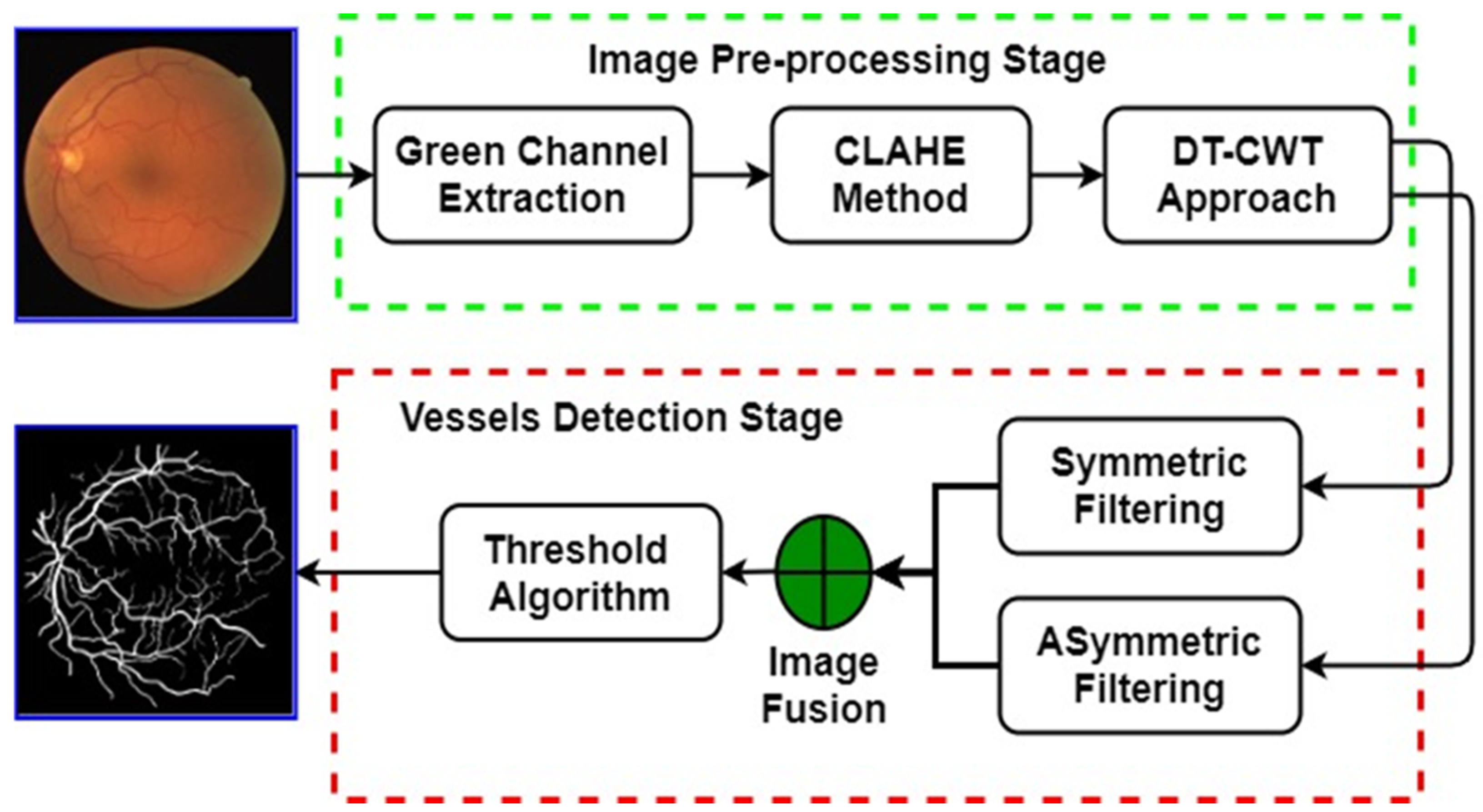
Figure 2, the proposed trainable filters algorithm consists of two main stages: image pre-processing and vessels detection stage. In the image pre-processing stage, an efficient and reliable image enhancement procedure was proposed for reducing the noise and enhancing the quality of the retinal fundus image to make the blood vessel structures more visible. In the vessel detection stage, the fusing of the responses of two trainable and rotation-invariant filters, namely, symmetric and asymmetric filters, is firstly obtained. Then, the final segmented image is produced by applying a thresholding algorithm to the fused image. The main stages of the proposed trainable filtering algorithm are explained in detail in the next sub-sections.
3.1.1. Image Pre-Processing Stage
The main steps of the proposed image enhancement procedure in the proposed trainable filters algorithm can be summarized as follows:
The contrast of the resulting image was enhanced using the CLAHE method.
An efficient image denoising procedure was proposed based on an improved Dual-Tree Complex Wavelet Transforms (DT-CWT) approach to decompose the input image and shrinkage process to eliminate the noise in the input image.
We are applying the moving average filter to enhance the edges of the blood vessels in the retinal fundus image.
The adaptive histogram equalization (AHE) is frequently employed for image contrast enhancement by expanding the dynamic range of the image intensity so that its histogram distribution has the wanted shape [
12]. The AHE is different from the conventional histogram equalization, where the adaptive histogram is computed from a specific region in the input image. Then they are used to redistribute the brightness of the image. Thus, it can efficiently improve the local contrast for each part of an image [
13]. However, the AHE method has a bias to expand the noise in approximately homogeneous areas of an image. A variant of AHE, named contrast limited adaptive histogram equalization (CLAHE), was developed to overcome this issue by limiting the amplification [
14]. The CLAHE is a block-based processing method that improves the local contrast in small regions, called tiles instead of the entire image. Then, the adjoining tiles are fused using bilinear interpolation to reduce the artificially produced boundaries. The local contrast enhancement in the homogeneous areas can be restricted to avoid the over-enhancement of noise and lessens the edge-shadowing effects in the enhanced image.
CLAHE controls the quality of the enhanced image by two essential parameters: the Clip Limit (CL) and Block Size (BS). A high value based on the CL parameter leads to an increase in the brightness of the input image due to the low-intensity level of the input image. On the other hand, a higher value of the BS parameter expands the image intensity’s dynamic range and increases its contrast level. A novel method was proposed by Min et al. [
15] to determine the optimal value of these two parameters. The pseudo-code of the CLAHE method is shown in Algorithm 1. The contrast of the blood vessels was considered as one of the primary characteristics of the coloured retinal image. Image contrast combines the range of pixels’ intensity values and the difference between the highest and smallest pixel values. The primary purpose of the proposed image enhancement procedure using the CLAHE method is to produce a uniform intensity distribution. The image with poor contrast has a small intensity range. Thus, the CLAHE method spreads and adjusts the intensity distribution of the image to improve its contrast.
First, the coloured retinal image was split into three channels (e.g., red, green, and blue). The entire coloured retinal image was used in this stage rather than the green channel as in the proposed trainable filtering algorithm. Second, the CLAHE method was applied only to the green channel because it encodes the essential information about the blood vessel structures compared with other channels.
Finally, an improved DT-CWT was employed as a powerful image denoising approach to decrease the noise level and prevent damaging the fine details of the blood vessels (e.g., edges and curves) in the retinal image, as displayed in
Figure 3c. Typically, image denoising approaches using wavelet transform suffer from four weaknesses: shift variety, oscillations, aliasing, and shortness of directionality [
16]. Herein, an improved DT-CWT based on the shrinkage operation was employed to decrease the noise level and improve the delicate structures of the blood vessels in the retinal image. The wavelet-based shrinkage image denoising method mainly depends on thresholding the wavelet transforms coefficients where the coefficients of the small values encode the noisiest and excellent features of the image. In contrast, the essential features are encoded by the wavelet coefficients having large values. Let Y be a noisy image, X be a noiseless image, and n be the noise level.
| Algorithm 1: The pseudo-code of the CLAHE method |
- ➢
Step 1: Dividing an input image of size (M × N) pixels into non-overlapping tiles of size (8 × 8) pixels. - ➢
Step 2: Estimating the histogram of each tile according to the grey-scale levels present in an input image. - ➢
Step 3: The contrast limited histogram is computed for each tile by ( CL) value as where
refers to the average number of pixels, refers to the number of grey levels in the tile, and represent the numbers of pixels in the x and y dimensions of the specific tile. The ( CL) parameter can be computed as follows:
where refers to the actual ( CL), is the normalized ( CL) in the range of [ 0, 1]. If the number of pixels is larger than , then the pixels are clipped and the average value of the remain pixels to spread to each grey-scale level is defined as follows:
where
refers to the total number of clipped pixels. - ➢
Step 4: Redistributing the remain pixels as follows:
The program starts the search from the lowest to the highest of the grey-scale level using the above step value. If the number of pixels is less
than the program will spread 1-pixel to the grey-scale. If not all the pixels are distributed when the search is ended, the program will compute a new step according to Equation (4) and start a new search cycle until the other pixels are all distributed. - ➢
Step 5: The Rayleigh transform is employed to enhance the intensity values in each tile, as de-scribed in [ 17]. - ➢
Step 6: Computing a new grey-scale level distribution of pixels within a tile using a bi-linear interpolation among four different mappings to eliminate boundary artefacts.
|
Then, the significant steps of the wavelet-based shrinkage image denoising technique are summarized as follows:
Applying the wavelet transform
to the input image to estimate the wavelet coefficient matrix
, as in Equation (5):
We modify the coefficients of
by shrinking (thresholding) operation to get the estimate
matric of the wavelet coefficients of
.
Applying the inverse wavelet transform to the coefficients matric produced from step 2 to produce the denoised coefficients, as in Equation (7):
In this study, a soft threshold function
was implemented in step 2.
3.1.2. Vessel Detection Stage
In this stage, the retinal blood vessels were detected by fusing the responses of two Shifted Filter Responses (SRF), termed the symmetric and asymmetric filter for detecting the main blood vessels structures and the endings of the vessels, respectively (see
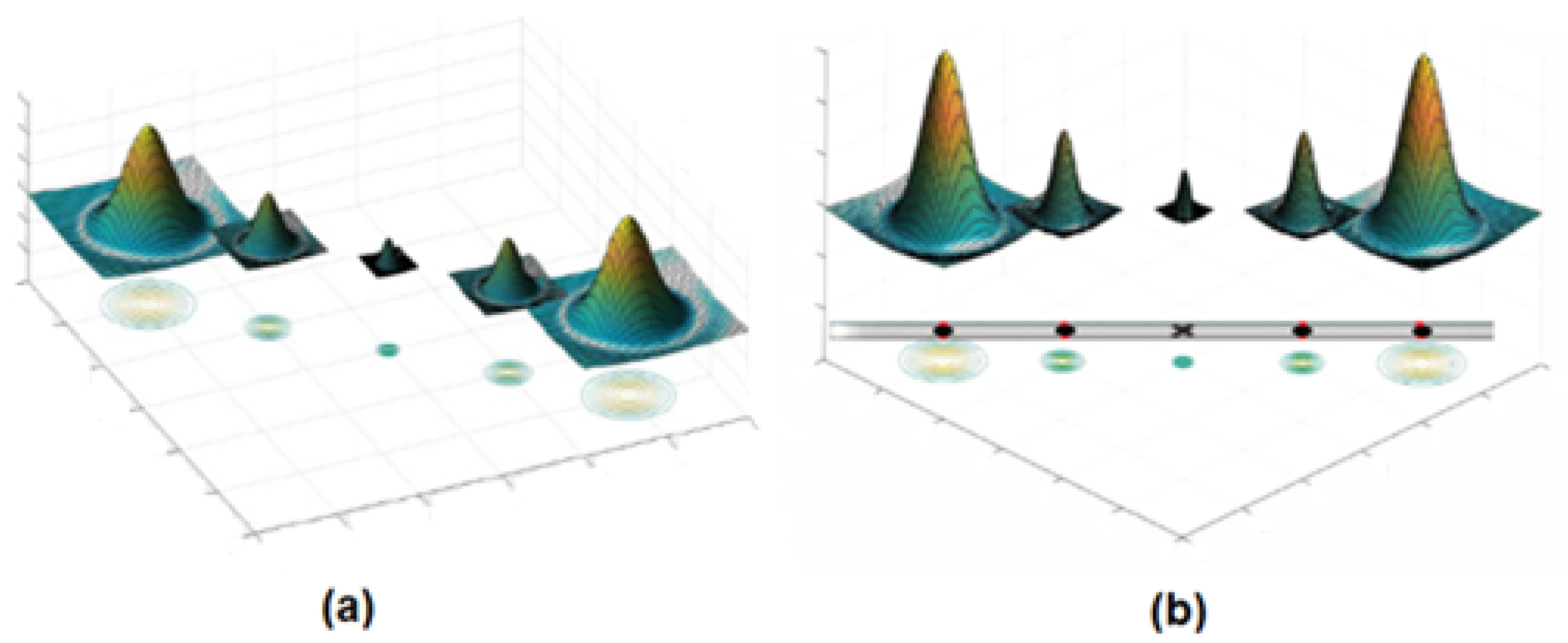
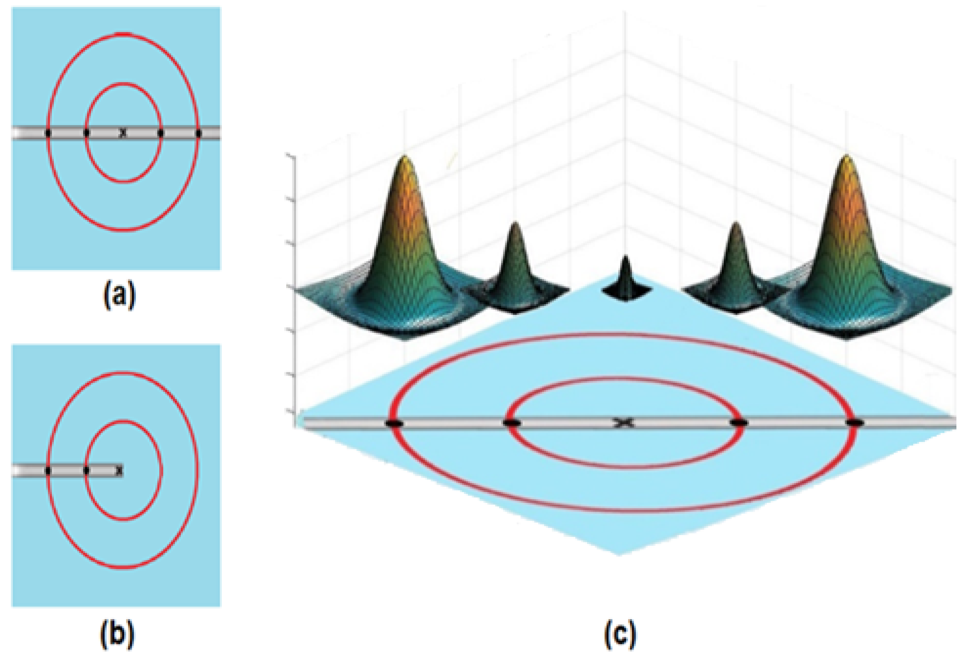
Figure 4). These two filters were rotated in 12 orientations to include all the possible directions of the retinal blood vessels. Consequently, it creates a filter bank of a 15° rotation of the filter, which is reliable and suitable for optimal retinal blood vessels detection. Then, the final segmented image was obtained by fusing the responses of these two filters and then thresholding the fused image. The proposed SRF filters are non-linear due to their ability orientation selectivity based on the output representations produced from a set of Difference of Gaussians (DoG) filters. The SRF filters are invariant to rotation, scale, translation, and reflection transformations. The selectivity of these two trainable filters is not pre-defined in the implementation process. However, it is defined from operator-specified sample patterns (e.g., vertical vessels and bifurcation points) in an automated manner.
The SRF filters are unsupervised trainable edges detectors filters that can be configured to automatically detect the symmetric and asymmetric straight-edges structures of the retinal blood vessels.
Figure 5 shows how the SRF filters performed the detection process of the patterns by using the DoG filter. The input of SRF can be represented by five blobs produced from the DoG filter and placed at a specific distance from the centre of the filter, as presented in
Figure 4a. The result of the SRF filters was calculated as the weighted geometrical mean of the shifted and the blurred responses of the DoG filter.
The main steps of applying the SRF filters can be summarized as follows:
Create the DoG filter and convolute it with the retinal image as in Equations (8) and (11):
Here, refers to the centre of the DoG filter, and refers to the SD, and it is 0.5 for the inner Gaussian filter.
Blurring the gained responses of the DoG filter by applying Equation (9).
Shifting the produced blurred DoG responses to the filter centre’s direction with a shift-vector as in Equation (10).
where
refers to the Rectifying Linear Unit (ReLU). For a given
intensity distribution of an input image
, the response
of the DoG filter is
. If the output of the convolution process is negative, then it is replaced with
0 as in Equation (11). The shifted and blurred DoG responses at the location
can be defined by Equation (12).
Generating the responses of the SRF filters by calculating the geometric mean, as in Equation (13).
where
,
,
.
As in Equation (13), the DoG responses of the SRF filters for each retinal image were thresholded by using a specific parameter (t) value to classify the image’s pixels into two classes: blood vessels or non-blood vessels.
3.2. Post-Processing Step
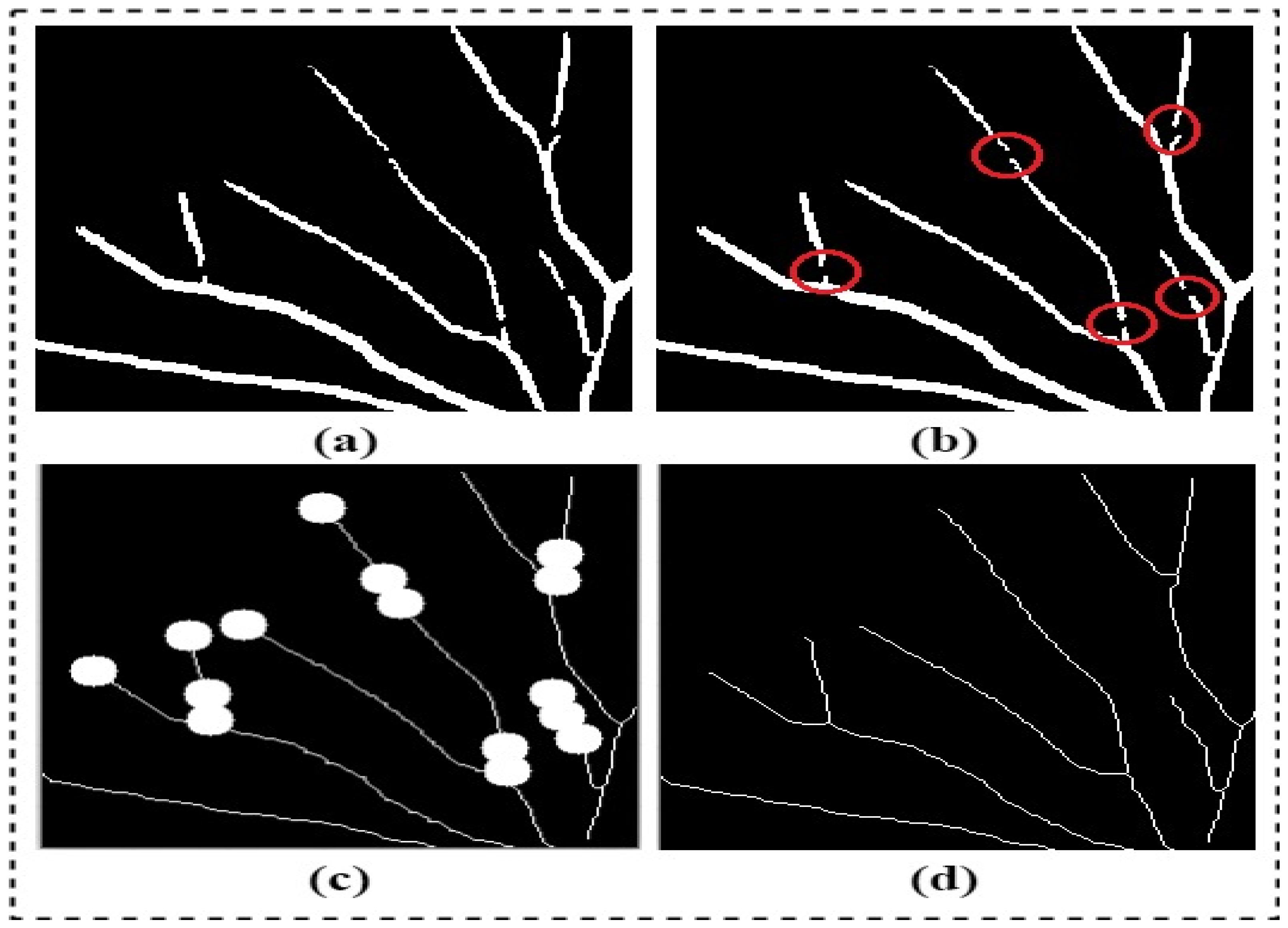
Once the segmented retinal image is obtained from the trainable filter, the output is used to produce the final segmented image. Then, a novel blood vessel linking procedure was proposed to correctly join the discontinuous blood vessels produced in the segmented image resulting from the previous step. These discontinuous blood vessels are presented in the final segmented image due to the poor visibility of the specific blood vessels or the noise presented in the retinal image. The accuracy of the extract clinical features, such as the tortuosity, length, density, and thickness of blood vessels, can significantly be affected by the appearance of the discontinuous blood vessels. Thus, a new procedure was proposed in this study to correctly connect the discontinuous blood vessels in the final segmented image. The proposed blood vessel linking procedure was implemented as follows:
3.3. Clinical Features Extraction Stage
This method was designed for diagnosing retinopathies diseases, for use by ophthalmologists and eye specialists, which can help shape the retinal lesions’ thickness, length, or presentation. All this is connected with cardiovascular and retinopathies diseases. The quantitative analysis of abnormalities in blood vessel structures can be found in vessel tortuosity. It can describe their severity level and treatment assessments. One of the main aims of this work is to develop an automated algorithm description procedure to analyse the whole blood vessels network in the retinal image. The clinical features extraction stage computes a set of useful clinical features from the automatically detected retinal blood vessels accurately and objectively. In this stage, several clinical features associated with the healthiness of the retinal blood vessels are extracted as follows:
3.3.1. Vessel Length
The length of the retinal blood vessel was computed for each vessel’s segment by firstly taking the vessel’s skeleton structure, and then the distance between sequential pixels in the blood vessel segment is summed as in Equation (14).
Here, N refers to the number of sequential pixels produced from the blood vessel skeleton segment, and () refers to the pixels coordinates in the blood vessel segment.
3.3.2. Vessel Density
The retinal blood vessels density was calculated by dividing the sum of all the pixels of the blood vessels by the overall area of the whole retinal image as in Equation (15):
3.3.3. Vessel Tortuosity
The tortuosity coefficient of the blood vessel is interpreted as a degree of curvature and twists presented in the blood vessel course, as shown in
Figure 7. Some studies have proved that the vessel tortuosity coefficient can be associated with the average internal blood pressure; however, no significant increase was observed until the critical blood pressure level is reached [
17,
18]. Herein, the mean tortuosity coefficient of the whole retinal blood vessels network was computed. First, the skeleton structure of the blood vessels was produced. This was followed by defining the branch points of the blood vessels to divide the length of the Blood Vessel Segment (BVS) into (b) branches, as in Equation (16):
Then, the tortuosity coefficient index for the (
BVS) was then computed as follows:
where
refers to the length of vessel branch, and it was estimated by Equation (17).
is the straightforward distance between the endings point and was estimated as follows:
Here,
N refers to the number of fundamental pixels captured from the branch of the blood vessels, while (
x,
y) refers to the pixels coordinates in each branch of the blood vessels. Finally, the mean tortuosity coefficient of the entire blood vessels network was acquired by calculating the mean tortuosity values obtained of each blood vessel.
3.3.4. Vessel Thickness
The blood vessel thickness is the average width of the retinal blood vessels. In this paper, a new procedure for computing the retinal blood vessels thickness is developed.
Figure 8 shows the output of the developed thickness procedure. The primary steps of the developed procedure after identifying each blood vessel were implemented as follows:
Distance transform was computed from the binary image of the detected retinal blood vessels, where all background pixels in the transformed image become white, while the object pixels become black. This transform calculates the Euclidean distance for each black pixel in the segmented image to the nearest non-zero pixel. In the developed procedure, the distance transform was implemented on the inverse of the binary image of the detected retinal blood vessels. Thus, for each pixel of the detected blood vessel, the Euclidean distance of that specific pixel to the nearest border pixel of the blood vessel was calculated.
After applying the distance transform, the blood vessel pixels that have the most significant distance values in the distance transform will be located at the middle of the blood vessel segment. The distance values representing the halfway edge between the blood vessel segment were obtained with some leniency of the most significant distance values because of the floating-point computation.
Finally, the overall average of all accumulated distance values defines the half-width of the blood vessel. Consequently, the blood vessel thickness (width) was measured by multiplying the outcome reached by two.
4. Experimental Results and Discussion
To evaluate the performance and accuracy of the developed hybrid and fully automated segmentation algorithm, for detecting the retinal blood vessels, we used two extremely challenging fundus images datasets, namely, DRIVE [
20] and High-Resolution Fundus (HRF) [
21]. In this study, several extensive experiments were conducted. Firstly, the main description of the employed retinal images datasets in these experiments is given. Secondly, a detailed evaluation of the fully automated segmentation algorithm (a trainable filtering algorithm) is presented along with their combination and compared their performance against the Ground Truth (GT) images. Finally, the performance of the developed algorithms is compared with the state-of-the-art approaches.
4.1. Dataset Description
The performance of the proposed blood vessel segmentation algorithms has been tested using two established, publicly available datasets of retinal fundus images (DRIVE and HRF). These two datasets have gained particular popularity because they provide the associated GT images in which different expert observers manually detect the blood vessel. Thus, they enable the possibility of comparing the results obtained against the provided GT images to validate the reliability and efficiency of the proposed algorithms. The main aim of these two datasets is to establish and encourage comparative studies on developing automated segmentation algorithms for retinal blood vessels in the fundus images.
1. DRIVE dataset [
20]: This dataset comprises 40 coloured retinal images split into a training set and a testing set, each of which comprises 20 images. The mask image representing the Field-Of-View (FOV) of the retina area is provided for each image and the corresponding GT image. One expert manually segmented the blood vessels in the retinal images of the training set. In this work, the training set was used to fine-tune the parameters of the proposed segmentation algorithms. On the other hand, two other experts manually segmented the blood vessels in the testing set images. The actual performance of the proposed vessel segmentation algorithms was assessed using the testing set. The DRIVE database contains retinal images captured from 400 diabetic subjects between 25–90 years old in the Netherlands. Around 40 images were randomly chosen: 33 images without any sign of diabetic retinopathy, and seven images showed mild early diabetic retinopathy. The retinal images were captured using a Canon CR5 non-mydriatic 3CCD camera with a 45° FOV. All the images were saved in TIF format with an 8-bits coloured image and size of 768 × 584 pixels. An example of retinal fundus images from the DRIVE dataset with corresponding manually gold standard images is shown in
Figure 9.
2. HRF dataset [
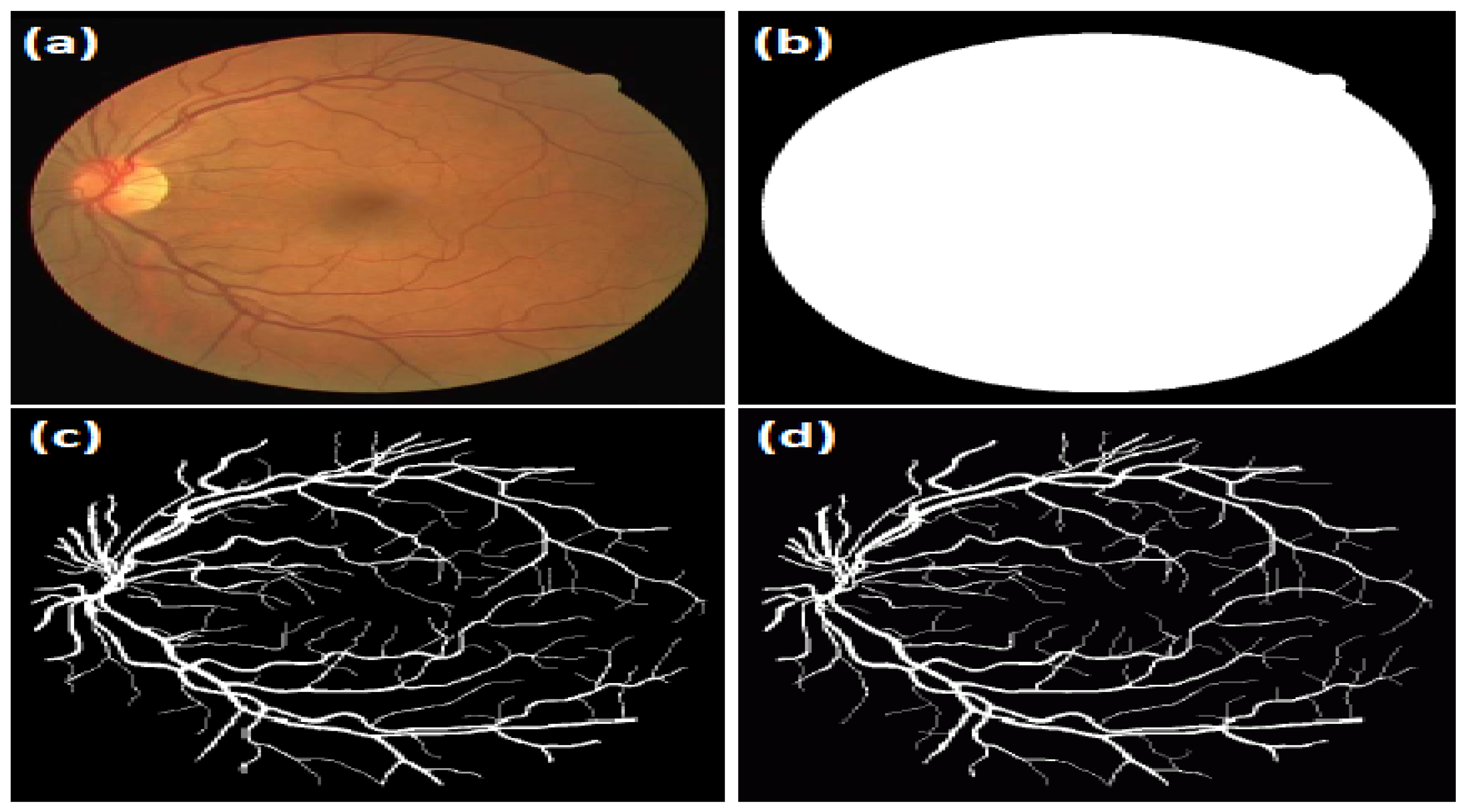
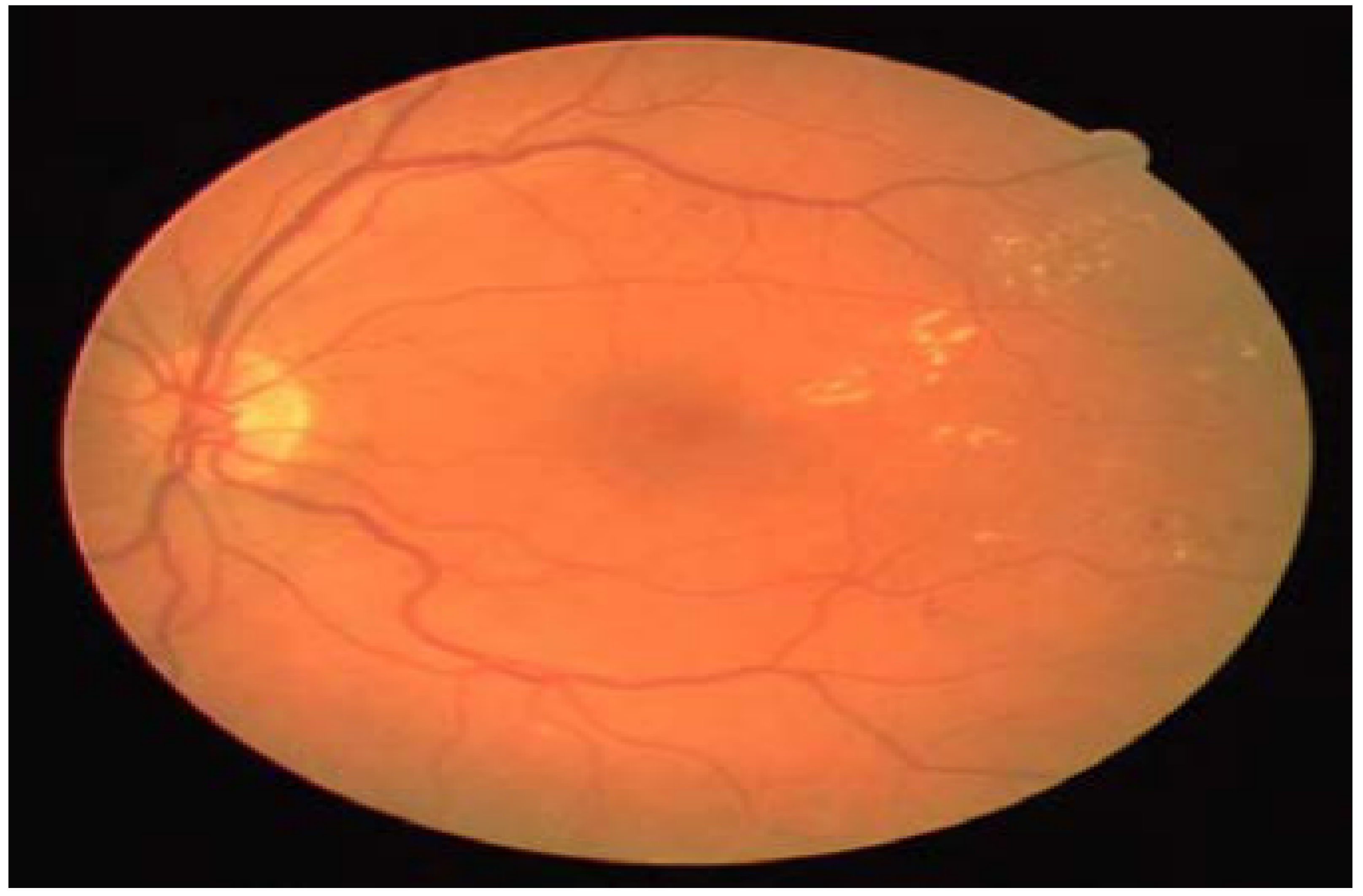
21]: The HRF dataset comprises 45 images captured from three different groups (e.g., healthy subjects, diabetic retinopathy patients, and glaucomatous patients). Each group has 15 images acquired using a mydriatic fundus CANON CF-60UVi camera with a 60° FOV. All the images were saved in JPEG format with a 24-bits coloured image and size of 3504 × 2336 pixels and a pixel size of 6.05 × 6.46 μm. The binary FOV-mask images of the dataset are provided to perform the analysis only in the region surrounded by the dark background (see
Figure 10b). In this dataset, the tree of blood vessels was manually traced by three experts in retinal image interpretation. An example of retinal fundus images from the HRF dataset with corresponding manually gold standard images is shown in
Figure 10.
4.2. Blood Vessel Segmentation Evaluation
In the binary classification task, each pixel in the input image is classified as a vessel by the proposed algorithm. It is also classified as a vessel in the GT image, counted as a true positive. On the other hand, each pixel is classified as a vessel in the final segmented image, but not in the GT image, counted as a false positive (see
Table 1). In the evaluation of the retinal vessel segmentation, the average values of five quantitative performance measures were calculated to validate the efficiency of the proposed algorithms, including the Accuracy (Acc.), Sensitivity (Sen.), Specificity (Spe.), Positive Predictive Value (PPV), and Negative Predictive Value (NPV). These five quantitative measures are computed as follows:
Here, TP, TN, FP, and FN refer to True Positives, True Negatives, False Positives, and False Negatives, respectively. The Acc. measurement refers to the total number of correctly classified pixels to the number of pixels in the FOV-mask image. Sensitivity (Sen.) refers to the ability of the proposed algorithm to detect the vessel pixels correctly. Specificity (Spe.) is the ability of the proposed algorithm to detect non-vessel pixels correctly. The PPV or Precision rate refers to the ratio of pixels correctly identified as vessel pixels. Finally, the NPV is the ratio of pixels correctly identified as non-vessel pixels (e.g., background).
4.3. Results on DRIVE Dataset
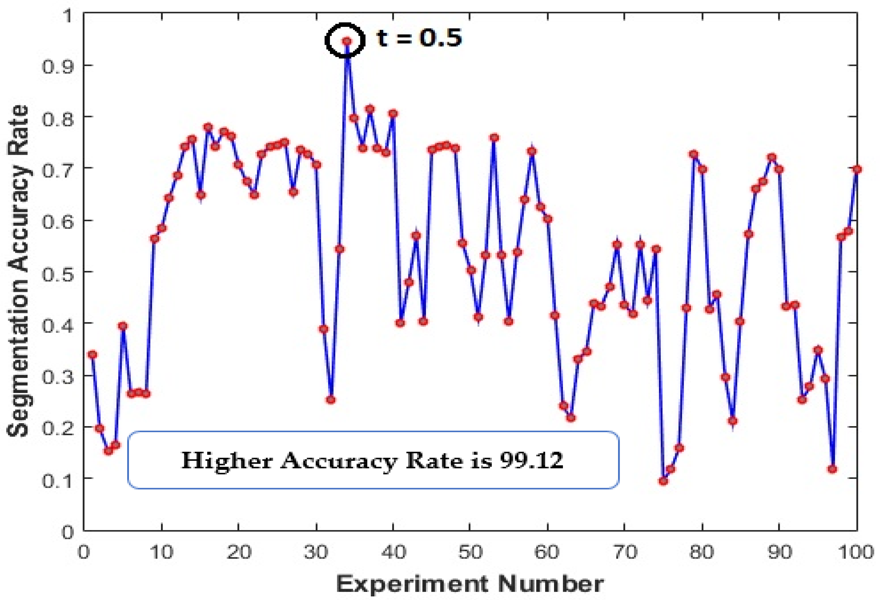
Firstly, the performance of the proposed algorithm for detecting the retinal blood vessels was evaluated on the DRIVE dataset. Training set images were used, and several extensive experiments were carried out to choose the best value for a set of parameters in such a way as to maximize the segmentation accuracy of the proposed algorithms. For instance, the value of the parameter (
t) (in Equation (13) using the proposed trainable filters algorithm was chosen by varying its value between 0 and 1 in steps of 0.01. This threshold process assigns each pixel into two labels: Vessels and Non-Vessels. Then, the segmentation accuracy was computed to select the best value of the parameter (
t). As shown in
Figure 11, the best value of parameter (
t) was set to 0.5. Hence, 100 experiments were carried out where we increased the value of the parameter (t) by 0.1. In the evaluation stage, five performance evaluation metrics were computed using the testing images, and the two provided human observers as the GT images.
Table 2 shows the results generated using the proposed trainable filters algorithm. This table shows that better results have been achieved using the second human observer than the first human observer in terms of all the adopted five evaluation metrics. It achieved an Acc. of 99.12%, Sen. of 98.89%, Spe. of 98.86%, PPV of 93.28%, and NPV of 97.77%. Furthermore, the performance of the proposed trainable filters algorithm has outperformed the performance of the proposed algorithm by achieving an overall average Acc. of 98.785%, Sen. of 98.455%, Spe. of 98.375%, PPV of 92.125%, and NPV of 95.93%. Then, the proposed blood vessel linking procedure was applied to correctly join the discontinuous blood vessels produced in the segmented retinal image resulting from the previous step. In this work, to validate the advantage of applying the proposed blood vessel linking procedure, the adopted five evaluation metrics were computed with and without applying the proposed blood vessel linking procedure. An example of the output segmentation results on the DRIVE dataset is shown in
Figure 12.
In this work, the performance of the proposed algorithms was compared with current state-of-the-art vessel segmentation approaches on the DRIVE dataset images. The results obtained from the second human observer have been considered for comparison purposes. It was noted that most previously published approaches in the literature report the values of accuracy, sensitivity, and specificity. Thus, the overall average of these three metrics and the PPV and NPV values have been computed with GT images (2nd human observer) and listed in
Table 3. Although, Li et al. [
22], Jin et al. [
23], Hassan et al. [
24], Dasgupta and Singh [
25], Li et al. [
26], Tamim et al. [
27], Yang et al. [
28], and Yang et al. [
29] have achieved a higher Spe. and NPV value compared with the proposed trainable filters algorithm in terms of all the adopted five evaluation metrics, better results were obtained using the proposed algorithm mentioned earlier, except for Yang et al. [
28], which achieved slightly a higher NPV value.
4.4. Results on HRF Dataset
In this section, the performance of the proposed vessels segmentation algorithm has been assessed using the HRF dataset using the same parameter configuration described in
Section 4.2. The adopted five evaluation metrics were initially calculated for the proposed vessels segmentation algorithms using the GT images provided in the HRF dataset, as shown in
Table 4. A comparable performance was achieved by the proposed trainable filtering, with a PPV of 95.89% and NPV of 98.97%. On the other hand, a better Acc. of 98.78%, Sen. of 99.12%, and Spe. of 99.34% was obtained using the proposed algorithm. An example of the output segmentation results on the HRF dataset is shown in
Figure 13.
The performance of the proposed blood vessel segmentation algorithms has also been compared with the state-of-the-art approaches on the HRF dataset, as given in
Table 5. It was observed that some existing approaches have achieved a slightly higher segmentation accuracy compared with the proposed algorithms. For instance, Kishorea and Ananthamoorthy [
34] have reached an Acc. of 99.6% compared to an Acc. of 98.76% and 98.78 using the proposed trainable filters algorithm. However, the work presented in [
34] has obtained inferior results in another evaluation metric (e.g., Sen., Spe., PPV, and NPV) compared with the proposed algorithm. On the other hand, Chalakkal et al. [
37] has achieved a slightly better Spe. value of 100% compared with Spe. values of 99.17%, 99.35%, and 99.78%, using the trainable filters. However, they got inferior results on the other evaluation metric (e.g., Acc. and Sen.). Finally, one can see the best Sen. values of 98.87%, 99.12%, and 99.89% were obtained using the trainable filtering algorithm, compared with the state-of-the-art approaches on the HRF dataset.
The first human observer of the DRIVE dataset: Pearson correlation plots were also adopted to confirm further the clinical reliability and usefulness of the proposed blood vessels segmentation algorithms as effective tools to provide a precise and automated estimation of the vessel’s clinical features. As shown in
Figure 13, a Pearson’s correlation r and p coefficient of r = 0.81,
p < 0.0001, for vessel tortuosity; r = 0.87,
p < 0.0001, for vessel thickness; r = 0.76,
p < 0.0001, for vessel length; and r = 0.93,
p < 0.0001, for vessel density using the proposed trainable filters algorithm (see
Figure 14).
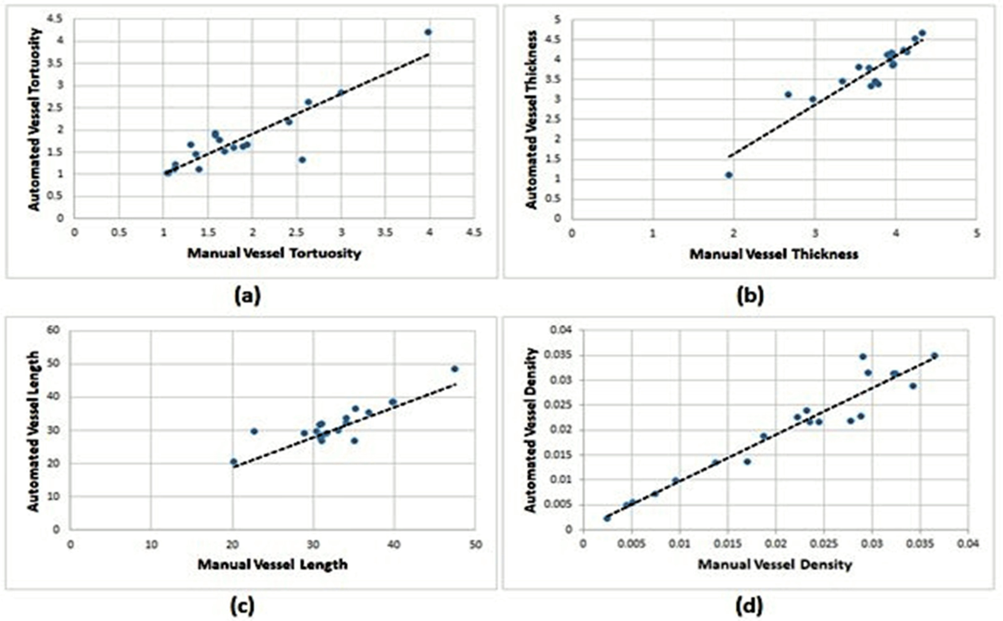
The same clinical evaluation was carried out to get the automated estimation of the clinical features from the DRIVE dataset using the 2nd human observer. As shown in
Table 6 and
Figure 14, a Pearson’s correlation r and p coefficient of r = 0.88,
p < 0.0001 were achieved for vessel tortuosity; r = 0.87,
p < 0.0001, for vessel thickness; r = 0.96,
p < 0.0001, for vessel length; and r = 0.94,
p < 0.0001, for vessel density using the proposed trainable filters algorithm (see
Figure 15).
Further evaluation was performed on the HRF Dataset, which contains 40 GT images constructed to efficiently assess the performance of the proposed blood vessel segmentation algorithms.
Table 7 shows the overall AV., STD, Max, and Min of each clinical feature. The manual and automated images were computed along with the Diff and Diff % between them. The average Diff % between the manual and automated estimations calculated using the proposed trainable filter algorithm were 2.560%, 12.59%, 2.484%, and 5.529% for tortuosity, thickness, length, and density, respectively. Correlation plots between the manual and automated clinical estimations from the HRF dataset using the proposed trainable filtering algorithm are presented in
Figure 16.
5. Conclusions
This study proposes an accurate, rapid, and fully automatic blood vessel segmentation and clinical features measurement algorithm for retinal fundus images. The proposed algorithm comprises two primary stages: the blood vessel segmentation and clinical features extraction stages. In the blood vessel segmentation stage, a fully automated segmentation algorithm was proposed and named a trainable filters algorithm to detect the blood vessels in the retinal fundus images accurately. The current algorithm has an image enhancement pre-processing procedure to address the problems of blurring, uneven lighting, and low contrast of the retinal fundus image, and promotes the early diagnosis of several eye pathologies. Several comprehensive experiments were carried out to assess the performance of the developed fully automated segmentation algorithm in detecting the retinal blood vessels using two extremely challenging fundus images datasets, namely, the DRIVE and HRF datasets. Initially, the accuracy of the developed algorithm was evaluated in terms of adequately detecting the retinal blood vessels. In these experiments, five quantitative performance measures were calculated to validate the efficiency of the proposed algorithm, including the Acc., Sen., Spe., PPV, and NPV measures, and compared with current state-of-the-art vessel segmentation approaches on the DRIVE dataset. The results obtained showed a significant improvement by achieving an Acc., Sen., Spe., PPV, and NPV of 99.55%, 99.93%, 99.09%, 93.45%, and 98.89, respectively. Then, the efficiency and reliability of the proposed algorithm in extracting valuable and helpful clinical features were also evaluated by conducting extensive experiments. Statistically notable correlations between the manual and automated estimations of the adopted four clinical features were obtained using the proposed algorithm on both datasets (DRIVE and HRF). We would like to advise researchers to focus on multi-scale methods and try to combine these with our proposed algorithm due to the high quality of the results we produced in the segmentation domain.
Author Contributions
Conceptualization, A.A.A. and M.A.M. (Moamin A. Mahmoud).; methodology, A.A.A.; software, A.A.A.; validation, H.A., S.S.G. and M.A.M. (Mazin Abed Mohammed); formal analysis, A.A.A.; investigation, M.A.M. (Mazin Abed Mohammed); resources, H.A.; data curation, S.S.G.; writing—original draft preparation, A.A.A. and M.A.M. (Moamin A. Mahmoud); writing—review and editing, M.A.M. (Mazin Abed Mohammed); supervision, M.A.M. (Moamin A. Mahmoudand) and M.A.M. (Mazin Abed Mohammed); project administration, M.A.M. (Moamin A. Mahmoud) and M.A.M. (Mazin Abed Mohammed); funding acquisition, H.A. All authors have read and agreed to the published version of the manuscript.
Funding
This work is sponsored by Universiti Tenaga Nasional (UNITEN) under the Bold Re-search Grant Scheme No. J510050002.
Conflicts of Interest
The authors declare no conflict of interest.
References
- Abdulsahib1, A.A.; Mahmoud, M.A.; Mohammed, M.A.; Rasheed, H.H.; Mostafa, S.A.; Maashi, M.S. Comprehensive Review of Retinal Blood Vessels Segmentation and Classification Techniques Intelligent Solutions for Green Computing in Medical Images, Current Challenges, Open issues, and Knowledge Gaps in Fundus Medical Images. Netw. Model. Anal. Health Inform. Bioinform. 2021, 10, 20. [Google Scholar] [CrossRef]
- Lal, S.; Rehman, S.U.; Shah, J.H.; Meraj, T.; Rauf, H.T.; Damaševičius, R.; Mohammed, M.A.; Abdulkareem, K.H. Adversarial Attack and Defence through Adversarial Training and Feature Fusion for Diabetic Retinopathy Recognition. Sensors 2021, 21, 3922. [Google Scholar] [CrossRef] [PubMed]
- Balasubramanian, K.; Ananthamoorthy, N.P. Robust retinal blood vessel segmentation using convolutional neural network and support vector machine. J. Ambient. Intell. Humaniz. Comput. 2019, 12, 3559–3569. [Google Scholar] [CrossRef]
- Boudegga, H.; Elloumi, Y.; Akil, M.; Bedoui, M.H.; Kachouri, R.; Ben Abdallah, A. Fast and efficient retinal blood vessel segmentation method based on deep learning network. Comput. Med. Imaging Graph. 2021, 90, 101902. [Google Scholar] [CrossRef] [PubMed]
- Ramos-Soto, O.; Rodríguez-Esparza, E.; Balderas-Mata, S.E.; Oliva, D.; Hassanien, A.E.; Meleppat, R.K.; Zawadzki, R.J. An efficient retinal blood vessel segmentation in eye fundus images by using optimized top-hat and homomorphic filtering. Comput. Methods Programs Biomed. 2021, 201, 105949. [Google Scholar] [CrossRef]
- Ramos-Soto, O.; Rodríguez-Esparza, E.; Balderas-Mata, S.E.; Oliva, D.; Hassanien, A.E.; Meleppat, R.K.; Zawadzki, R.J. Quantification of malaria parasitaemia using trainable semantic segmentation and capsnet. Pattern Recognit. Lett. 2020, 138, 88–94. [Google Scholar]
- Zebari, D.A.; Zeebaree, D.Q.; Abdulazeez, A.M.; Haron, H.; Hamed, H.N.A. Improved Threshold Based and Trainable Fully Automated Segmentation for Breast Cancer Boundary and Pectoral Muscle in Mammogram Images. IEEE Access 2020, 8, 203097–203116. [Google Scholar] [CrossRef]
- Tarasiewicz, T.; Nalepa, J.; Kawulok, M. Skinny: A lightweight u-net for skin detection and segmentation. In Proceedings of the 2020 IEEE International Conference on Image Processing (ICIP), Abu Dhabi, United Arab Emirates, 25–28 October 2020. [Google Scholar]
- Lakshmi, P.V.; NidhiBartakke, P.; Rao, P.S.; Rao, G.A.V.R.C.; Srikanth, D. Diagnosis of diabetic retinopathy with transfer learning from deep convolutional neural network. J. Crit. Rev. 2020, 7, 2232–2239. [Google Scholar]
- Soaibuzzaman, P.D.W.H. Image Segmentation Based on Convolutional Neural Networks; Seminar Report 2021; Technische Universty Chemnitz: Chemnitz, Germany, 2021. [Google Scholar]
- Hatamizadeh, A.; Sengupta, D.; Terzopoulos, D. End-to-End Trainable Deep Active Contour Models for Automated Image Segmentation: Delineating Buildings in Aerial Imagery. In European Conference on Computer Vision; Computer Science Department, University of California: Los Angeles, CA, USA, 2020. [Google Scholar]
- Chiu, C.-C.; Ting, C.-C. Contrast Enhancement Algorithm Based on Gap Adjustment for Histogram Equalization. Sensors 2016, 16, 936. [Google Scholar] [CrossRef] [Green Version]
- Dorothy, R.; Joany, R.M.; Rathish, R.J.; Prabha, S.S.; Rajendran, S.; Joseph, S. Image enhancement by Histogram equalization. Int. J. Nano Corr. Sci. Eng. 2015, 2, 21–30. [Google Scholar]
- Reza, A.M. Realization of the Contrast Limited Adaptive Histogram Equalization (CLAHE) for Real-Time Image Enhancement. J. VLSI Signal Process. 2004, 38, 35–44. [Google Scholar] [CrossRef]
- Min, B.S.; Lim, D.K.; Kim, S.J.; Lee, J.H. A Novel Method of Determining Parameters of CLAHE Based on Image Entropy. Int. J. Softw. Eng. Appl. 2013, 7, 113–120. [Google Scholar] [CrossRef] [Green Version]
- Raj, V.N.P.; Venkateswarlu, T. Denoising of Medical Images Using Dual Tree Complex Wavelet Transform. Procedia Technol. 2012, 4, 238–244. [Google Scholar] [CrossRef] [Green Version]
- Kylstra, J.A.; Wierzbicki, T.; Wolbarsht, M.L.; Landers, M., III; Stefansson, E. The relationship between retinal vessel tortuosity, diameter, and transmural pressure. Graefe’s Arch. Clin. Exp. Ophthalmol. 1986, 224, 477–480. [Google Scholar] [CrossRef]
- Patasius, M.; Marozas, V.; Lukosevicius, A.; Jegelevicius, D. Model based investigation of retinal vessel tortuosity as a function of blood pressure preliminary results. In Proceedings of the 29th Annual International Conference of the IEEE EMBS Cité Internationale, Lyon, France, 23–26 August 2007. [Google Scholar]
- Joshi, V.S. Analysis of Retinal Vessel Networks Using Quantitative Descriptors of Vascular Morphology. Ph.D. Thesis, The University of Iowa, Iowa City, IA, USA, 2012. [Google Scholar]
- Korotkova, O.; Salem, M.; Dogariu, A.; Wolf, E. Changes in the polarization ellipse of random electromagnetic beams propagating through the turbulent atmosphere. Waves Random Complex Media 2005, 15, 353–364. [Google Scholar] [CrossRef]
- Odstrcilik, J.; Kolar, R.; Budai, A.; Hornegger, J.; Jan, J.; Gazarek, J.; Kubena, T.; Cernosek, P.; Svoboda, O.; Angelopoulou, E. Retinal vessel segmentation by improved matched filtering: Evaluation on a new high-resolution fundus image database. IET Image Process. 2013, 7, 373–383. [Google Scholar] [CrossRef]
- Li, Q.; Feng, B.; Xie, L.; Liang, P.; Zhang, H.; Wang, T. A Cross-Modality Learning Approach for Vessel Segmentation in Retinal Images. IEEE Trans. Med. Imaging 2015, 35, 109–118. [Google Scholar] [CrossRef]
- Al-Waisy, A.S.; Qahwaji, R.; Ipson, S.; Al-Fahdawi, S. A multimodal deep learning framework using local feature representations for face recognition. Mach. Vis. Appl. 2017, 29, 35–54. [Google Scholar] [CrossRef] [Green Version]
- Hassan, G.; El-Bendary, N.; Hassanien, A.E.; Fahmy, A.; Snasel, V. Retinal Blood Vessel Segmentation Approach Based on Mathematical Morphology. Procedia Comput. Sci. 2015, 65, 612–622. [Google Scholar] [CrossRef] [Green Version]
- Dasgupta, A.; Singh, S. A fully convolutional neural network based structured prediction approach towards the retinal vessel segmentation. In Proceedings of the 14th International Symposium on Biomedical Imaging (ISBI), Melbourne, VIC, Australia, 18–21 April 2017; pp. 248–251. [Google Scholar] [CrossRef] [Green Version]
- Li, L.; Verma, M.; Nakashima, Y.; Nagahara, H.; Kawasaki, R. IterNet: Retinal image segmentation utilizing structural redundancy in vessel networks. In Proceedings of the 2020 IEEE Winter Conference on Applications of Computer Vision, WACV 2020, Snowmass, CO, USA, 1−5 March 2020; pp. 3645–3654. [Google Scholar] [CrossRef]
- Tamim, N.; Elshrkawey, M.; Azim, G.A.; Nassar, H. Retinal Blood Vessel Segmentation Using Hybrid Features and Multi-Layer Perceptron Neural Networks. Symmetry 2020, 12, 894. [Google Scholar] [CrossRef]
- Yang, J.; Huang, M.; Fu, J.; Lou, C.; Feng, C. Frangi based multi-scale level sets for retinal vascular segmentation. Comput. Methods Programs Biomed. 2020, 197, 105752. [Google Scholar] [CrossRef] [PubMed]
- Yang, Y.; Shao, F.; Fu, Z.; Fu, R. Blood vessel segmentation of fundus images via cross-modality dictionary learning. Appl. Opt. 2018, 57, 7287–7295. [Google Scholar] [CrossRef]
- De, I.; Chanda, B.; Chattopadhyay, B. Enhancing effective depth-of-field by image fusion using mathematical morphology. Image Vis. Comput. 2006, 24, 1278–1287. [Google Scholar] [CrossRef]
- Mukhopadhyay, S.; Chanda, B. Multiscale morphological segmentation of gray-scale images. IEEE Trans. Image Process. 2003, 12, 533–549. [Google Scholar] [CrossRef] [Green Version]
- Christodoulidis, A.; Hurtut, T.; Tahar, H.B.; Cheriet, F. A Multi-scale Tensor Voting Approach for Small Retinal Vessel Segmentation in High Resolution Fundus Images. Comput. Med. Imaging Graph. 2016, 52, 28–43. [Google Scholar] [CrossRef] [PubMed]
- Samuel, P.M.; Veeramalai, T. Multilevel and Multiscale Deep Neural Network for Retinal Blood Vessel Segmentation. Symmetry 2019, 11, 946. [Google Scholar] [CrossRef] [Green Version]
- Kishore, B.; Ananthamoorthy, N. Glaucoma classification based on intra-class and extra-class discriminative correlation and consensus ensemble classifier. Genomics 2020, 112, 3089–3096. [Google Scholar] [CrossRef] [PubMed]
- Yang, Y.; Shao, F.; Fu, Z.; Fu, R. Discriminative dictionary learning for retinal vessel segmentation using fusion of multiple features. Signal Image Video Process. 2019, 13, 1529–1537. [Google Scholar] [CrossRef]
- Keerthiveena, B.; Esakkirajan, S.; Selvakumar, K.; Yogesh, T. Computer-aided diagnosis of retinal diseases using multidomain feature fusion. Int. J. Imaging Syst. Technol. 2019, 30, 367–379. [Google Scholar] [CrossRef]
- Vostatek, P. Blood Vessel Segmentation in the Analysis of Retinal and Diaphragm Images Blood Vessel Segmentation in the Analysis of Retinal and Diaphragm. Ph.D. Thesis, Faculty of Electrical Engineering, Prague, Czech Republic, 2017. [Google Scholar]
Figure 1.
Block diagram of the proposed blood vessel segmentation and clinical features measurement algorithm.
Figure 1.
Block diagram of the proposed blood vessel segmentation and clinical features measurement algorithm.
Figure 2.
The fundamental stages of the proposed trainable filtering algorithm for detecting the retinal blood vessels.
Figure 2.
The fundamental stages of the proposed trainable filtering algorithm for detecting the retinal blood vessels.
Figure 3.
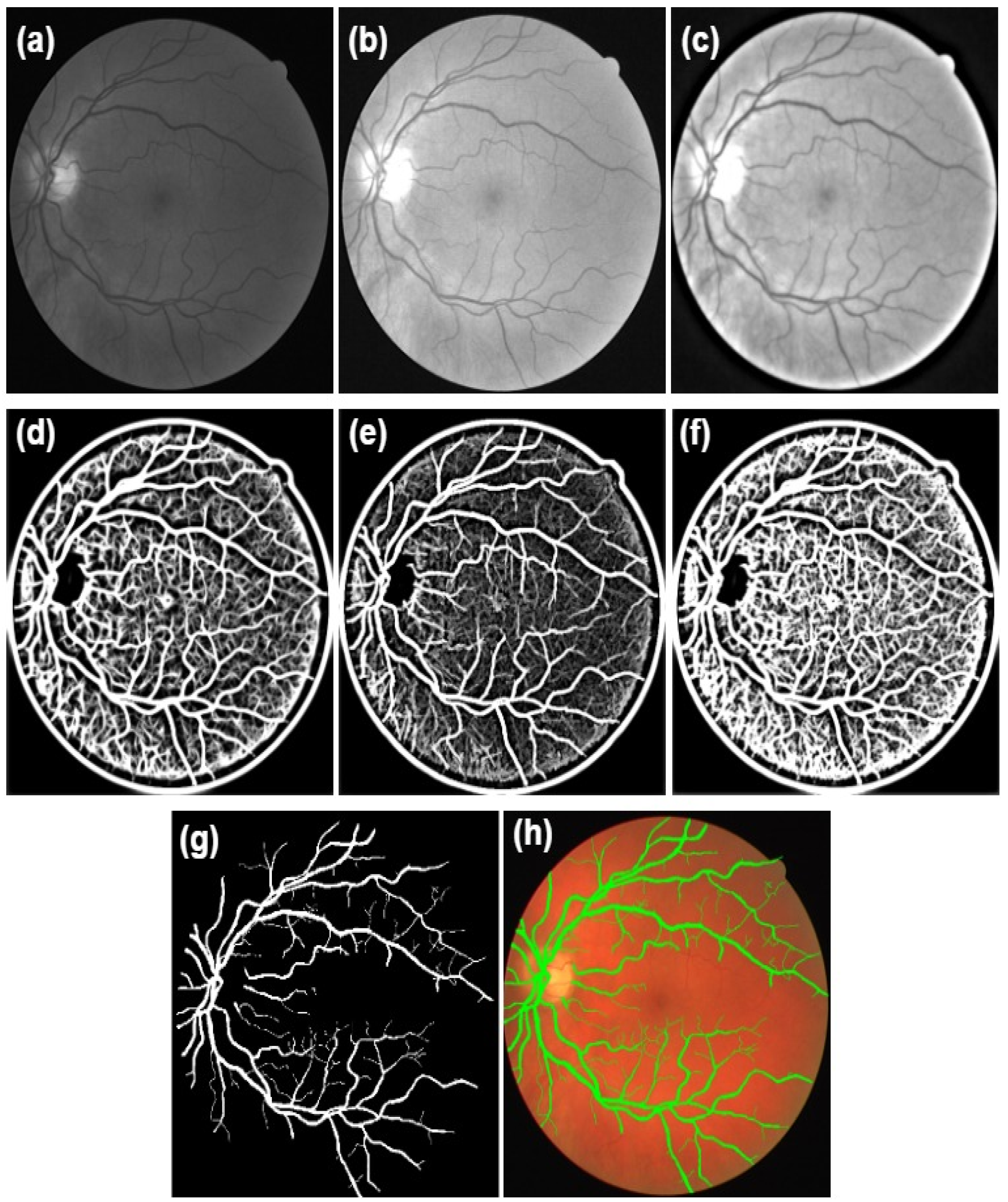
The proposed trainable filters algorithm outputs: (a) the normalized green channel; (b) the CLAHE output; (c) the DT-CWT output; (d) the output of the symmetric filter; (e) the output of the asymmetric filter; (f) the combination of the symmetric filter and asymmetric filter; (g) the final segmented image from the edge detection stage after applying thresholding; (h) the overlapped automated segmented image with the original retinal image.
Figure 3.
The proposed trainable filters algorithm outputs: (a) the normalized green channel; (b) the CLAHE output; (c) the DT-CWT output; (d) the output of the symmetric filter; (e) the output of the asymmetric filter; (f) the combination of the symmetric filter and asymmetric filter; (g) the final segmented image from the edge detection stage after applying thresholding; (h) the overlapped automated segmented image with the original retinal image.
Figure 4.
(a) DoG responses display the contours of each response; and (b) the representation of the blood vessel as a straight line and recognizing the five points to design the SRF filters.
Figure 4.
(a) DoG responses display the contours of each response; and (b) the representation of the blood vessel as a straight line and recognizing the five points to design the SRF filters.
Figure 5.
The types of detected patterns: (a) line-like pattern; (b) half line-like pattern; and (c) combinations of the created DoG filter to produce the five blobs for the SRF filters.
Figure 5.
The types of detected patterns: (a) line-like pattern; (b) half line-like pattern; and (c) combinations of the created DoG filter to produce the five blobs for the SRF filters.
Figure 6.
The proposed blood vessel linking procedure: (a) the segmented blood vessel structures; (b) the disconnected blood vessels marked in the red circles; (c) the binary circular-shaped structural elements are drawn at the ends of each blood vessel segment; and (d) the resulting image with linked blood vessels.
Figure 7.
An example of severe retinal blood vessel tortuosity in a patient with severe non-proliferative (NPDR) disease [
19].
Figure 7.
An example of severe retinal blood vessel tortuosity in a patient with severe non-proliferative (NPDR) disease [
19].
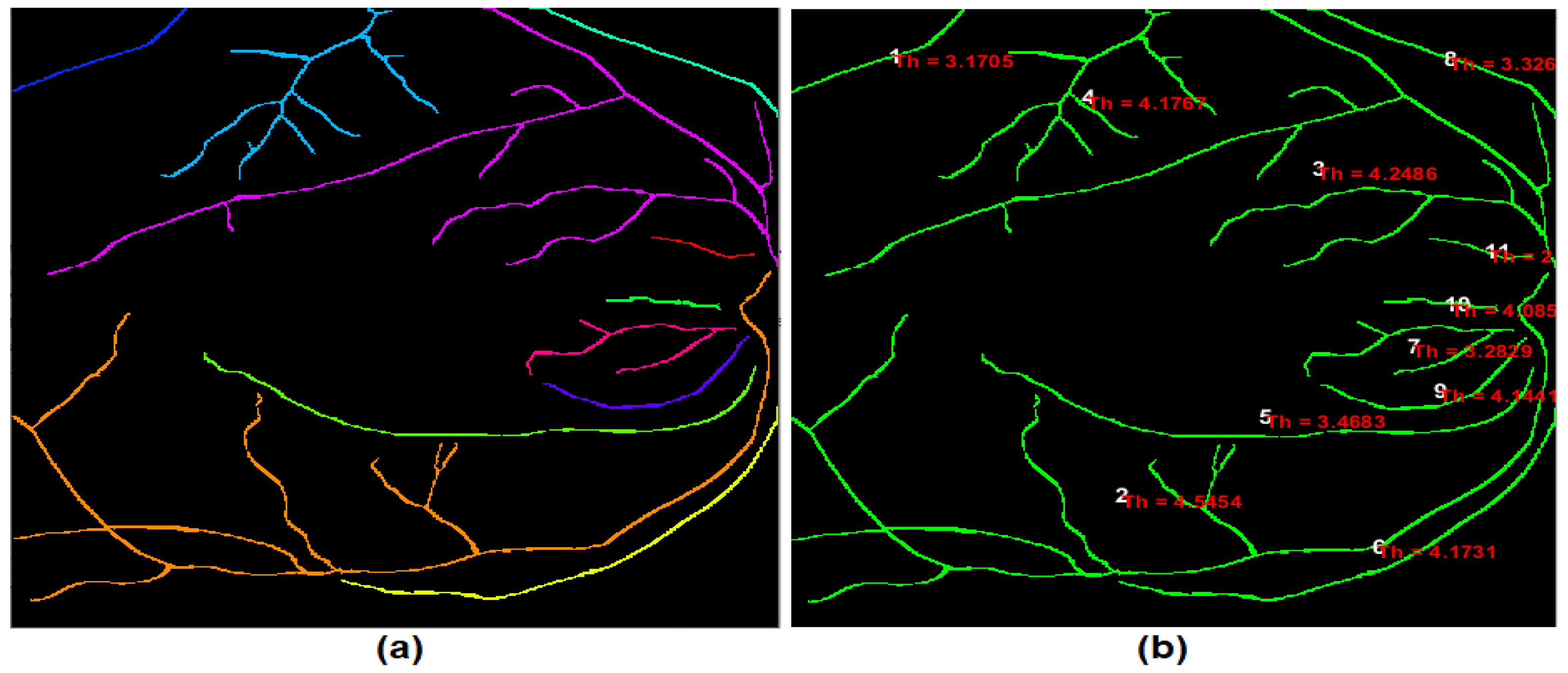
Figure 8.
The output of the developed thickness procedure: (a) coloured labelled retinal blood vessels; and (b) image map for the retinal blood vessels along with their indexes and average thickness values.
Figure 8.
The output of the developed thickness procedure: (a) coloured labelled retinal blood vessels; and (b) image map for the retinal blood vessels along with their indexes and average thickness values.
Figure 9.
Image example from the DRIVE dataset: (a) the original image; (b) FOV-mask image; (c) the manually segmented image of the first expert; and (d) the manually segmented image of the second expert.
Figure 9.
Image example from the DRIVE dataset: (a) the original image; (b) FOV-mask image; (c) the manually segmented image of the first expert; and (d) the manually segmented image of the second expert.
Figure 10.
Image example from the HRF dataset: (a) the original image; (b) FOV-mask image; and (c) the manually segmented image of the expert.
Figure 10.
Image example from the HRF dataset: (a) the original image; (b) FOV-mask image; and (c) the manually segmented image of the expert.
Figure 11.
The segmentation accuracy obtained during 100 experiments to find the best value of the parameter (t) in the using the proposed trainable filters algorithm.
Figure 11.
The segmentation accuracy obtained during 100 experiments to find the best value of the parameter (t) in the using the proposed trainable filters algorithm.
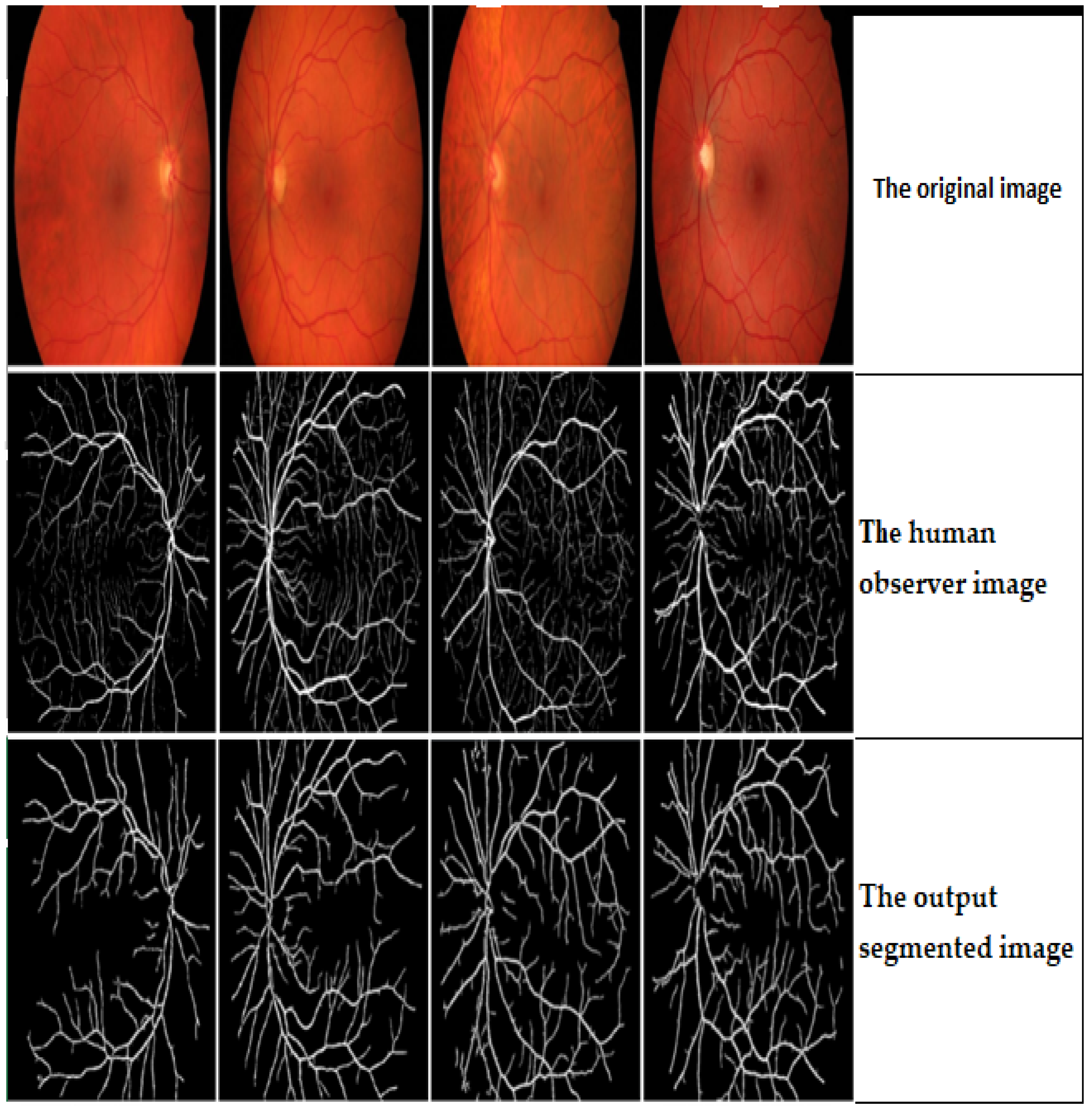
Figure 12.
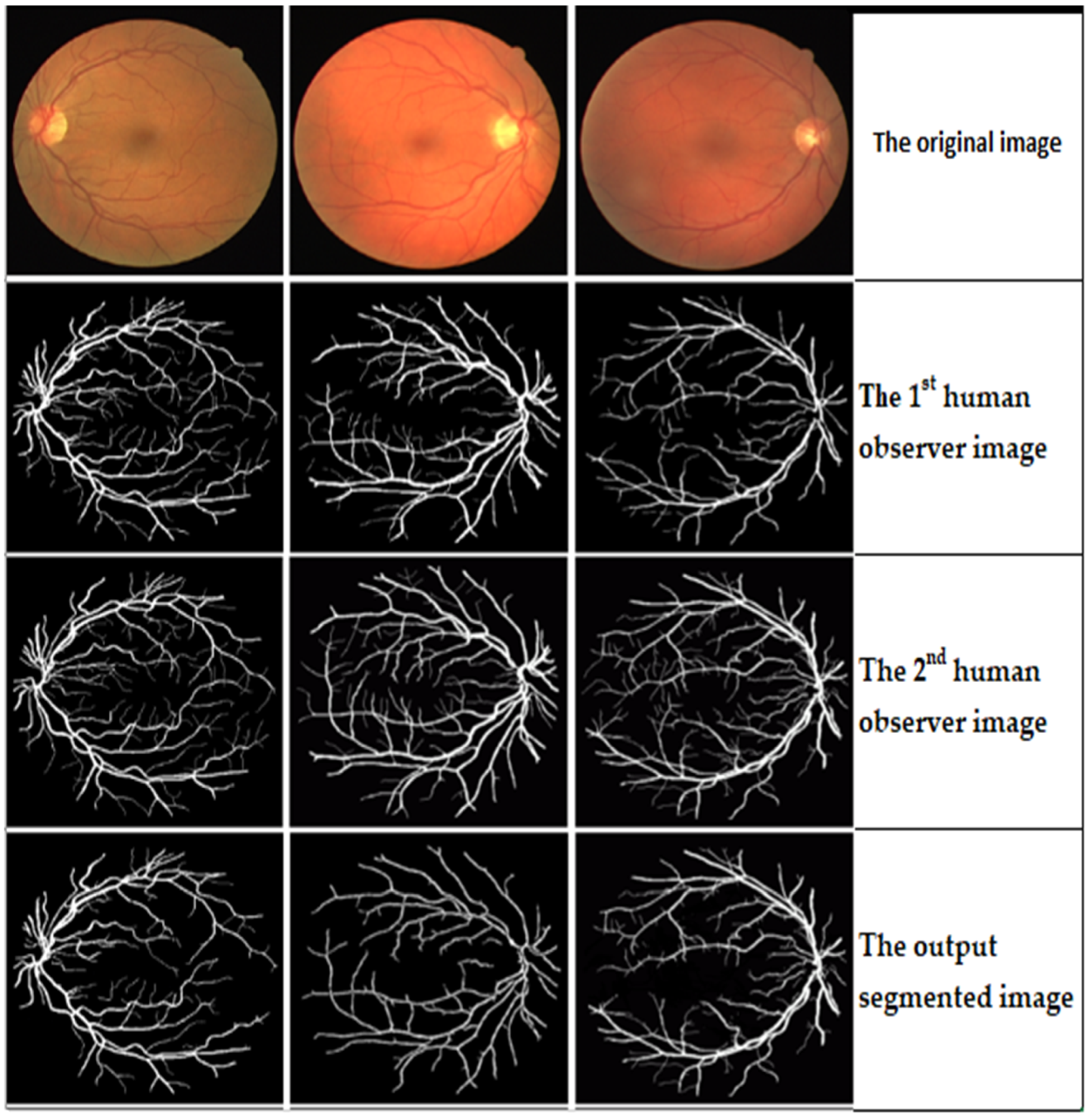
The output segmentation results of the proposed trainable filtering algorithm on the DRVIE dataset.
Figure 12.
The output segmentation results of the proposed trainable filtering algorithm on the DRVIE dataset.
Figure 13.
The output segmentation results of the proposed trainable filtering algorithm on the HRF dataset.
Figure 13.
The output segmentation results of the proposed trainable filtering algorithm on the HRF dataset.
Figure 14.
Correlation plots between manual use by the first human observer and automated clinical estimations from the DRIVE dataset using the proposed trainable filters algorithm: (a) tortuosity; (b) thickness; (c) length; and (d) density.
Figure 14.
Correlation plots between manual use by the first human observer and automated clinical estimations from the DRIVE dataset using the proposed trainable filters algorithm: (a) tortuosity; (b) thickness; (c) length; and (d) density.
Figure 15.
Correlation plots between manual use by the second human observer and automated clinical estimations from the DRIVE dataset using the proposed trainable filters algorithm: (a) tortuosity; (b) thickness; (c) length; and (d) density.
Figure 15.
Correlation plots between manual use by the second human observer and automated clinical estimations from the DRIVE dataset using the proposed trainable filters algorithm: (a) tortuosity; (b) thickness; (c) length; and (d) density.
Figure 16.
Correlation plots between the manual and automated clinical estimations for the HRF dataset using the proposed trainable filters algorithm: (a) tortuosity; (b) thickness; (c) length; and (d) density.
Figure 16.
Correlation plots between the manual and automated clinical estimations for the HRF dataset using the proposed trainable filters algorithm: (a) tortuosity; (b) thickness; (c) length; and (d) density.
Table 1.
Confusion matrix along with the adopted evaluation measures.
Table 1.
Confusion matrix along with the adopted evaluation measures.
| | Vessel Present | Vessel Absent |
|---|
| Vessel detected | True positive (TP) | False positive (FP) |
| Vessel not detected | False negative (FN) | True negative (TN) |
Table 2.
The average values of five quantitative performance measures using the proposed trainable filters algorithm on the DRIVE dataset.
Table 2.
The average values of five quantitative performance measures using the proposed trainable filters algorithm on the DRIVE dataset.
| Measurements | 1st Observer | 2nd Observer | Average |
|---|
| Acc. | 98.45 | 99.12 | 98.78 |
| Sen. | 98.02 | 98.89 | 98.45 |
| Spe. | 97.89 | 98.86 | 98.37 |
| PPV | 90.97 | 93.28 | 92.12 |
| NPV | 94.09 | 97.77 | 95.93 |
Table 3.
Performance comparison of the proposed algorithms with state-of-the-art vessel segmentation approaches on the DRIVE dataset.
Table 3.
Performance comparison of the proposed algorithms with state-of-the-art vessel segmentation approaches on the DRIVE dataset.
| Approaches | Acc. | Sen. | Spe. | PPV | NPV |
|---|
| Odstrcilik et al. [30] | 94.73 | 78.07 | 97.12 | - | - |
| Li et al. [31] | 95.27 | 75.69 | 98.16 | - | - |
| Jin et al. [23] | 96.97 | 78.94 | 98.70 | 85.37 | - |
| Hassan et al. [24] | 96.25 | 87.99 | 97.99 | - | - |
| C. Argyrois [32] | 94.79 | 85.06 | 95.82 | - | - |
| Dasgupta and Singh [25] | 95.33 | 76.91 | 98.01 | 84.98 | - |
| Samuel and Veeramalai [33] | 96.01 | 82.20 | 97.35 | - | - |
| Li et al. [26] | 95.73 | 77.35 | 98.38 | - | - |
| Yang et al. [29] | 95.83 | 73.93 | 97.92 | 77.70 | 97.53 |
| Kishorea and Ananthamoorthy [34] | 94.10 | 69.90 | 95.80 | 85.50 | 94.80 |
| Tamim et al. [27] | 96.07 | 75.42 | 98.43 | 86.34 | 96.53 |
| Yang et al. [28] | 95.22 | 71.81 | 97.47 | 89.23 | 98.50 |
| Yang et al. [35] | 94.21 | 75.60 | 96.96 | 78.54 | 96.44 |
| Keerthiveena et al. [36] | 94.71 | 92.7 | 95.6 | 92.49 | 95.70 |
| Trainable Filters Algo. | 99.12 | 98.89 | 98.86 | 93.28 | 97.77 |
Table 4.
Performance comparison of the trainable filter algorithms on the HRF dataset.
Table 4.
Performance comparison of the trainable filter algorithms on the HRF dataset.
| Measurements | Trainable Filters Algo. |
|---|
| Acc. | 98.78 |
| Sen. | 99.12 |
| Spe. | 99.34 |
| PPV | 95.89 |
| NPV | 98.97 |
Table 5.
Performance comparison of the proposed algorithms with state-of-the-art vessel segmentation approaches on the HRF dataset.
Table 5.
Performance comparison of the proposed algorithms with state-of-the-art vessel segmentation approaches on the HRF dataset.
| Approaches | Acc. | Sen. | Spe. | PPV | NPV |
|---|
| Vostatek [17] | 94.30 | 58.30 | 97.80 | - | - |
| Kishorea and Ananthamoorthy [13] | 99.60 | 76.52 | 98.50 | 87.90 | 96.01 |
| Yang et al. [14] | 95.17 | 79.15 | 96.76 | 70.79 | 97.90 |
| Chalakkal et al. [16] | 94.4 | 88.80 | 100 | | |
| Yang et al. [10] | 95.49 | 72.65 | 97.40 | 70.03 | 97.71 |
| Yan et al. [18] | 94.37 | 78.81 | 95.92 | 66.47 | - |
| Wang et al. [19] | 96.54 | 78.03 | 98.43 | - | - |
| Khan et al. [20] | 95.90 | 77.20 | 97.80 | - | - |
| Upadhyay et al. [21] | 95.20 | 75.00 | 97.20 | 72.70 | - |
| Guo and Peng [22] | 98.56 | 80.25 | 98.54 | - | - |
| Trainable Filters Algo. | 98.78 | 99.12 | 99.34 | 95.89 | 98.97 |
Table 6.
Performance comparison conducted between the manual and automated estimations of four clinical features using the second human observer and the DRIVE dataset.
Table 6.
Performance comparison conducted between the manual and automated estimations of four clinical features using the second human observer and the DRIVE dataset.
| | Manual | Trainable Filters |
|---|
| | TC | TC | Diff | Diff % |
| Average | 1.708 | 1.6525 | 0.0555 | 3.303 |
| STD | 0.903 | 0.8435 | 0.0603 | 6.910 |
| Max | 4.48 | 4.52 | −0.04 | 0.888 |
| Min | 1.01 | 1.01 | 0 | 0 |
| | Thick. | Thick. | Diff | Diff % |
| Average | 3.834 | 3.8185 | 0.016 | 0.418 |
| STD | 0.378 | 0.4774 | −0.0986 | 23.04 |
| Max | 4.3 | 4.67 | −0.37 | 8.249 |
| Min | 3.12 | 3 | 0.12 | 3.921 |
| | NL | NL | Diff | Diff % |
| Average | 33.543 | 31.382 | 2.1615 | 6.658 |
| STD | 5.496 | 4.9348 | 0.5613 | 10.76 |
| Max | 46.94 | 45.19 | 1.75 | 3.798 |
| Min | 26 | 23.68 | 2.32 | 9.339 |
| | ND | ND | Diff | Diff % |
| Average | 0.013 | 0.0135 | −0.0002 | 1.676 |
| STD | 0.007 | 0.0122 | −0.0046 | 47.29 |
| Max | 0.0344 | 0.0349 | −0.0005 | 1.443 |
| Min | 0.0013 | 0.0008 | 0.0005 | 47.61 |
Table 7.
Performance comparison conducted between the manual and automated estimations of four clinical features using the HRF dataset.
Table 7.
Performance comparison conducted between the manual and automated estimations of four clinical features using the HRF dataset.
| | Manual | Trainable Filters |
|---|
| | TC | TC | Diff | Diff % |
| Average | 1.580 | 1.540 | 0.039 | 2.560 |
| STD | 0.843 | 0.821 | 0.021 | 2.610 |
| Max | 5.38 | 5.18 | 0.2 | 3.787 |
| Min | 1.02 | 1.01 | 0.01 | 0.985 |
| | Thick. | Thick. | Diff | Diff % |
| Average | 3.834 | 4.35 | −0.515 | 12.59 |
| STD | 0.592 | 0.536 | 0.055 | 9.897 |
| Max | 5.79 | 6.25 | −0.46 | 7.641 |
| Min | 2.67 | 3.29 | −0.62 | 20.80 |
| | NL | NL | Diff | Diff % |
| Average | 28.983 | 29.712 | −0.729 | 2.484 |
| STD | 3.673 | 4.141 | −0.467 | 11.97 |
| Max | 38.43 | 38.55 | −0.12 | 0.3117 |
| Min | 23.56 | 21.75 | 1.81 | 7.989 |
| | ND | ND | Diff | Diff % |
| Average | 0.0059 | 0.005 | 0.0003 | 5.529 |
| STD | 0.0035 | 0.003 | 0.0003 | 0.992 |
| Max | 0.0189 | 0.0184 | 0.0005 | 2.680 |
| Min | 0.0014 | 0.0012 | 0.0002 | 15.384 |
| Publisher’s Note: MDPI stays neutral with regard to jurisdictional claims in published maps and institutional affiliations. |
© 2022 by the authors. Licensee MDPI, Basel, Switzerland. This article is an open access article distributed under the terms and conditions of the Creative Commons Attribution (CC BY) license (https://creativecommons.org/licenses/by/4.0/).


 ,
, 


