A Data Aggregation Approach Exploiting Spatial and Temporal Correlation among Sensor Data in Wireless Sensor Networks

Abstract

Wireless sensor networks (WSNs) have various applications which include zone surveillance, environmental monitoring, event tracking where the operation mode is long term. WSNs are characterized by low-powered and battery-operated sensor devices with a finite source of energy. Due to the dense deployment of these devices practically it is impossible to replace the batteries. The finite source of energy should be utilized in a meaningful way to maximize the overall network lifetime. In the space domain, there is a high correlation among sensor surveillance constituting the large volume of the sensor network topology. Each consecutive observation constitutes the temporal correlation depending on the physical phenomenon nature of the sensor nodes. These spatio-temporal correlations can be efficiently utilized in order to enhance the maximum savings in energy uses. In this paper, we have proposed a Spatial and Temporal Correlation-based Data Redundancy Reduction (STCDRR) protocol which eliminates redundancy at the source level and aggregator level. The estimated performance score of proposed algorithms is approximately 7.2 when the score of existing algorithms such as the KAB (K-means algorithm based on the ANOVA model and Bartlett test) and ED (Euclidian distance) are 5.2, 0.5, respectively. It reflects that the STCDRR protocol can achieve a higher data compression rate, lower false-negative rate, lower false-positive rate. These results are valid for numeric data collected from a real data set. This experiment does not consider non-numeric values.

1. Introduction

Wireless sensor networks (WSNs) consist of sensor devices whose primary function is to sense data. These are used to detect and accordingly respond to various signals from the environment. Sensors are small in size, so they have less energy. Hence, saving energy is one of the most challenging aspects of WSNs. Sensors are responsible for converting signals from one form to another such as humidity, pressure, temperature, voltage, light, etc. Sensor devices are battery powered and it is not possible to change the battery frequently [1]. To prolong the battery life energy consumption should be minimized for healthy communication in the network. The main function of a sensor node lies in three levels which are firstly sensing the data then secondly processing the sensed data and lastly communicating the processed data. A huge amount of the finite source of energy is consumed in the communication process as it is associated with various operations such as the collision of data, idle listening of a channel, over-hearing of the data, etc. Sensor nodes can process the raw data assembled from sensors into useful information before portioning it with other nodes. In hierarchical WSNs, the sensor nodes are found in various structures which can be tree-based topology, ring-based topology, and star-based topology [2]. In our work, we have considered a tree-based clustered sensor network. In WSNs, the sensor nodes collaborate in clusters for smooth task execution. One of the sensor nodes in each cluster is assigned as a CH (cluster head). The cluster head becomes exhausted in terms of its energy resources quicker than the other sensor nodes present inside the cluster. The inter-cluster and intra-cluster configurations also consume a lot of energy for the message communication from the source node to the destination node in WSNs. Therefore, the periodic reassignment task of cluster head leads to the usage of more energy which gradually yields energy inefficiency and enhances the reduced lifetime of the network [3]. One of the major limitations of WSNs is the insufficiency of resources such as energy, route optimality, bandwidth, and network coverage. The spatial and temporal correlation among the sensor nodes is one of the distinctive features of WSNs which can be utilized effectively for enhancing the overall network lifetime thus establishing an energy-efficient communication. Spatially separated sensor data are more useful to the sink node as compared to the highly correlated data [4]. Therefore, the communication of all the sensor nodes is not required eventually reducing the energy consumption as a smaller number of measurements will be sufficient to communicate to the sink. Similarly, event tracking applications of WSNs require periodic observation of the sensor nodes. Transmission of energy radiating physical phenomena of sensor node constitutes temporal correlation among each observation. Thus, exploiting spatio-temporal correlation phenomena can effectively yield minimum energy expenditure along with the collaborative nature of WSNs [5].

The major contributions of the paper are listed below.

• A spatial correlation-based data aggregation protocol named STCDRR which works in two levels namely source level and aggregator level is considered [6].
• To eliminate data redundancy and to enhance the smooth functioning of WSN applications, STCDRR is implemented.
• The protocol is extensively exterminated using different parameters such as aggregation ratio, time complexity, and energy consumption.
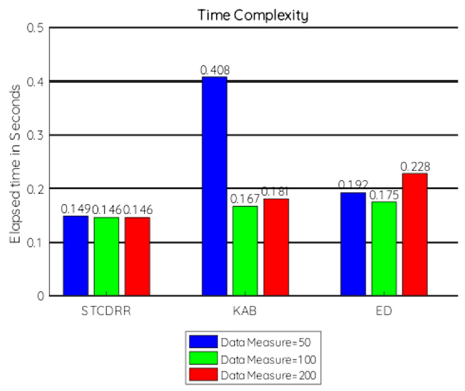
• This protocol outperforms in the context of the above parameters compared to the KAB (K-means algorithm based on the ANOVA model and Bartlett test) and ED (Euclidian distance) techniques.

The remainder of our paper is organized as follows: Section 2 presents the related works followed by Section 3 where background study is discussed in detail. Section 4 represents the methodologies, presumptions, and overall network representation then Section 5 represents the STCDRR (Spatial and Temporal Correlated Data Redundancy Reduction) protocol. Section 6 presents the experimental results and performance evaluation of the proposed STCDRR protocol followed by Section 7 which provides a detailed comparison of STCDRR protocol with two existing data aggregation techniques. Section 8 presents the conclusion and future work followed by the references.

2. Literature Review

An approach to eliminate the redundant spatial and temporal data was proposed in [7] which relies on two levels. The first level minimizes the data channeling using the Kalman filter for data approximation. The second level presents the elimination of redundant data based on grouping algorithms that work at the source level and the sink level separately. It provided a clear picture of data accuracy and reliability in terms of energy consumption. A novel data aggregation named REDA (Redundancy Elimination for Data Aggregation) in WSNs was proposed in [8]. It is based on a tree-based hierarchical clustered sensor network where energy savings are up to 40% regarding CH (cluster head) selection. It uses low bandwidth for the smooth functioning of the cluster head. The CHs are selected based on the lookup table formation generated by the residual energy and changing position of the CHs yield data transmission of the changed pattern.

Zhou et al. discussed an energy-structured data collection scheme that exploits the spatial and temporal correlation for the cluster-based sensor networks [9]. In the intra-cluster transmission dual prediction is used to deduce the redundancy temporally. A hybrid compact sensing method is used for inter-cluster data communication to reduce the data redundancy spatially. For the prediction model, an error threshold selection scheme is proposed which utilizes the combination between the energy dissipation and the recovery estimation making the proposed method fit for various sensor network applications. Tayea et al. proposed a data redundancy elimination approach that takes advantage of the spatial and temporal correlation among sensor observations to determine the sampling method for the distinct establishment of sensor nodes in the network area [10]. It eliminates the data emission rates by not violating the quality of the data. At the sink node, one back-end re-configuration algorithm is used which can reproduce the data to check the redundancy among the observed data set. A data aggregation based on a directional virtual backbone (DVBDAS) scheme is proposed by evaluating and balancing the energy load criteria as the virtual backbone which can build the clusters among the sensor nodes in the network [11]. The volume of energy dissipation is measured by calculating the optimized results of the cluster-based environment. Lu et al. proposed a data aggregation approach based on the distributed data convergence model exploiting the spatio-temporal correlation in WSNs [12]. This incorporates the centroid distance and similarity to estimate each cluster node’s attack degree. A data aggregation approach constructing an energy-efficient communication scheme is proposed in [13] by applying the GCC algorithm (Greedy Corrected Clustering) with the combination of the k-means algorithm to a LEACH (Low Energy Adaptive Clustering Hierarchy) protocol by exploiting the spatial correlation only. This algorithm limits the exploration of temporal data redundancy. This approach can reduce distortion, enhance the network lifetime and save energy.

In another work, Patil et al. presented a novel data redundancy reduction approach that is based on machine learning techniques [14]. It builds an aggregation tree of a defined number of sensor nodes. The Support Vector Machine (SVM) method eliminates the redundant data on the tree. Moreover, Locality Sensitive Hashing (LSH) eliminates the false data based on similarity and aggregates the non-redundant data to the superior node. Yuan et al. proposed a Correlation Degree based on Data Density (DDCD) clustering approach for calculating locally available data for the sink nodes in the network [15]. The sampled data is observed exploiting only the spatial correlation of the data to the sink node. No criteria have been mentioned for the temporal redundancy of the sampled data. It calculates the correlation among a sensor node’s data and its adjacent sensor node’s data enhancing the least contortion on their correlation. In [16], Redundancy Elimination for Accurate Data Aggregation (READA) is proposed where it eliminates the duplicate data by applying the grouping mechanism for organizing the total network into clusters where each cluster acts as cluster head. It is a delayed process where data loss and accuracy issues may occurs. Yousefi et al. suggest a structure-free real-time routing protocol for static sensor nodes in WSNs named RAG (Real-Time Data Aggregation) which exploits the temporal and spatial convergence of the data packets [17]. It takes advantage of available data by the waiting policy and aggregates the delayed data packets by the any-casting policy based on real-time data operating for the Medium Access Control (MAC) layer of the network. Some further modifications can be performed on the RAG protocol in order to be fit for mobile WSNs. Moreover, the spatial correlation-based data aggregation and enhancement for the smooth functioning of WSN applications can be implemented further.

3. Background Study

3.1. Spatial Correlation

Various applications of WSNs need dense deployment of sensor devices scattered in the sensor field. To satisfy the optimal coverage, the sensor nodes communicate with each other in the space domain. It results in the spatial correlation among the sensed data which are later processed and communicated in a huge number. The large volume of correlated data transmission increases the overall system overhead resulting in maximum energy utilization [18]. As the sensor nodes are characterized by battery-operated devices utilizing a finite source of energy it is important to exploit the spatial correlation among these data. Reducing the data redundancy by taking the advantage of spatial correlation the energy consumption can be decreased. Dense network topology results in multiple recordings of a single event which constitute the high correlation among sensor data. Inter-node and intra-node separation fluctuate the density of correlation [19].

3.2. Temporal Correlation

A wide range of applications of WSNs such as habitat monitoring, event tracking, defense, video surveillance requires sensor nodes to perform periodically. This sporadic assignment feature of sensor data transmission results in the collection of correlated data in multiple numbers of timestamps at a particular time [20]. The nature of the physical occurrence results in a temporal correlation between every successive consecutive monitoring of the sensor nodes. For adequate coverage of multiple sensor observations, the degree of correlation is dependent on the features of events that occurred [21].

3.3. Data Aggregation

The wireless sensor networks comprise tiny sources whose primary function is to detect various environmental phenomena and then forward them to the concerned base station. This communication carries a lot of cost, time, energy, accuracy, and reliability constraints [22]. Adopted by the finite source of energy the sensor node devices consume the maximum amount of energy, yielding a decreasing trend of battery life of devices. It may happen that any base station requires any information regarding any phenomenon happening near to it. Hence, in this scenario, there may be present any node to provide such spatio-temporal information related to it [23]. Temporal redundancy happens when there is a repeated phenomenon in various timestamps in a short time interval. Spatial redundancy happens when the phenomenon is correlated in space constraints, i.e., location based. Detection of the required event-based phenomenon which exhibits the spatial redundancy of the received data in the corresponding network fields [24]. They broadcast useful information in the direction of the desired sink after detecting the event. Remote sensor areas such as habitat monitoring, underwater sensor field are energy-consuming areas in the order of event detection and transmission. Repeated event detection phenomena often lead to network overhead in terms of energy, accuracy, latency, and reliability which eventually leads to redundant data transmission to sink [25]. Data aggregation can be chosen as an efficient solution to deal with the lacuna of energy for the sensor devices. This filtering technique can be levied both at the source and sink level to deal with the transmission of the redundant data. Aggregation functions such as MAX, MIN, SUM, COUNT [26] or any other mathematical calculations such as MATCH FUNCTION [27], CORRELATION COEFFICIENT TECHNIQUE [28] can be used to exploit the spatial and temporal data redundancy to achieve the desired goal [29].

4. Presumptions and Network Structuring

4.1. Presumptions

Let us consider S to be a multi-hop sensor network that consists of n sensor nodes and a solitary sink node. Let us consider the sensor network consists of cheap and small size sensors that have low power and memory. The nodes located in the network are invariable and kindred in nature. These nodes have distinctive d to discriminate them from other sensor nodes present in the network. The base station is provided with adequate hardware, ample memory, and abundant power. The source nodes are responsible for sensing different kinds of weather information such as voltage, light, humidity, temperature, etc. Here, sensing the data is performed by the source nodes. The aggregation task is completed by the aggregator nodes. The timing scheme is intermittent which means every source node at time slot j senses a new data measurement after time T node forms a vector of data measurement which is considered to be its weight function (wt).

4.2. Network Structuring

The network is of a hierarchical tree topology-based clustered structure. The nodes are considered to be static. The source nodes of the network can be either source (B) node or intermediate (C) node such as described in Equation (1).

$$C+B=n$$

(1)

Using the Tiny AGgregation protocol (TAG) [30], an aggregation tree is constructed with a base station as the tree root. TAG is a service of aggregation for the sensor networks. It provides an easy interface for data gathering based on the database query languages. It executes queries related to relevant aggregation in a time sequence manner. It executes in the network aggregation by combining the data flow processing and sending relevant readings by discarding irrelevant data readings [31]. The sink node provides the necessary queries to the network using the SPINS (Security Protocols for Sensor Networks) protocols [32]. SPINS is a type of security protocol consisting of the SPEN (Secure Network Encryption Protocol) [33] and the TESLA (a micro version of Timed, Efficient, Streaming, and Loss-tolerant Authentication Protocol) protocols. SPEN provides data confidentiality with the least overhead. TESLA broadcasts the authenticated data stream. SPINS building blocks authenticate the routing protocol [34].

4.3. State of the Art

Transmission of data between the cluster head and the members of the network is a type of single-hop communication. Periodically, the member nodes collect the data and send it to their appropriate cluster head. They have two phases that can diminish the redundant data induced by the nodes at each period. The sensor nodes sense the environment periodically to collect the data measures. Recently, the clustering method has emerged as an efficient technique to control topology due to its scalability and network maintenance nature. However, most of the existing techniques focus on the selection of the cluster head where the processing of the data is performed only at the cluster level, not at a particular node level. Here, we focus on the processing of the data both at the node level and the aggregator level. We have compared our proposed protocol STCDRR with two existing techniques, KAB and ED.

4.3.1. Data Aggregation at Source Level

The data collected by the sensor nodes in WSNs are highly correlated due to weather monitoring. It gives redundant data. If sensor nodes send all the collected data then energy wastage will lead to depletion of network lifetime. In WSNs, each period is divided into equal time slots. Periodic data collection forms a vector measure of the data. Suppose, in WSN $S,$ period $p$ is divided into time slots as [$a_1,a_2,\dots \dots a_r$] having vectors of measurements $N_i=\left[n_{i1},n_{i2},\dots \dots \dots .,n_{ir}\right]$. Suppose $S$ takes 4 measurements at the end of each period. It may happen that $N_i$ contains homogeneous measurements. So, the Similar function is assigned to identify whether two data measurements are similar or not. The Similar function for period $p$can be defined as:

$$\mathrm{Similar}(n_{ij}{n}_{ik})=\{\begin{array}{c}1 \mathrm{i}\mathrm{f} \Vert n_{ij}-n_{ik}\Vert \le \Psi \\ 0 \mathrm{e}\mathrm{l}\mathrm{s}\mathrm{e}\mathrm{w}\mathrm{i}\mathrm{s}\mathrm{e}\end{array}$$

where, $n_{ij,}{n}_{ik}$ are two similar measurements of a data vector and Ψ is the user-defined threshold value.

The weight of data $n_{ij}$is the number of similar measures of a vector. The source level aggregation searches for similar measurement of a data vector. In case it finds any redundant data, it deletes the same and updates the weight to 1.

4.3.2. Data Aggregation Using Similarity Function (JACCARD)

The JACCARD similarity Function supports many other similarity functions. So, it is widely used for various applications. It returns a value [0,1]. The higher the value, the more the similarity. In order to reduce the similar values, the highest cardinal value is treated as a duplicate pair and can be eliminated. The size of the data set is reduced before transmission to the sink node.

Example:

Suppose, there is a sensor $R$.

At a period $k$, calculated vector measurements $N_i=\left[7,7.8,7.9,9.2,9.5,9.6,9.7,10,10.1\right]$

Considering Ψ = 0.4,

The similarity function will transform the set of measures into $N_i^{\prime }=\left\{\left(7,3\right), \left(9,5\right), \left(10,2\right)\right\}$

where 3, 5, 2 are the weights of 7, 9, 10, respectively.

4.3.3. Data Aggregation Using the Variance Method (KAB)

Calculation of variance for the data set measurements is a way to find out the redundant data. The variance ($P$) can be identified between data measurements in a group of sets by applying the ANOVA model method. This method is used to detect data pair sets with similar values and can be eliminated.

For a threshold value £, the variance is calculated according to the Bartlett test and by applying the chi-square table.

When $P>\pounds ,$the data pair is considered to be redundant and can be eliminated.

If $P\le \pounds ,$ the data pair is valid and can be transmitted from the cluster head to the sink node.

The k-means algorithm is applied to the ANOVA model based on the calculated mean value of the data sets. Then, $n$ number of parent nodes is divided into $\sqrt{\frac{n}{2}}$ number of children nodes. At the end of each time period, one group of sets is selected from each data set along with their IDs for transmission.

4.3.4. Data Aggregation Using the Distance Function (ED)

A distance function is often used in WSNs for the deployment of sensor nodes in remote areas of a network. For data localization, the distance is estimated for the intra-sensor and inter-sensor nodes. The data measurement along with weights is calculated from the below formula:

$$D\left(X_i, X_j\right)=\sqrt{{\sum }_{k=1}^{\omega }\left(x_{ik}-x_{jk}\right)}²$$

where ω is the user-defined threshold value.

When, $D\le \omega$, the data set is considered redundant and can be eliminated before transmission [35].

5. STCDRR Protocol

The proposed STCDRR protocol enhances the reduction of data redundancy in WSNs. It operates in the source level and the aggregator level separately. First, it reduces the temporal data redundancy at the source level for a time T consists of small timestamps. Then it reduces the spatial data redundancy at the aggregator level using the Pearson Correlation Coefficient technique. The In-Network or Data aggregation method employs some aggregation functions which are SUM, COUNT, MAX, MIN, AVG to get a relevant aggregated result.

5.1. Eliminating Temporal Data Redundancy at Source Level

(I)

Assume that the root node observes the homogeneous (or identical) input estimate when the discerning neighborhood changes periodically or the time slot (j) is minimal. For reduction in dimensions, the juncture recognizes the identical data measurements.

(II)

These duplicate data are eliminated using the JACCARD similarity [36] match function.

The match function between two data measures is defined as

$$match(m_{ij},m_{jk})=\{\begin{array}{c}1 \mathrm{i}\mathrm{f} \Vert m_{ij}-m_{jk}\Vert \le \delta \\ 0, \mathrm{o}\mathrm{t}\mathrm{h}\mathrm{e}\mathrm{r}\mathrm{w}\mathrm{i}\mathrm{s}\mathrm{e}\end{array}$$

(2)

Equation (2), describes the mathematical formulation of the match function. Here, the threshold value is dependent on the type of application. The match function returns 1 for redundant data which means the two data values are similar.

(III)

The poundage of the input estimate is denoted by wt which is the numeral of the successive phenomenon of the identical or same measurement in the same set.

(IV)

After the accomplishment of the time interval, the root node converts the native vector of input estimates into a set accommodating the dissimilar input estimate as derived in Equation (3),

$$X_i=\{(x_{i1},w{t}_{i1}),\left(x_{i2},w{t}_{i2}\right),\dots , \left(x_{ik},w{t}_{ik}\right)\}$$

(3)

where k ≤ t.

(V)

The weighted cardinality of $X_i$ can be denoted as $\left|X_i\right|$ which is the grand total of all the input estimates in $X_i$which can be denoted as described in Equation (4).

$$wt\left(X_i\right)={{\displaystyle \sum }}_{j=1}^{\left|X_i\right|}wt\left(m_{ij}\right)=t$$

(4)

Algorithm 1 proposes the source level data redundancy reduction temporally using the JACCARD similarity index.

Algorithm 1: Data redundancy reduction using JACCARD

Input: new data measure$m_{ij}$,

Output: reduced dataset with unique values

Require: Existing data measurement value$M_i\left(m_{i1},m_{i2},\dots \dots ,m_{in}\right)$in time period$T$

Ensure: to forage homogeneous values in$M_i$

Start:

$for i=1:n$

$\{$

$for j=2:n+1$

$\{$

$p_i=\min \left(m\left(i,n\right),m\left(j,n\right)\right)$

$q_i=\max \left(m\left(i,n\right),m\left(j,n\right)\right)$

$\}$

$ratio=\frac{{{\displaystyle \sum }}_{i=1}^n{p}_i}{{{\displaystyle \sum }}_{j=1}^n{q}_j}$

$if\left(ratio<\delta \right)$

$data m_{in} forwarded to sink$

$\}$

Stop

After the time period T, the source node aggregates the non-redundant data measurement to the sink node rather than aggregating the original data vector.

5.2. Eliminating Spatial Data Redundancy at Aggregator Level

The intermediate nodes are responsible for executing the aggregation function at the aggregator level. The root nodes dispatch the aggregated input value set to the aggregator nodes after data collection. Corresponding the child node distributes the set of measured data vectors along with their weights to each aggregator node. To eliminate the data redundancy among the collected data set implementation of the correlation coefficient technique method is a suitable solution. In this paper, we have used Pearson’s Correlation Coefficient method to discover the highly correlated input set [37]. Thus, discarding the unwanted similar data set, only the relevant non-redundant data sets are forwarded to the sink node. A lesser number of transmissions can effectively reduce the overall energy consumption enhancing the network lifetime.

An overview of Pearson’s Correlation Coefficient ($\rho$) method.

(1)

This technique is a covariance measurement of the correlation degree between two input set estimates. Sensor data sets associated with their weights can be evaluated using this technique. Its value varies from −1 to 1. A negative correlation exists when the data set results in the value of −1. Getting a resulting value of 0 means there is no correlation. The positive correlation is derived when a value of 1 is obtained among two input sets.

(2)

We can formulate this correlation function for two sensor input sets and along with their weights as follows:

$$\rho X_i,Y_j=\frac{cov\left(X_i,Y_j;wt\right)}{\surd cov\left(X_i,X_i;wt\right)cov\left(Y_j,Y_j;wt\right)}$$

(5)

$$cov\left(X_i,Y_j;wt\right)=\frac{{\sum }_{i=1}^{n}w{t}_i\left(X_i-m\left(X_i;wt\right)\right)\left(Y_j-m\left(Y_j;wt\right)\right)}{{\sum }_{i=1}^{n}w{t}_i}$$

(6)

$$m\left(X_i;wt\right)=\frac{{\sum }_{i=1}^{n}w{t}_i{X}_i}{{\sum }_{i=1}^{n}w{t}_i}$$

(7)

where,

• $cov\left(X_i,Y_j;wt\right)=$ The weighted covariance between $X_i$ and $Y_j$,
• n = Gross number of input estimates in every data set,
• $m\left(X_i;wt\right)=$ The weighted mean of $X_i$,
• $m\left(Y_j;wt\right)=$ The weighted mean of $Y_j$.

Equations (5)–(7) describe the mathematical formulation of the Pearson Correlation Coefficient and Covariance and Weighted Mean of two sets, respectively.

(3)

Here $“\tau ”$ is the threshold value that is decided by the type of application. Two input measures are highly correlated if and only if it satisfies Equation (8) as follows:

$${\rho }_{X_i{Y}_j}<\tau$$

(8)

(4)

The agglomerated value is derived for every single pair of received data sets. The correlation coefficient value less than the threshold value indicates redundancy among the two data sets and repudiates such pairs containing either one or two sets.

(5)

Then, it computes the new weight value among the two compared input sets. Then the aggregator picks the one which has the highest cardinality among the two. Then the new aggregated value along with its latest weight is added to the record.

Algorithm 2 is designed for the aggregator level aggregation using the Pearson’s Correlation Coefficient method. After receiving the aggregated value of the non-redundant data set, the aggregated input value should be transmitted to the base station.

Algorithm 2: Pearson’s Correlation Coefficient

Input: Data measure set$X_i , Y_j$

Output: Aggregated data set along with weigh with highest cardinality

Require: set of input measures$X=\left\{X_1,X_2,X_3,\dots \dots \dots \dots ,X_x\right\}$,$\tau$(threshold value)

Ensure: vector of selected input set Q

initialize Q, $R_1$, H = {$\varnothing$}

Start:

forevery input set$X_i\in X$do

$R_1=R_1 \cup \left\{X_i\right\}$

end for

$H=H \cup \left\{R_1\right\}$

rerun

for respective pairs of input sets ($X_i,Y_j$) $\in R_1$ do

if ${\rho }_{X_i,Y_j}<\tau$then

consider $\left|X_i\right|\ge \left|Y_j\right|$

discard each set of input sets which include either $X_i$or $Y_j$ from H

$wt\left(X_i\right)$= number of dropped pairs incremented to 1

Q = Q $\cup \left\{X_i,wt\left(X_i\right)\right\}$

else

H = H $\cup \left\{X_i\right\} \cup \left\{Y_J\right\}$

end if

end for

tillnone of the set$X_i$in H

return Q

Stop

6. Performance Evaluation

For experimental results, we have taken the Intel Berkley Research lab data set where 46 Mica2Dot sensors collected the different weather information which was light, humidity, voltage, temperature, pressure, along with the date and timestamp, using a 31 s interval [38]. This real data set also contains epoch and moteid. Here, the data are collected on the TinyOs [39] operating system platform using the TinyDB [40] query processing and in-network aggregation procedure. In our experiment, we have taken the temperature attribute for ease of work. We evaluated the experiment on nearly 2.5 million data readings collected from the sensors. Here, we assumed that a recurrent cluster head is situated at the center place of the laboratory and collects the data from each sensor placed inside. At first, every node reads the collected data measurement periodically and sends its data set along with its weights at the end of the step. By comparing these steps in three different algorithms, an observation can be made to check the efficiency with respect to the two other existing approaches. The implementation part is performed in the MATLAB simulator [41]. In our work, we have compared our proposed protocol STCDRR with two algorithms which are namely KAB (K-means algorithm based on the ANOVA model and Bartlett test) and ED (Euclidian distance) [42]. ED is a simple and effective technique used in various applications [43,44,45,46,47,48]. We have the comparison results in terms of the key parameters and performance metrics which are described in Section 6.1 and 6.2.

6.1. Key Parameters

The important parameters those can be associated with the underlined work are as follows.

6.1.1. Threshold Function Value

This is the threshold value that is user-defined. As our protocol STCDRR works in two levels namely the source level and the sink level. Match function threshold value is taken for the source level data aggregation where we have used the JACCARD similarity match function to reduce the temporal data redundancy. Correlation Coefficient threshold value is taken for the sink level data aggregation where we have used the Pearson’s Correlation Coefficient technique to reduce the spatial data redundancy.

6.1.2. Data Measures $\left(\mathsf{\alpha }\right)$

The number of data measures recorded in the timestamp “T” can give the comparative result of our proposed protocol STCDRR with KAB and ED.

6.2. Performance Metrics

The performance metrics for our work are as follows.

Aggregation Ratio

The aggregation ratio can be defined as the total number of data packets generated to the total number of data measurements sent. Each sensor node finds the similarity between the data measurements collected for each time period during the local aggregation process. The data measurements are assigned with a weight dependent on the threshold value chosen for the experiment. With the increase or decrease of the threshold the data redundancy among data increases or decreases, respectively, after applying the similarity match function during the local aggregation process. The poundage of the input estimate is given in

Table 1. Parameters table.

Sl.No.	Parameter	Notation	Value
1	No. of Data Measurements	$\alpha$	50, 100, 200
2	Threshold of Distance Function	$t_d$	0.3, 0.4, 0.5, 0.7
3	Threshold of Correlation Coefficient	$\tau$	0.3, 0.4, 0.45, 0.5
4	Threshold of Match Function	$\delta$	0.02, 0.04, 0.06, 0.1

as numerical values.

Energy Consumption

It is defined as total energy spent for executing the process of data packets consequently in the network. As the data aggregation is divided into two phases, namely data aggregation at source level and data aggregation at sink level so energy spent on these levels need to be calculated and reduced for an enhanced network lifetime.

Data Accuracy

Data accuracy is the representation of data loss measurement. It can be obtained by dividing the total number of data packets measured by the sensor nodes which are similar in nature and do not get forwarded to sink over the whole data measure taken by the sensor for a particular time period, after applying the local data aggregation. Evaluation of data accuracy is based on the percentage of data loss measures collected at the cluster head.

Time Complexity

The accuracy of an efficient algorithm is based on the measurement of the time taken to execute the whole process. The execution time on an algorithm is dependent on the threshold value taken for the experiment.

7. Experimental Results

Considering the above performance measures and key parameters we have calculated and compared our proposed protocol STCDRR with two existing algorithms, KAB and ED in terms of energy consumption, aggregation ratio, data accuracy, and time complexity. Experimental results show that the STCDRR protocol performs well against to KAB and ED and reduces the energy consumption carried out for forwarding data packets from the source level to the destination level in the network resulting in an enhanced network lifetime. Table 1 summarizes the key parameters taken for our experiment.

(1)

The number of sensors calculated by individual sensor node for a period has some values. Here we have taken 3 values 50, 100, 200. It is denoted by α.

(2)

The threshold value for the distance function is denoted by $t_d$. We have taken 4 different values 0.3, 0.4, 0.5, 0.7 to check the difference in results for each value.

(3)

To compare at the aggregator level the threshold values are taken to be 0.3, 0.4, 0.45, 0.5.

(4)

The thresholds for the match function are 0.02, 0.04, 0.06, 0.1.

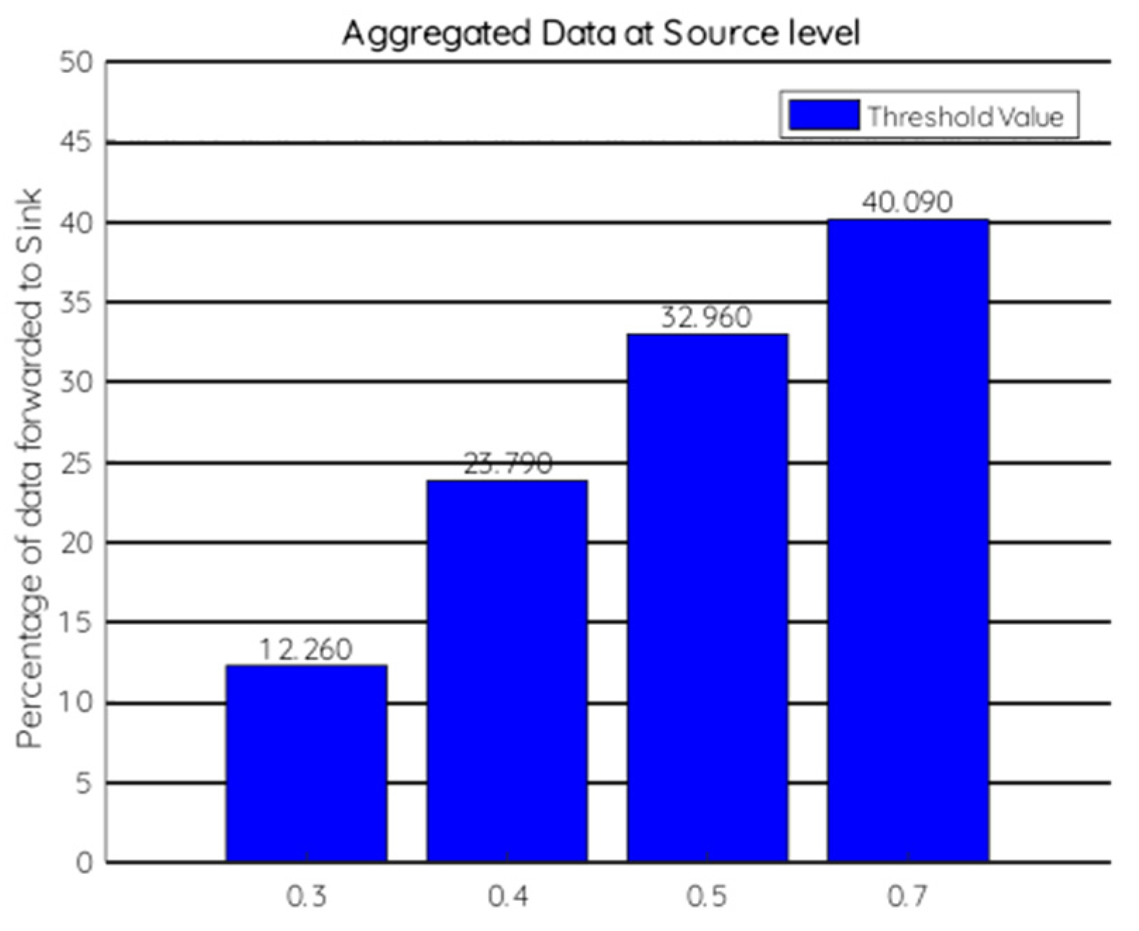
7.1. Source Level Experiment

Aggregated data after source level aggregation is forwarded to the sink. From Figure 1, we can observe that the percentage of the aggregated data is on an increasing trend with respect to the increase in the threshold value.

7.2. Sink Level Experiment

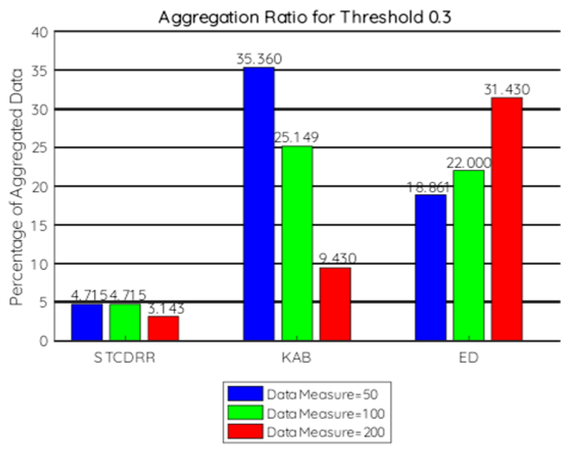
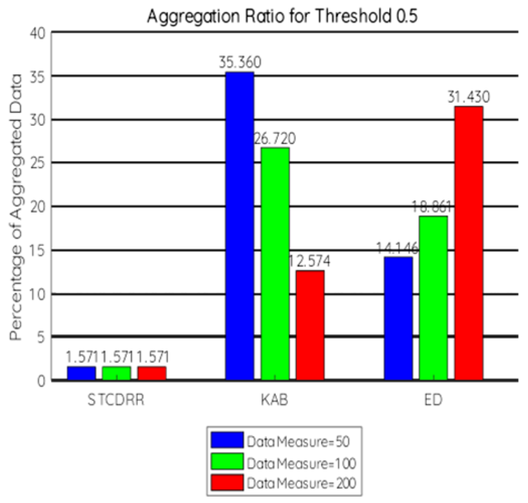
7.2.1. Aggregation Ratio

Figure 2, Figure 3 and Figure 4 shows the remaining aggregated data in percentage after applying the sink level aggregation process. These aggregated data are forwarded to the cluster head after filtering. One hundred percent of the data will be forwarded to the sink if the aggregation process is not being applied. However, it is observed in the figures below that the percentage of aggregated data is subsequently low in our proposed technique as compared to the other two techniques. After each period, the sensor node sends data to the cluster head. It is noticeable that after applying the aggregation process data collection by the sensor node is reduced by 75% up to 93%. Hence, it is concluded that the STCDRR protocol is efficient in terms of aggregation ratio by eliminating the redundant data measurements after completion of each time period as compared to KAB and ED.

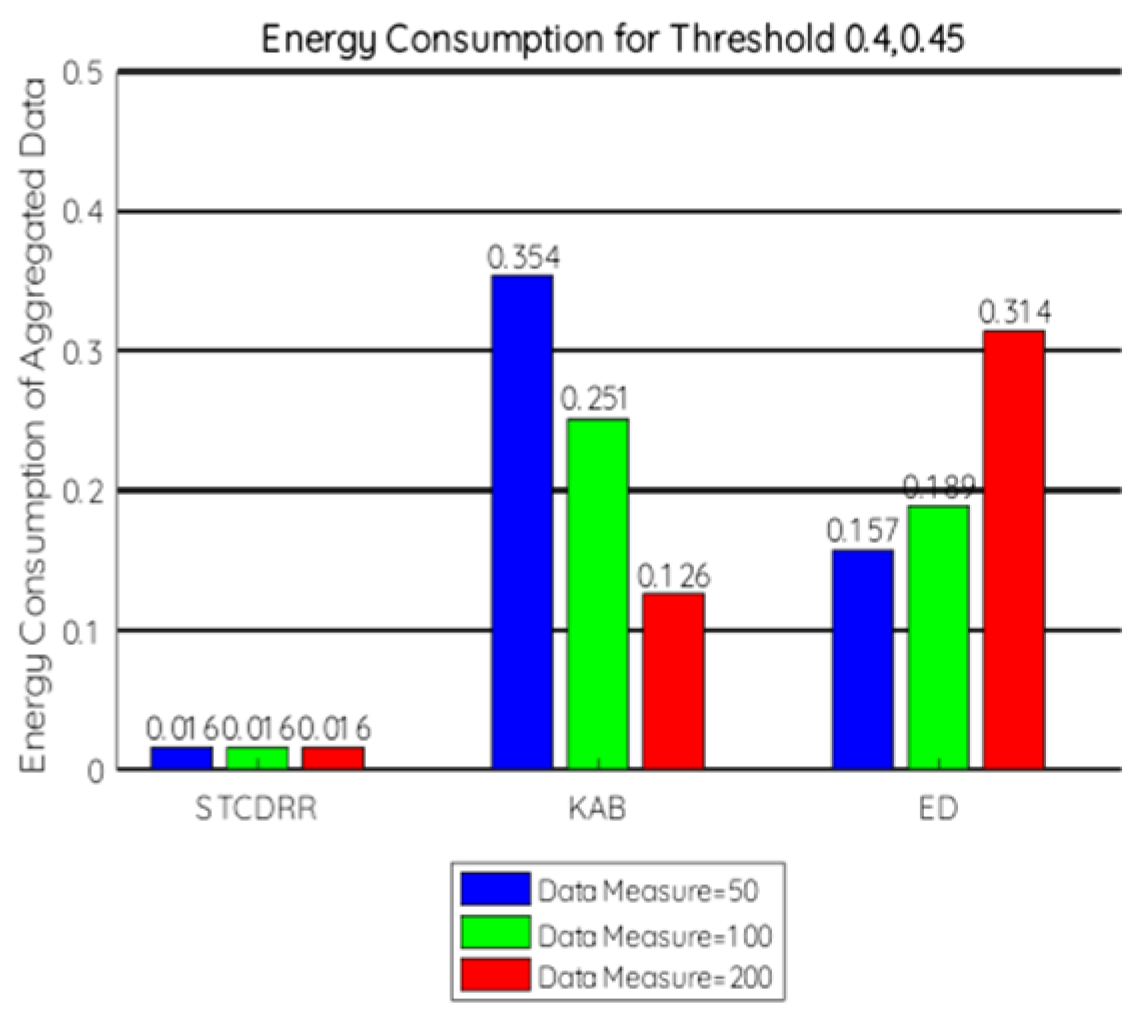
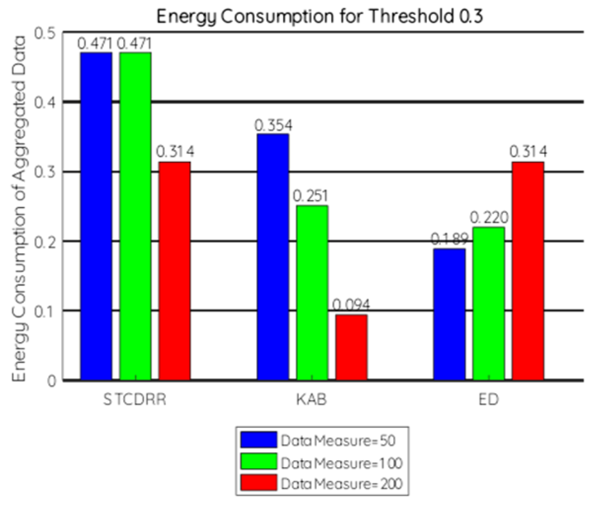
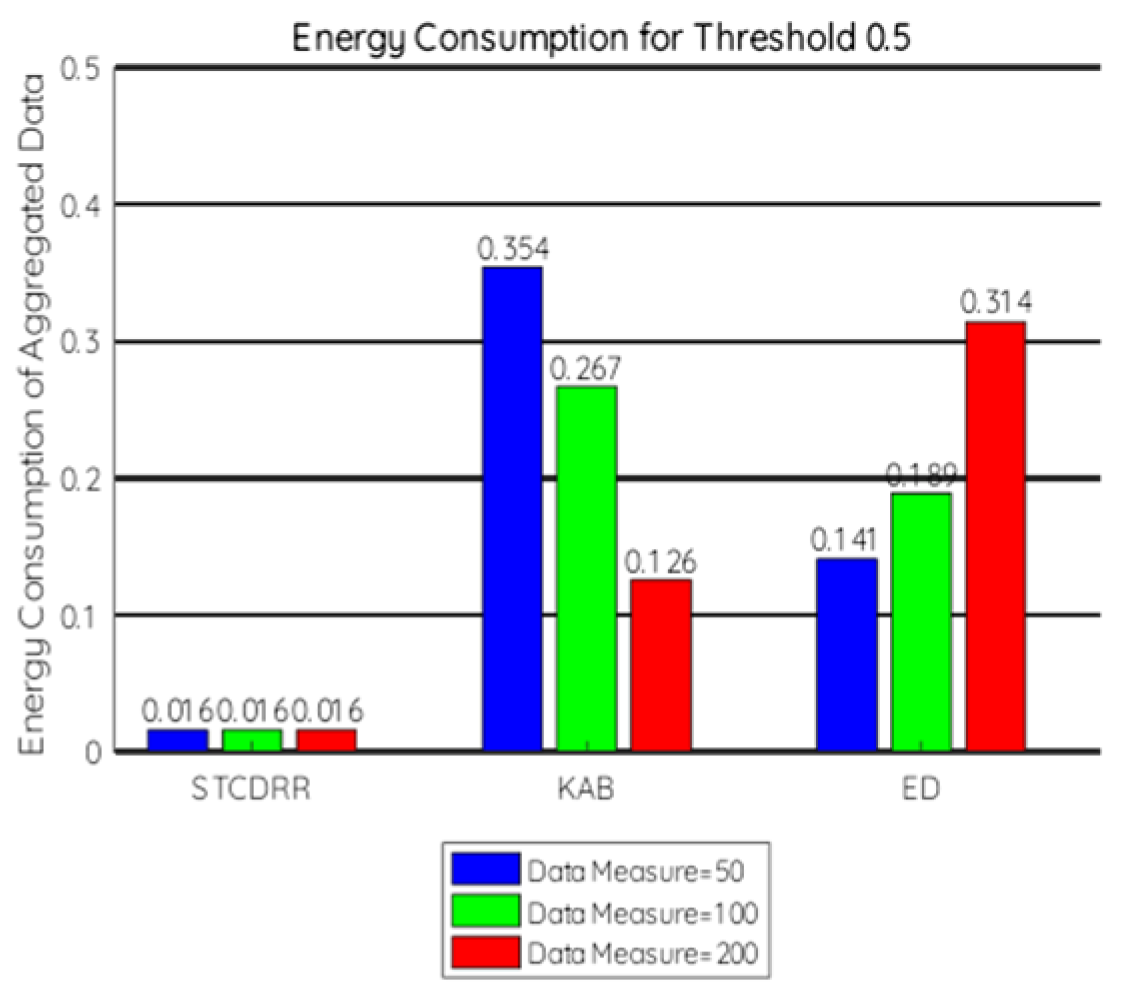
7.2.2. Energy Consumption

Energy consumption for varying threshold values can be observed in Figure 5, Figure 6 and Figure 7. It is observed that with a minimum threshold value, i.e., 0.3 the energy consumption of our proposed approach is comparatively higher than KAB and ED. However, with the increase of the threshold value, there is a subsequent decrease in energy consumption in the proposed approach which implies the efficiency of the proposed algorithm. The STCDRR protocol can save from 70% up to 90% of the energy of the sensor node which makes it suitable for enhancing the network lifetime. Here, we have calculated the energy in terms of miliJoule (mJ).

Calculation of Energy Consumption:

$$E=P\times \left(\frac{t}{1000}\right)$$

(9)

where,

• $E$ = Energy measured in miliJoules (mJ) or in Kilowatt-hours (Kwh),
• $P$ = Power units in Watts,
• $t$ = Time over which the power or energy was consumed.

Example:

Let us consider 6300 rows of temperature attributes of the data set.

Suppose, the average voltage of 6300 rows = 2.6

Calculating the voltage for 6300 rows of data = 6300 $\times$ 2.6 = 16,380 which is 1.571 percentage of aggregated data.

So, calculation of energy consumption will be,

E = 6300 $\times$ 0.01571 = 98.97 (99) which is the number of aggregated data to the cluster head.

So, the calculation of total energy consumption will be:

1 node consumes 2.6 mJ energy AD 99 nodes will consume 99 $\times$ 2.6 = 257.33 mJ of V.

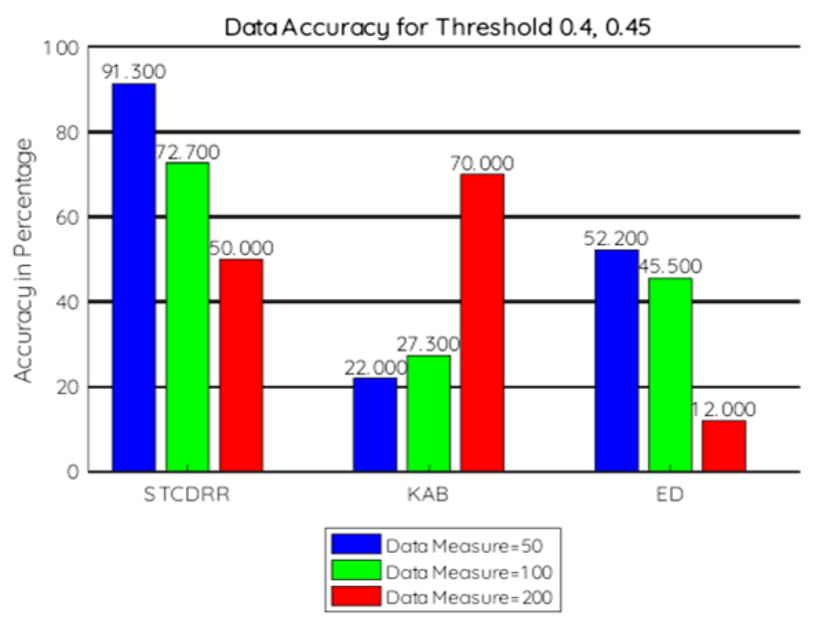
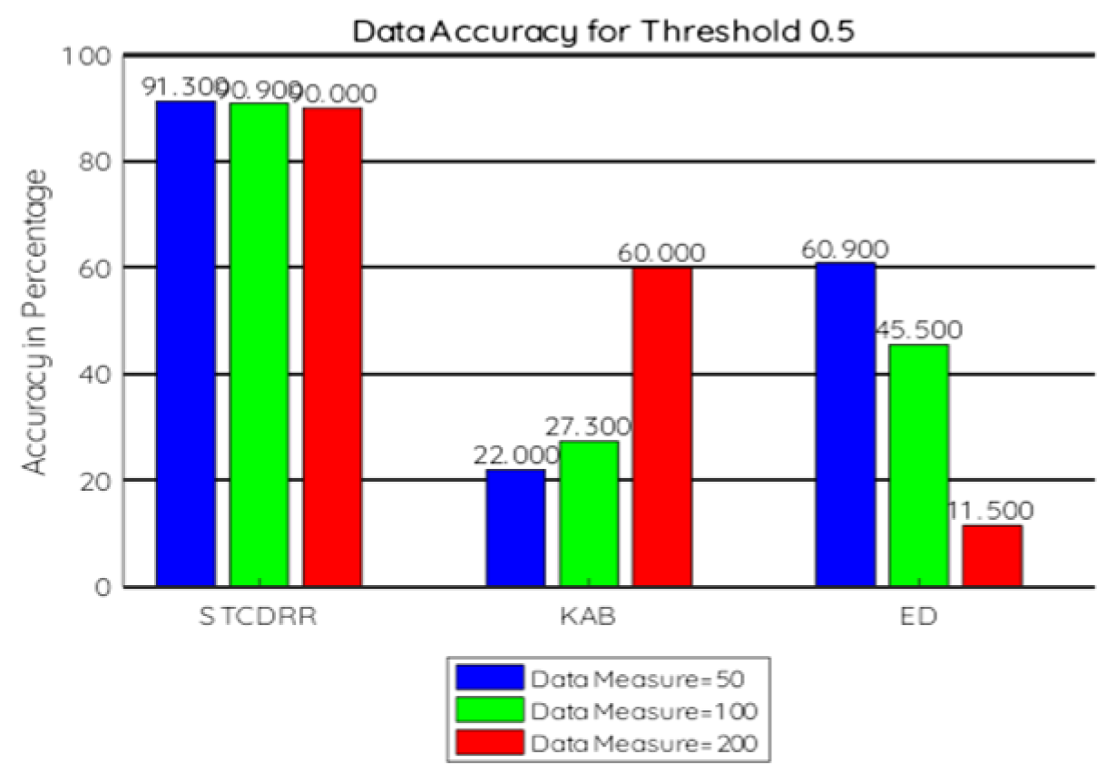
7.2.3. Data Accuracy

The main goal is to send very less data to the destination node or sink. In the KAB technique, only one set of data elements is sent among a group of sets to the sink which in turn increases the loss of data measurements. However, in ED, the integrity of conservation of information is maintained. Figure 8, Figure 9 and Figure 10 imply the data accuracy for three approaches with varying threshold values. It is clearly visible from the graph that the proposed protocol gives the best results in terms of measurement of the accuracy of the data.

7.2.4. Time Complexity

The execution time required for a process is the total time taken for the completion of the task. In KAB, the execution time is calculated on the basis of the number of iterations of the loops in the algorithm. In ED, the comparison between two redundant sets takes less computation time as compared to KAB. In our proposed approach the execution time taken to identify the redundant set is least as compared to KAB and ED as it uses the JACCARD Similarity Function. Complexity in computation is $O\left(\left|X_i\right|²\right)$ which is almost half of the data measure sensed at each period eventually reducing the energy consumption. Time complexity in KAB is in order of $O\left(x\right)$ where $x$ is the number of total received data sets. In, ED complexity is, at most, in order $O\left(x²\right)$.

This comparison is analyzed in Figure 11.

7.2.5. Discussion

ED preserves the data integration as compared to KAB and STCDRR as the distance function has the highest cardinality as compared to the other two methods. Data loss measurement is good in KAB as compared to that in ED and STCDRR as it constitutes the ANOVA model irrespective of the increase or decrease of distance and vice-versa. Data accuracy and time complexity in STCDRR are high as compared to KAB and ED. Data latency at the cluster head is high for the STCDRR protocol as it undergoes approximately 30 more rounds of execution as compared to KAB and ED. For energy efficiency, the STCDRR protocol can be chosen as an efficient protocol as it preserves up to 90% of total energy.

8. Conclusions and Future Work

In Wireless Sensor Networks, eliminating the duplicate data measurements is a very limiting task to transmitting the required information as it absorbs most of the battery-driven energy. So, it is very important to conserve the finite amount of energy to enhance the overall network lifetime. In order to increase the network lifetime, it is necessary to reduce the data redundancy to eliminate the duplicate data. In this work, we have proposed the STCDRR protocol which works in two levels namely the source level and the sink level. Data aggregation is carried out by utilizing the JACCARD similarity function in the source level and Pearson’s Correlation Coefficient technique in the sink level or aggregator. Our approach uses a real data set and it is implemented in the MATLAB simulator for data accuracy, energy consumption, and aggregation ratio. The graphical results show our protocol outperforms the existing techniques, KAB and ED. For future work, we will utilize this protocol for a multi-attribute data set with a greater number of key parameters and performance measures to minimize energy utilization for an enhanced network lifetime.

In this work, we have used only one data set and only one attribute (temperature) of the data set. It is a limitation of this work. The potential result that our proposed protocol will give for two datas ets or two attributes of one data set is yet to be explored. In the future, we will try to experiment with our protocol, STCDRR, using more than one data set.

References

1. Lazarescu, M.T. Design of a WSN platform for long-term environmental monitoring for IoT applications. IEEE J. Emerg. Sel. Top. Circuits Syst. 2013, 3, 45–54. [Google Scholar] [CrossRef] [Green Version]
2. Chi, Q.; Yan, H.; Zhang, C.; Pang, Z.; Xu, L.D. A reconfigurable smart sensor interface for industrial WSN in IoT environment. IEEE Trans. Ind. Inf. 2014, 10, 1417–1425. [Google Scholar]
3. Akyildiz, I.F.; Su, W.; Sankarasubramaniam, Y.; Cayirc, E. Wireless sensor networks: A survey. Comput. Netw. 2002, 38, 393–422. [Google Scholar] [CrossRef] [Green Version]
4. Villas, L.A.; Boukerche, A.; de Oliveira, H.A.; de Araujo, R.B.; Loureiro, A.A. A spatial correlation aware algorithm to perform efficient data collection in wireless sensor networks. Ad Hoc Netw. 2014, 12, 69–85. [Google Scholar] [CrossRef]
5. Varun, M.C.; Akan, O.B.; Akyildiz, I.F. Spatio-temporal correlation: Theory and applications for wireless sensor networks. Comput. Netw. 2004, 45, 245–259. [Google Scholar]
6. Maivizhi, R.; Yogesh, P. Spatial correlation based data redundancy elimination for data aggregation in wireless sensor networks. In Proceedings of the 2020 International Conference on Innovative Trends in Information Technology (ICITIIT), Kottayam, India, 13–14 February 2020; IEEE: Piscataway, NJ, USA, 2020; pp. 1–5. [Google Scholar]
7. Yemeni, Z.; Wang, H.; Ismael, W.M.; Wang, Y.; Chen, Z. Reliable spatial and temporal data redundancy reduction approach for WSN. Comput. Netw. 2021, 185, 107701. [Google Scholar] [CrossRef]
8. Yadav, S.; Yadav, R.S. Redundancy elimination during data aggregation in wireless sensor networks for IoT systems. In Recent Trends in Communication, Computing, and Electronics; Springer: Singapore, 2019; pp. 195–205. [Google Scholar]
9. Zhou, Y.; Yang, L.; Yang, L.; Ni, M. Novel energy-efficient data gathering scheme exploiting spatial-temporal correlation for wireless sensor networks. Wirel. Commun. Mob. Comput. 2019, 2019, 4182563. [Google Scholar] [CrossRef]
10. Tayeh, G.B.; Makhoul, A.; Perera, C.; Demerjian, J. A spatial-temporal correlation approach for data reduction in cluster-based sensor networks. IEEE Access 2019, 7, 50669–50680. [Google Scholar] [CrossRef]
11. Zhang, J.; Liu, S.; Tsai, P.W.; Zou, F.; Ji, X. Directional virtual backbone based data aggregation scheme for Wireless Visual Sensor Networks. PLoS ONE 2018, 13, e0196705. [Google Scholar] [CrossRef]
12. Lu, Y.; Sun, N. A resilient data aggregation method based on spatio-temporal correlation for wireless sensor networks. Eur. J. Wirel. Commun. Netw. 2018, 1, 157. [Google Scholar] [CrossRef] [Green Version]
13. Li, Y.; Zheng, X.; Liu, J.; Hu, N.; Yang, G. Application of energy-efficient data gathering to wireless sensor network by exploiting spatial correlation. Sens. Mater. 2018, 30, 577–585. [Google Scholar] [CrossRef]
14. Patil, P.; Kulkarni, U. SVM based data redundancy elimination for data aggregation in wireless sensor networks. In Proceedings of the 2013 International Conference on Advances in Computing, Communications and Informatics (ICACCI), New York, NY, USA, 22–25 August 2013; IEEE: Piscataway, NJ, USA, 2013; pp. 1309–1316. [Google Scholar]
15. Yuan, F.; Zhan, Y.; Wang, Y. Data density correlation degree clustering method for data aggregation in WSN. IEEE Sens. J. 2013, 14, 1089–1098. [Google Scholar] [CrossRef]
16. Khedo, K.; Doomun, R.; Aucharuz, S. READA: Redundancy elimination for accurate data aggregation in wireless sensor networks. Wirel. Sens. Netw. 2010, 2, 300. [Google Scholar] [CrossRef] [Green Version]
17. Yousefi, H.; Yeganeh, M.H.; Alinaghipour, N. Structure-free real-time data aggregation in wireless sensor networks. Comput. Commun. 2012, 35, 1132–1140. [Google Scholar] [CrossRef]
18. Misra, Sudip, and Subarna Chatterjee. Social choice considerations in cloud-assisted WBAN architecture for post-disaster healthcare: Data aggregation and channelization. Inf. Sci. 2014, 284, 95–117. [Google Scholar] [CrossRef]
19. Curiac, D.I.; Volosencu, C.; Pescar, D.; Jurca, L. Redundancy and its applications in wireless sensor networks: A survey. WSEAS Trans. Comput. 2009, 8, 705–714. [Google Scholar]
20. Pielli, C.; Zucchetto, D.; Zanella, A. An interference-aware channel access strategy for WSNs exploiting temporal correlation. IEEE Trans. Commun. 2019, 67, 8585–8597. [Google Scholar] [CrossRef]
21. Buckler, M.; Bedoukian, P.; Jayasuriya, S. EVA2: Exploiting temporal redundancy in live computer vision. In Proceedings of the 2018 ACM/IEEE 45th Annual International Symposium on Computer Architecture (ISCA), Los Angeles, CA, USA, 1–6 June 2018; IEEE: Piscataway, NJ, USA, 2018. [Google Scholar]
22. Xu, X.; Ansari, R.; Khokhar, A.; Vasilakos, A.V. Hierarchical data aggregation using compressive sensing (HDACS) in WSNs. ACM Trans. Sens. Netw. 2015, 11, 1–25. [Google Scholar] [CrossRef]
23. Sengupta, A.; Kachave, D. Spatial and temporal redundancy for transient fault-tolerant datapath. IEEE Trans. Aerosp. Electron. Syst. 2017, 54, 1168–1183. [Google Scholar] [CrossRef]
24. Neha, B.; Panda, S.K.; Sahu, K.P.; Sahoo, K.S.; Gandomi, A.H. A Systematic Review on Osmotic Computing. ACM Trans. Internet Things 2022, 3, 1–30. [Google Scholar] [CrossRef]
25. Verma, N.; Singh, D. Data redundancy implications in wireless sensor networks. Procedia Comput. Sci. 2018, 132, 1210–1217. [Google Scholar] [CrossRef]
26. Zhang, P.; Wang, J.; Guo, K.; Wu, F.; Min, G. Multi-functional secure data aggregation schemes for WSNs. Ad Hoc Netw. 2018, 69, 86–99. [Google Scholar] [CrossRef]
27. Alzaid, H.; Foo, E.; Nieto, J.G. RSDA: Reputation-based secure data aggregation in wireless sensor networks. In Proceedings of the Ninth International Conference on Parallel and Distributed Computing, Applications and Technologies, Dunedin, New Zealand, 1–4 December 2008; IEEE: Piscataway, NJ, USA, 2008. [Google Scholar]
28. Ghosh, S.; De, S.; Chatterjee, S.; Portmann, M. Learning-based adaptive sensor selection framework for multi-sensing WSN. IEEE Sensors Journal 2021, 21, 13551–13563. [Google Scholar] [CrossRef]
29. Jesus, P.; Baquero, C.; Almeida, P.S. A survey of distributed data aggregation algorithms. IEEE Commun. Surv. Tutor. 2014, 17, 381–404. [Google Scholar] [CrossRef] [Green Version]
30. Madden, S.; Franklin, M.J.; Hellerstein, J.M. TAG: A tiny aggregation service for ad-hoc sensor networks. ACM Sigops Oper. Syst. Rev. 2002, 36, 131–146. [Google Scholar] [CrossRef]
31. Ujawe, P.V.; Khiani, S. Review on data aggregation techniques for energy efficiency in wireless sensor networks. Int. J. Emerg. Technol. Adv. Eng. 2014, 4, 7. [Google Scholar]
32. Perrig, A.; Szewczyk, R.; Tygar, J.D.; Wen, V.; Culler, D.E. SPINS: Security protocols for sensor networks. Wirel. Netw. 2002, 8, 521–534. [Google Scholar] [CrossRef]
33. Tobarra, L.; Cazorla, D.; Cuartero, F. Formal analysis of sensor network encryption protocol (snep). In Proceedings of the 2007 IEEE International Conference on Mobile Adhoc and Sensor Systems, Pisa, Italy, 8–11 October 2007; IEEE: Piscataway, NJ, USA, 2007. [Google Scholar]
34. Li, X.; Ruan, N.; Wu, F.; Li, J.; Li, M. Efficient and enhanced broadcast authentication protocols based on multilevel μTESLA. In Proceedings of the 2014 IEEE 33rd International Performance Computing and Communications Conference (IPCCC), Austin, TX, USA, 5–7 December 2014; IEEE: Piscataway, NJ, USA, 2014. [Google Scholar]
35. Harb, H.; Abdallah, M.; Couturier, R. An enhanced K-means and ANOVA-based clustering approach for similarity aggregation in underwater wireless sensor networks. IEEE Sens. J. 2015, 15, 5483–5493. [Google Scholar] [CrossRef] [Green Version]
36. Bag, S.; Kumar, S.K.; Tiwari, M.K. An efficient recommendation generation using relevant Jaccard similarity. Inf. Sci. 2019, 483, 53–64. [Google Scholar] [CrossRef]
37. Zhou, H.; Deng, Z.; Xia, Y.; Fu, M. A new sampling method in particle filter based on Pearson correlation coefficient. Neurocomputing 2016, 216, 208–215. [Google Scholar] [CrossRef]
38. Madden, S. Intel Berkeley Research Lab. 2004. Available online: http://db.csail.mit.edu/labdata/labdata.html (accessed on 15 August 2021).
39. Amjad, M.; Sharif, M.; Afzal, M.K.; Kim, S.W. TinyOS-new trends, comparative views, and supported sensing applications: A review. IEEE Sens. J. 2016, 16, 2865–2889. [Google Scholar] [CrossRef]
40. Kim, D.O.; Liu, L.; Shin, I.S.; KimKim, J.J. Spatial TinyDB: A spatial sensor database system for the USN environment. Int. J. Distrib. Sens. Netw. 2013, 9, 512368. [Google Scholar] [CrossRef]
41. Mikkili, S.; Panda, A.K.; Prattipati, J. Review of real-time simulator and the steps involved for implementation of a model from MATLAB/SIMULINK to real-time. J. Inst. Eng. Ser. B 2015, 96, 179–196. [Google Scholar] [CrossRef]
42. Harb, H.; Makhoul, A.; Tawbi, S.; Couturier, R. Comparison of different data aggregation techniques in distributed sensor networks. IEEE Access J. 2017, 5, 4250–4263. [Google Scholar] [CrossRef]
43. Rout, S.; Sahoo, K.S.; Patra, S.S.; Sahoo, B.; Puthal, D. Energy Efficiency in Software Defined Networking: A Survey. SN Comput. Sci. 2021, 2, 308. [Google Scholar] [CrossRef]
44. Panda, B.S.; Bhatta, B.K.; Mishra, S.K. Improved energy-efficient target coverage in wireless sensor networks. In Proceedings of the International Conference on Computational Science and Its Applications, Trieste, Italy, 3–6 July 2017; Springer: Cham, Switzerland, 2017; pp. 350–362. [Google Scholar]
45. Nayak, R.P.; Sethi, S.; Bhoi, S.K.; Sahoo, K.S.; Jhanjhi, N.; Tabbakh, T.A.; Almusaylim, Z.A. TBDDoSA-MD: Trust-Based DDoS Misbehave Detection Approach in Software-defined Vehicular Network (SDVN). Comput. Mater. Contin. 2021, 69, 3513–3529. [Google Scholar] [CrossRef]
46. Pande, S.K.; Panda, S.K.; Das, S.; Sahoo, K.S.; Luhach, A.K.; Jhanjhi, N.Z.; Alroobaea, R.; Sivanesan, S. A resource management algorithm for virtual machine migration in vehicular cloud computing. Comput. Mater. Contin. 2021, 67, 2647–2663. [Google Scholar] [CrossRef]
47. Mishra, S.K.; Mishra, S.; Alsayat, A.; Jhanjhi, N.Z.; Humayun, M.; Sahoo, K.S.; Luhach, A.K. Energy-aware task allocation for multi-cloud networks. IEEE Access 2020, 8, 178825–178834. [Google Scholar] [CrossRef]
48. Maity, P.; Saxena, S.; Srivastava, S.; Sahoo, K.S.; Pradhan, A.K.; Kumar, N. An Effective Probabilistic Technique for DDoS Detection in OpenFlow Controller. IEEE Syst. J. 2021, 1–10. [Google Scholar] [CrossRef]
Figure 1. Percentage of data after applying source level aggregation.
Electronics 11 00989 g001
Figure 2. Aggregation ratio for threshold, 0.3.
Electronics 11 00989 g002
Figure 3. Aggregation ratio for thresholds, 0.4, 0.45.
Electronics 11 00989 g003
Figure 4. Aggregation ratio for threshold, 0.5.
Electronics 11 00989 g004
Figure 5. Energy consumption in mJ for threshold, 0.3.
Electronics 11 00989 g005
Figure 6. Energy consumption in mJ for thresholds, 0.4, 0.45.
Electronics 11 00989 g006
Figure 7. Energy consumption in mJ for threshold, 0.5.
Electronics 11 00989 g007
Figure 8. Data accuracy for threshold, 0.3.
Electronics 11 00989 g008
Figure 9. Data accuracy for thresholds, 0.4, 0.45.
Electronics 11 00989 g009
Figure 10. Data accuracy for threshold, 0.5.
Electronics 11 00989 g010
Figure 11. Execution time of STCDRR, KAB, ED in seconds for data measurements 50, 100, and 200.
Electronics 11 00989 g011