Article

Evolving CNN with Paddy Field Algorithm for Geographical Landmark Recognition

1
Department of Computer Applications, Lovely Professional University, Phagwara 144411, India
2
Department of Computer Science, Chandigarh University, Mohali 140413, India
3
School of Computer Science, SCS Taylor’s University, Subang Jaya 47500, Selangor, Malaysia
4
Department of Computer Science, College of Computers and Information Technology, Taif University, P.O. Box 11099, Taif 21944, Saudi Arabia
*
Author to whom correspondence should be addressed.
Electronics 2022, 11(7), 1075; https://doi.org/10.3390/electronics11071075
Submission received: 22 February 2022 / Revised: 15 March 2022 / Accepted: 17 March 2022 / Published: 29 March 2022

Abstract

:
Convolutional Neural Networks (CNNs) operate within a wide variety of hyperparameters, the optimization of which can greatly improve the performance of CNNs when performing the task at hand. However, these hyperparameters can be very difficult to optimize, either manually or by brute force. Neural architecture search or NAS methods have been developed to address this problem and are used to find the best architectures for the deep learning paradigm. In this article, a CNN has been evolved with a well-known nature-inspired metaheuristic paddy field algorithm (PFA). It can be seen that PFA can evolve the neural architecture using the Google Landmarks Dataset V2, which is one of the toughest datasets available in the literature. The CNN’s performance, when evaluated based on the accuracy benchmark, increases from an accuracy of 0.53 to 0.76, which is an improvement of more than 40%. The evolved architecture also shows some major improvements in hyperparameters that are normally considered to be the best suited for the task.

1. Introduction

Currently, convolutional neural networks (CNNs) are used as one of the fundamental techniques for image-processing tasks in artificial intelligence (AI) [1]. Convolutional neural networks (CNNs) are the most widely used architecture for image recognition, retrieval, and processing tasks. CNNs are used for convolving images into newer images so that we can get a better feel for the information stored in a particular digital image. The convolution operation was introduced by the then-postdoctoral researcher Yann LeCun in 1980 [2]; today, it has become one of the most commonly used operations in computing. Developers and researchers have to use this operation while dealing with computer vision tasks. Today, CNNs have become part and parcel of the method of dealing with image processing.
CNNs are part of the deep learning paradigm in AI; deep learning includes many architectures known as artificial neural networks (ANNs). ANNs are similar to the neural networks that exist in our bodies [3]. These architectures process data in the same way that the neural networks of our body process sensory information. In an ANN, many hyperparameters exist that must be fine-tuned so that we can achieve the best possible results. To get the best output, we perform a neural architecture search (NAS) to establish the best architecture for a CNN [4].
Search and optimization have existed throughout human history and algorithms known as metaheuristics have been developed [5]. Metaheuristics are generalized algorithms that are used to compute the best solutions to problems, even those that are NP-Hard [6]. Hundreds of metaheuristics have now been developed, one of which is the paddy field optimization algorithm [7]. The paddy field algorithm was based on the theory of the spread of seeds of a paddy crop and how they find the best place to grow.
For NAS, we created a PFANET, i.e., a paddy field algorithm network. We evolved the network and established the best architecture by finding the best-suited hyperparameters for a geographical landmark recognition task. The geographical landmarks dataset was derived from the Google Landmarks Dataset V2 and was augmented to allow the further improvement of results [8]. The contribution of this article is as below:
(i)
We proposed a paddy field algorithm-based approach to evolve an optimized CNN architecture.
(ii)
We validated the proposed approach to landmark recognition and its application.
Section 1 of this article introduces the motivation behind the work. Section 2 delves deeper into CNNs and deep learning. Section 3 explores other NAS works. Section 4 elucidates the paddy field algorithm, while Section 5 discusses the experimentation and results and Section 6 offers our conclusions.

2. Convolutional Neural Networks

ANNs are a network of many activation functions that work together to achieve data processing. Networks are trained in such a manner that the appropriate function is activated from a function in the previous layer [9]. The architecture includes many layers and performance is usually better with an increase in the number of layers [10]. This has made ANNs one of the best choices for machine learning (ML).
However, not all types of data can be handled by all types of ANNs. The digital images need to be handled by a type of ANN called a convolutional neural network (CNN). A digital image contains 2 dimensions of pixelated information, where each pixel itself contains one color out of millions of colors [11]. An 8-bit RGB encoding scheme contains around 16 M colors and each pixel contains one of these colors [12]. To handle this volume of data in tensor form, CNNs were developed.
A typical CNN takes parameters in the tensor form of:
x ( C * W * H * n )
where x designates the input in the network, C designates the color scheme in vector form, W defines the width of an image in pixels, H defines the height of the image, and n is the number of images provided to the network [13].
When the network is trained, the activation functions that are mostly used are the Softmax activation functions:
σ ( z ) i = e z i Σ j = 1 k e z j
where σ is the softmax activation function, z i is the input vector, e z i is the standard exponential function for the input vector, k is the number of classes in the multi-class classifier and e z i is the standard exponential function for output vector [14].
The network trains itself in the backpropagation phase, wherein the information about correctness is fed back into the network and appropriate measures have to be taken. These measures are known as in-built optimizers; currently, many optimizers exist, like gradient descent, stochastic gradient descent, Adagrad, AdaDelta, and Adam [15,16,17,18,19,20]. We have used AdaDelta optimization to improve the network. The equation for AdaDelta optimization is:
η t = η S d w t + ε   w h e r e   S d w t = β S d w t 1 + ( 1 β ) ( L w t 1 ) 2 ε   i s   a   s m a l l + v e   n u m b e r   t o   a v o i d   d i v i s i b i l i t y   b y   0
where η is the learning rate. This changes with respect to S d w t , which is the varied gradient descent, and it changes according to the equation shown on the right. Each layer L and weight w affect the optimization.
For evaluating the performance of an AI model, we may use one of the many parameters based on TP—true positive, TN—true negative, FP—false positive, and FN—false negative. True and false refer to the true and false classification of a class, while positive and negative represent two binary classes that can be extrapolated [21].
Some of the available performance metrics are accuracy, precision, recall, and F1 score. These can be explained as follows:
Accuracy   = TP + TN TP + FP + FN + TN
Precision   = TP TP + FP
Recall   = TP TP + FN
F 1   Score   = 2 * ( Recall   *   Precision )   Recall   +   Precision
As one would guess, accuracy is the most intuitive parameter for the evaluation of an AI model. Each parameter has its benefits when assessing performance; however, we have used accuracy in this study to evaluate the model, since it is the most acceptable metric for the evaluation of any AI model created, and to question it is highly improbable.
Optimization gives us a hint that more layers can give us more performance. However, it has been seen previously that after a certain number of layers, the performance tends to remain the same or even worsen. For this purpose, various architectures of CNNs were developed, which include ResNets, LeNets, GoogLeNets, VGGNets, Inception Nets, DELF, and many more [22].
In all these architectures, it was seen that as the sizes and variety of data increased, the techniques failed miserably due to their heavy resource consumption [23]. This demanded a newer way of looking at the problem and, today, we can employ evolutionary computing to evolve the architectures of ANNs in an automated fashion. This is known as a neural architecture search (NAS) [24].

3. Neural Architecture Search

NP-Hard problems have existed since the beginning of computing. An NP-Hard problem refers to a problem in the computing arena that is not known to have been solved in polynomial time. No definite amount of looping can guarantee an answer to these problems. For finding a solution to such problems, soft computing is required [25]. Soft computing tends to find the most optimal approximate solution to a problem instead of an exact solution [26]. The best instances of soft computing are evolutionary algorithms, which can be used to find highly optimal solutions to NP-Hard problems.
Artificial neural architectures include millions of parameters that can be varied to produce the best-fitting individuals [27]. However, in the process of evaluating so many parameters in an ANN, we can run into serious resource exhaustion issues. Limits to available time, memory, processing capacity, etc., necessitate a different approach toward the best-fit ANN search.
Here is where the concept of NAS comes into play. The neural architecture search (NAS) amalgamates evolutionary computing and ANNs to produce better-fitting artificial neural networks [28]. These ANNs are evolved on limited data and, when tested on complete data, they prove to be highly proficient. Today, NAS has been tried alongside many techniques like genetic algorithms (GA) and variants of particle swarm optimization (PSO) [29,30].

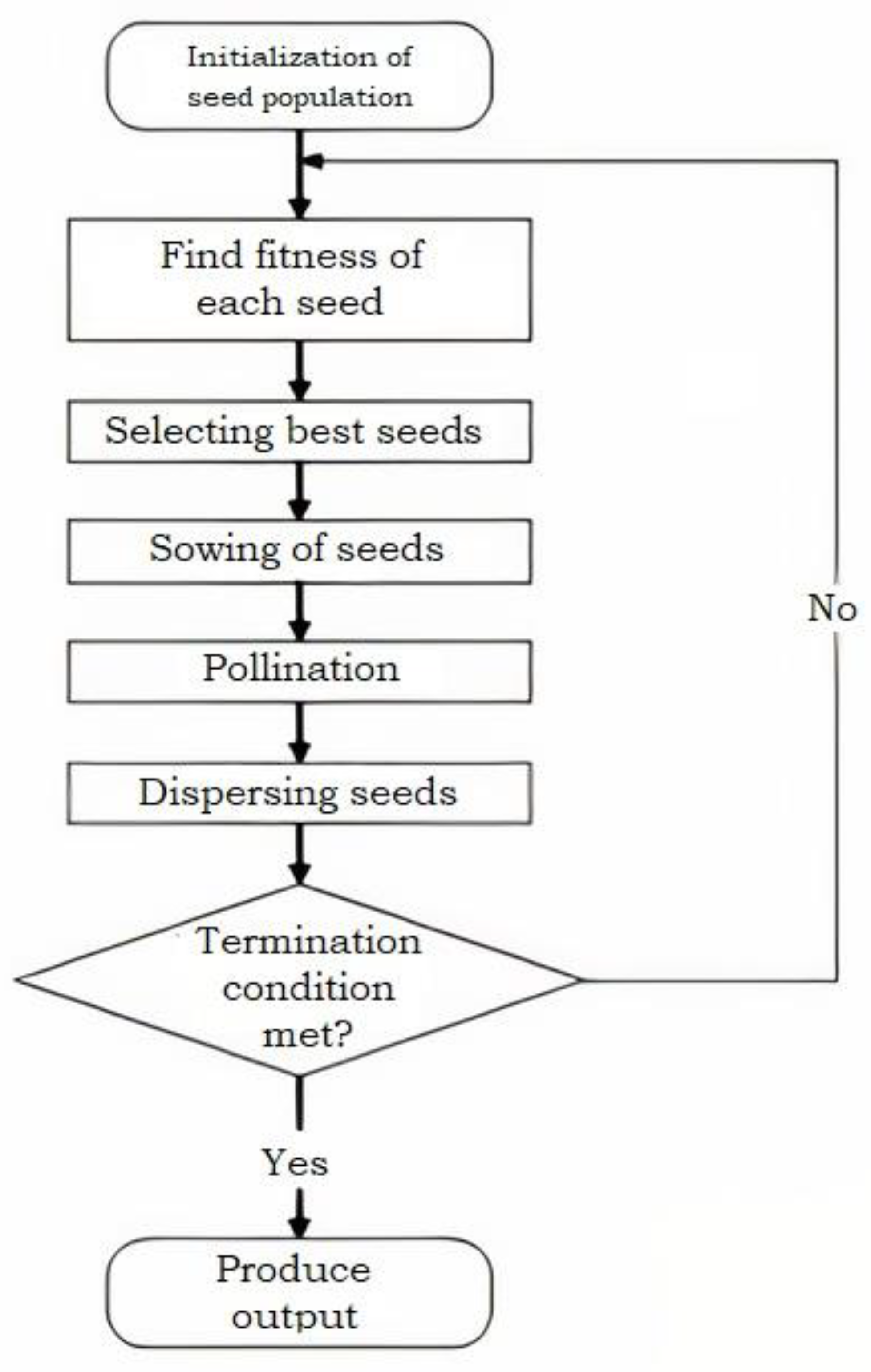
4. Paddy Field Algorithm

Metaheuristic optimization concerns the use of metaheuristic techniques to solve optimization problems. From engineering to economics, optimization happens almost everywhere. Because money, resources, and time are all finite, making the best use of what is available is critical.
Under varied and difficult constraints, most optimizations are highly nonlinear and multimodal. For a single neural network, different hyperparameters might frequently be at odds. Even for a single goal, there are situations when optimal solutions do not exist. Finding an ideal or even sub-optimal solution is not an easy undertaking, in general.
The paddy field algorithm (PFA) is a metaheuristic that is used to search for the best individuals out of a generated population [31]. It was introduced by Premaratne et al. in 2009, inspired by the biological process of pollination in the seeds of a rice crop [32]. As shown in Figure 1, the paddy field algorithm decides the best solution to a problem, just as seeds spread themselves over a growing area to find the most suitable places to root.
When one paddy crop grows in an area, the future generations of that crop are decided based on fitness, due to pollination. Some seeds distribute in the neighboring areas and the viability of those seeds is at maximum, with maximum fitness. A seed with lesser fitness will produce inferior seeds when it grows. This process repeats until the most optimal population of paddy seeds is established [33]. To avoid the possibility of getting caught in a local optimum, seeds are dispersed widely to search for better spaces. This ensures that most of the search space is searched by the Algorithm 1.
Algorithm 1. Paddy Field Algorithm
Step 1:
Initialize a random population of seeds
Step 2:
Calculate the fitness of each seed as:
s = q m a x [ y y t y m a x y t ]
where the maximum fitness value is expressed as max y, y indicates the fitness value of seeds and y t indicates the threshold.
Step 3:
Sort the seeds, in order of fitness.
Step 4:
Produce seeds from the best individuals, where the best fits produce more seeds.
Step 5:
Pollinate seeds in the neighboring space:
S v = U * s
where 0 U 1 . Given a circle of radius a, for two plants Xj and Xk, they will be neighbors to each other if they meet the criteria in Equation (10); thus, determining the neighbor number vj of each plant and the maximum neighbor number of the plant in the same generation, which is expressed as vmax is Equation (11):
u ( X j , X k ) = | X j X k | a < 0
U j = e [ v j v m a x 1 ]
Step 6:
Disperse the plants:
According to Gaussian distribution, the next generation of seeds produced by each plant is scattered within the parameter space; the positions of the seeds are expressed as:
X s e e d i + 1 = N ( x i , σ )
where σ is the coefficient of dispersion, which can determine the dispersion degree of the produced seeds.
Step 7:
Reach termination if one of the termination conditions is met. Otherwise, repeat from Step 2. The termination condition that we used was a time boundary of 8 h.
  S m a x = S 1 * S 2 S n     :   E ( n ) < 480   min
E(n) is the event after n iterations.
Step 8:
Produce output as Smax, when the termination condition is met.
We can also perform a pattern search in the given algorithm if we have enough computing resources.

5. Dataset Pre-Processing

For this study, we used the Google Landmarks dataset, available at https://www.kaggle.com/c/landmark-recognition-2021 (accessed on 22 February 2022) for performing the network architecture search (NAS). This is a dataset comprising around 1.59 M images, including the ones shown in Figure 2. However, training on such a huge dataset would have taken an extremely long time. Therefore, for the evolution of our network, we used only 600 images out of the dataset. It was also noted that one landmark class had a much smaller number of images; hence, the data was augmented 15 times to about 9000 images. The data was augmented in terms of translation, rotation, scaling. cropping. flipping, etc. Augmentation paved the way for an improved generalization of the neural network.
Each picture was checked to make sure that it was in an RGB color encoding scheme, to ensure proper dimensions in terms of colors [34]. After this process, each picture was checked to make sure that it was the same size (64 × 64). An image of inappropriate size was resized to the given dimensions.
Then, the entire dataset was processed so that the input variable had the tensor of the shape:
x = (9000,64,64,3)
The output tensor had the shape:
y = (9000,24)
This meant that the input tensor had 110,592,000 parameters in total. The output had to be one out of 24 classes, as depicted by the output tensor. The dataset was converted into the input tensor variable, while the output tensor was assigned one out of 0–23 numbers for each of the 9000 images. After this, the x tensor and y tensor were used for training. The TensorFlow library provided by Google was imported for creating tensors. However, the overall algorithm was self-designed.

6. Experimentation and Results

We ran the experiment on an Asus VivoBook S15 laptop with 8 GB RAM, a 4 GB NVIDIA graphics card, and an Intel CORE i7 processor. A self-designed code was run in a loop indefinitely for 8 h. In the code, a 3-layer CNN was designed that was then evolved with the paddy field algorithm, and the results were observed.
As shown in Figure 3, the designed CNN consisted of three convolutional layers that were then followed by three max-pooling layers, all of which were then followed by a fully connected layer, with 100 neurons that were varied afterward and 200 neurons that were kept constant.
In Equations (4)–(7), T and F stand for True and False, respectively, while Cn stands for nth class. Accuracy is one of the performance parameters which decide the goodness of a CNN. The complete list of hyperparameters that were evolved can be described as:
  • Kernel Frame Size: the 3 × 3 kernel frames are considered highly optimal for CNNs. However, varying the kernel frame size, we saw that a size of 7 × 7 was the kernel with the best fit of seed. This performed the best with other arrangements of hyperparameters [35]. The kernel frame sizes chosen were between 1 × 1 and 11 × 11. These were in the form of square matrices.
  • Number of Kernels: the number of kernels was varied to establish the best number that could be checked to fall between 22 and 42. It has been suggested that 32 or 64 kernels seem to work well but, for us, 42 was the variant giving the best seed [36]. Other numbers could have worked even better, had we increased the search space.
  • Learning Rate: the learning rate refers to the speed with which the network trains itself. With a slower learning rate, a network can achieve better accuracy, but this increases its chances of running into a local minimum. The network also takes more time to run. A fast learning rate will quicken the rate of learning but run into the problem of deviation from the global minima. A learning rate of 0.01 is considered optimal in the usual cases; indeed, 0.099 was the best parameter found [37]. The learning rate varied between 0.001 and 0.99.
  • Batch Size: the batch size refers to the number of images given to the network for training in one go. A batch size of 32 is considered good; in this case, it was found that 32 is optimal and seemed to perform well [38]. A little variation was found to be good in the batch size, which included 33 and 34 even though it varied between 22 and 42.
  • Neurons: Neurons were also varied to check for the best types of connections. The initial 100 neurons were altered to fall between 90 and 110; the results showed that many variations within this range seemed to do well, although the eventual best fit was 102 [39].
When the CNN was run, the backpropagation ran in the following form:
W x n e w = W x o l d a d ( E r r o r ) d W x
where W x n e w are the newly trained weights, W x o l d are the old weights, a is the learning rate, and a d ( E r r o r ) d W x is the change in an error with respect to the weights. It was run with an AdaDelta optimizer, using the Keras in-built libraries for the optimal changes of weights [40,41,42].
In the code, the CNN hyperparameters were replaced with variables; these variables were initially assigned default CNN hyperparameter values. The accuracy was measured first, then these variables were varied by means of the paddy field algorithm in the search space formed, and the accuracies were consistently recorded. The best seed found, based on accuracy, was [7, 42, 0.0099, 32, 102]. This was in the format of [kernel frame length, number of kernels, learning rate, batch size, neurons] [43,44,45,46].
Figure 4 describes how the maximum accuracy of the evolved networks developed over the elapsed time. Figure 5 shows the accuracy of checked seeds as time progresses. This gives an idea of how the accuracy changes according to the number of seeds that were checked. Figure 6 shows how the accuracy changes from start to finish, as time progresses, when a default CNN is compared to an evolved CNN.
Table 1 gives an insight into how well the self-designed PFANET fared, when compared to a regular CNN with default hyperparameters. Each network has been compared on the basis of the approximate accuracy gained by each network over time. As is apparent, the best-fit PFANET variant gains more accuracy in shorter time frames, compared to a regular CNN. The key observations that should be made are:
  • The best kernel frame length is 7, while the length that was normally used was a 3. 5 kernel frame length, which also performed better than 3 in some combinations. One striking observation was that an unusual kernel frame length of 4, which is not expected to be good because of its being an even kernel frame, also performed better in many regards.
  • The number of kernels after optimization was 42, within the range of 22–42, meaning that the maximum number of kernels improved the model’s accuracy. However, more research would be required to validate how many kernels are optimum.
  • The learning rate that is usually used is 0.01; there was a positive observation that the best learning rate came out to be 0.0099, which is almost 0.01.
  • The number of optimum epochs is 100, but that figure was chosen manually since the network did not then require much processing power at once.
  • The best batch size that was seen was the regularly used size of 32.
  • The neurons did not seem to vary a great deal; the best number was 102 when initialized with 100.
  • The code was run for 8 h and as many as 18 seeds were checked, over a wide variety of combinations.
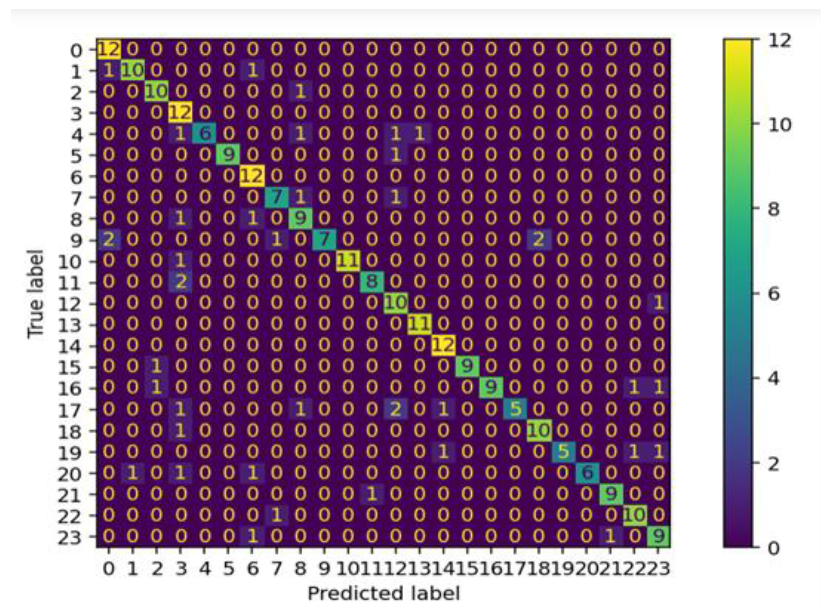
  • In 18 seeds only, the accuracy improved considerably, from 53%, with the default CNN, to 76%.
  • The experiment showed that the paddy field search algorithm is a very viable evolutionary metaheuristic for searching best-fit hyperparameters.
Figure 7 shows the confusion matrix developed for the trained CNN using the evolved hyperparameters. Table 2 shows the best-evolved hyperparameters. The study demonstrated that there can be a high level of change in the performance of a CNN when evolved with an evolutionary metaheuristic, such as the paddy field algorithm.

7. Conclusions

We have demonstrated how to evolve a convolutional neural network using the paddy field algorithm (PFA). We concluded that there is a wide hyperparametric space in which to search for the best combination in a CNN; evolutionary metaheuristics help us to find the best possible combinations in this wide search space. It was found that high performance was recorded using the hyperparameters found by the paddy field algorithm; the accuracy improved a great deal once the CNN was trained. We also concluded that the hyperparameters we employed, which are very different from the hyperparameters that are regularly used, performed much better. We drew a comparison between a default CNN and our evolved CNN; the evolved CNN or PFANET seemed to perform much better. However, more research is required to establish if a particular hyperparameter can work with all combinations. Moreover, the evolution of a network can take too much time for some applications; therefore, we need to improve these algorithms to evolve the ANNs quickly and with stable hyperparameters. Data augmentation helps in the overall improvement of a network.

Author Contributions

K.B.: Conceptualization, Software, Writing: Original Draft, Review and Editing. A.S.: Validation, Formal Analysis, Investigation. S.V.: Resources, Visualization. K.: Project Administration. N.Z.J.: Project Administration, Investigation, Fund Acquisition. M.S.: Fund Acquisition, Software. M.M.: Investigation, Fund Acquisition. All authors have read and agreed to the published version of the manuscript.

Funding

This work was supported by the Taif University Researchers Supporting Project number (TURSP-2020/79), Taif University, Taif, Saudi Arabia.

Acknowledgments

This work was supported by the Taif University Researchers Supporting Project number (TURSP-2020/79), Taif University, Taif, Saudi Arabia.

Conflicts of Interest

The authors declare no conflict of interest.

References

  1. Radenović, F.; Tolias, G.; Chum, O. Fine-tuning CNN image retrieval with no human annotation. IEEE Trans. Pattern Anal. Mach. Intell. 2018, 41, 1655–1668. [Google Scholar] [CrossRef] [PubMed] [Green Version]
  2. LeCun, Y.; Bengio, Y. Convolutional networks for images, speech, and time series. Handb. Brain Theory Neural Netw. 1995, 3361, 1995. [Google Scholar]
  3. Rafiq, M.Y.; Bugmann, G.; Easterbrook, D.J. Neural network design for engineering applications. Comput. Struct. 2001, 79, 1541–1552. [Google Scholar] [CrossRef]
  4. Liu, Y.; Sun, Y.; Xue, B.; Zhang, M.; Yen, G.G.; Tan, K.C. A survey on evolutionary neural architecture search. In IEEE Transactions on Neural Networks and Learning Systems; IEEE: Piscatway, NJ, USA, 2021. [Google Scholar] [CrossRef]
  5. Yang, X.-S. Nature-Inspired Metaheuristic Algorithms; Luniver Press: Beckington, UK, 2010. [Google Scholar]
  6. Hochba, D.S. Approximation algorithms for NP-hard problems. ACM Sigact News 1997, 28, 40–52. [Google Scholar] [CrossRef]
  7. Kong, X.; Chen, Y.-L.; Xie, W.; Wu, X. A novel paddy field algorithm based on pattern search method. In Proceedings of the 2012 IEEE International Conference on Information and Automation, Shenyang, China, 6–8 June 2012; pp. 686–690. [Google Scholar]
  8. Weyand, T.; Araujo, A.; Cao, B.; Sim, J. Google landmarks dataset v2-a large-scale benchmark for instance-level recognition and retrieval. In Proceedings of the IEEE/CVF Conference on Computer Vision and Pattern Recognition, Seattle, WA, USA, 14–19 June 2020; pp. 2575–2584. [Google Scholar]
  9. Bansal, K.; Rana, A.S. Landmark Recognition Using Ensemble-Based Machine Learning Models. In Machine Learning and Data Analytics for Predicting, Managing, and Monitoring Disease; IGI Global: Hershey, PA, USA, 2021; pp. 64–74. [Google Scholar]
  10. Xu, D.; Tu, K.; Wang, Y.; Liu, C.; He, B.; Li, H. FCN-engine: Accelerating deconvolutional layers in classic CNN processors. In Proceedings of the International Conference on Computer-Aided Design, San Diego, CA, USA, 5–8 November 2018; pp. 1–6. [Google Scholar]
  11. Ghosh, S.; Singh, A. Image Classification Using Deep Neural Networks: Emotion Detection Using Facial Images. In Machine Learning and Data Analytics for Predicting, Managing, and Monitoring Disease; IGI Global: Hershey, PA, USA, 2021; pp. 75–85. [Google Scholar]
  12. Hernández, H.; Blum, C. Distributed graph coloring: An approach based on the calling behavior of Japanese tree frogs. Swarm Intell. 2012, 6, 117–150. [Google Scholar] [CrossRef] [Green Version]
  13. Lin, Y.-S.; Lu, H.-C.; Tsao, Y.-B.; Chih, Y.-M.; Chen, W.-C.; Chien, S.-Y. Gratetile: Efficient sparse tensor tiling for CNN processing. In Proceedings of the 2020 IEEE Workshop on Signal Processing Systems (SiPS), Coimbra, Portugal, 20–22 October 2020; pp. 1–6. [Google Scholar]
  14. Wang, M.; Lu, S.; Zhu, D.; Lin, J.; Wang, Z. A high-speed and low-complexity architecture for softmax function in deep learning. In Proceedings of the 2018 IEEE Asia Pacific Conference on Circuits and Systems (APCCAS), Chengdu, China, 26–30 October 2018; pp. 223–226. [Google Scholar]
  15. Bottou, L. Stochastic gradient descent tricks. In Neural Networks: Tricks of the Trade; Springer: Berlin/Heidelberg, Germany, 2012; pp. 421–436. [Google Scholar]
  16. Lydia, A.; Francis, S. Adagrad—An optimizer for stochastic gradient descent. Int. J. Inf. Comput. Sci. 2019, 6, 566–568. [Google Scholar]
  17. Ruder, S. An overview of gradient descent optimization algorithms. arXiv 2016, arXiv:1609.04747. [Google Scholar]
  18. Zhang, Z. Improved adam optimizer for deep neural networks. In Proceedings of the 2018 IEEE/ACM 26th International Symposium on Quality of Service (IWQoS), Banff, AB, Canada, 4–6 June 2018; pp. 1–2. [Google Scholar]
  19. Wang, D.; Wang, X.; Kim, M.-K.; Jung, S.-Y. Integrated optimization of two design techniques for cogging torque reduction combined with analytical method by a simple gradient descent method. IEEE Trans. Magn. 2012, 48, 2265–2276. [Google Scholar] [CrossRef]
  20. Wichrowska, O.; Maheswaranathan, N.; Hoffman, M.W.; Colmenarejo, S.G.; Denil, M.; Freitas, N.; Sohl-Dickstein, J. Learned optimizers that scale and generalize. In Proceedings of the 34th International Conference on Machine Learning, Sydney, NSW, Australia, 6–11 August 2017; pp. 3751–3760. [Google Scholar]
  21. Jafarian, A.; Nia, S.M.; Golmankhaneh, A.K.; Baleanu, D. On artificial neural networks approach with new cost functions. Appl. Math. Comput. 2018, 339, 546–555. Available online: https://EconPapers.repec.org/RePEc:eee:apmaco:v:339:y:2018:i:c:p:546-555 (accessed on 20 February 2022). [CrossRef]
  22. Raja, M.A.Z.; Shah, F.H.; Tariq, M.; Ahmad, I. Design of artificial neural network models optimized with sequential quadratic programming to study the dynamics of nonlinear Troesch’s problem arising in plasma physics. Neural Comput. Appl. 2018, 29, 83–109. [Google Scholar] [CrossRef]
  23. Kumar, S.; Singh, A.; Walia, S. Parallel Big Bang–Big Crunch Global Optimization Algorithm: Performance and its Applications to routing in WMNs. Wirel. Pers. Commun. 2018, 100, 1601–1618. [Google Scholar] [CrossRef]
  24. Sabir, Z.; Raja, M.A.Z.; Guirao, J.L.G.; Saeed, T. Swarm Intelligence Procedures Using Meyer Wavelets as a Neural Network for the Novel Fractional Order Pantograph Singular System. Fractal Fract. 2021, 5, 277. [Google Scholar] [CrossRef]
  25. Boiarov, A.; Tyantov, E. Large scale landmark recognition via deep metric learning. arXiv 2019, arXiv:1908.10192v3. [Google Scholar]
  26. Kumar, S.; Walia, S.S.; Singh, A. Parallel big bang-big crunch algorithm. Int. J. Adv. Comput. 2013, 46, 1330–1335. [Google Scholar]
  27. Singh, A.; Kumar, S.; Walia, S.S.; Chakravorty, S. Face Recognition: A Combined Parallel BB-BC & PCA Approach to Feature Selection. Int. J. Comput. Sci. Inf. Technol. 2015, 2, 1–5. [Google Scholar]
  28. Singh, A.; Kumar, S.; Walia, S.S. Parallel 3-Parent Genetic Algorithm with Application to Routing in Wireless Mesh Networks. In Implementations and Applications of Machine Learning; Springer: Cham, Switzerland, 2020; pp. 1–28. [Google Scholar]
  29. Singh, P.; Chaudhury, S.; Panigrahi, B.K. Hybrid MPSO-CNN: Multi-level Particle Swarm optimized hyperparameters of Convolutional Neural Network. Swarm Evol. Comput. 2021, 63, 100863. [Google Scholar] [CrossRef]
  30. He, X.; Wang, Y.; Wang, X.; Huang, W.; Zhao, S.; Chen, X. Simple-Encoded evolving convolutional neural network and its application to skin disease image classification. Swarm Evol. Comput. 2021, 67, 100955. [Google Scholar] [CrossRef]
  31. Muppala, C.; Guruviah, V. Detection of leaf folder and yellow stemborer moths in the paddy field using deep neural network with search and rescue optimization. Inf. Process. Agric. 2021, 8, 350–358. [Google Scholar] [CrossRef]
  32. Premaratne, U.; Samarabandu, J.; Sidhu, T. A new biologically inspired optimization algorithm. In Proceedings of the 2009 International Conference on Industrial and Information Systems (ICIIS), Peradeniya, Sri Lanka, 28–31 December 2009; pp. 279–284. [Google Scholar]
  33. Zhao, L.; Kobayasi, K.; Hasegawa, T.; Wang, C.L.; Yoshimoto, M.; Wan, J.; Matsui, T. Traits responsible for variation in pollination and seed set among six rice cultivars grown in a miniature paddy field with free air at a hot, humid spot in China. Agric. Ecosyst. Environ. 2010, 139, 110–115. [Google Scholar] [CrossRef]
  34. Magliani, F.; Bidgoli, N.M.; Prati, A. A location-aware embedding technique for accurate landmark recognition. In Proceedings of the 11th International Conference on Distributed Smart Cameras, Stanford, CA, USA, 5–7 September 2017. [Google Scholar]
  35. Ullah, F.U.M.; Ullah, A.; Muhammad, K.; Haq, I.U.; Baik, S.W. Violence detection using spatiotemporal features with 3D convolutional neural network. Sensors 2019, 19, 2472. [Google Scholar] [CrossRef] [Green Version]
  36. Li, Y.; Lin, S.; Zhang, B.; Liu, J.; Doermann, D.; Wu, Y.; Huang, F.; Ji, R. Exploiting kernel sparsity and entropy for interpretable CNN compression. In Proceedings of the IEEE/CVF Conference on Computer Vision and Pattern Recognition, Long Beach, CA, USA, 16–20 June 2019; pp. 2800–2809. [Google Scholar]
  37. Zhuangzhuang, T.; Ronghui, Z.; Jiemin, H.; Jun, Z. Adaptive learning rate CNN for SAR ATR. In Proceedings of the 2016 CIE International Conference on Radar (RADAR), Guangzhou, China, 10–13 October 2016; pp. 1–5. [Google Scholar]
  38. Radiuk, P.M. Impact of training set batch size on the performance of convolutional neural networks for diverse datasets. Inf. Technol. Manag. Sci. 2017, 20, 20–24. [Google Scholar] [CrossRef]
  39. Aizenberg, N.N.; Aizenberg, I.N. Fast-convergence learning algorithms for multi-level and binary neurons and solution of some image processing problems. In International Workshop on Artificial Neural Networks; Springer: Berlin/Heidelberg, Germany, 1993; pp. 230–236. [Google Scholar]
  40. Dogra, V. Banking news-events representation and classification with a novel hybrid model using DistilBERT and rule-based features. Turk. J. Comput. Math. Educ. 2021, 12, 3039–3054. [Google Scholar]
  41. Srivastava, A.; Verma, S.; Jhanjhi, N.Z.; Talib, M.N.; Malhotra, A. Analysis of Quality of Service in VANET. In IOP Conference Series: Materials Science and Engineering; IOP Publishing: Bristol, UK, 2020; Volume 993, p. 012061. [Google Scholar]
  42. Kumar, P.; Verma, S. Detection of Wormhole Attack in VANET. Natl. J. Syst. Inf. Technol. 2017, 10, 71–80. [Google Scholar]
  43. Jhanjhi, N.Z.; Verma, S.; Talib, M.N.; Kaur, G. A Canvass of 5G Network Slicing: Architecture and Security Concern. In IOP Conference Series: Materials Science and Engineering; IOP Publishing: Bristol, UK, 2020; Volume 993, p. 012060. [Google Scholar]
  44. Gandam, A.; Sidhu, J.S.; Verma, S.; Jhanjhi, N.Z.; Nayyar, A.; Abouhawwash, M.; Nam, Y. An efficient post-processing adaptive filtering technique to rectifying the flickering effects. PLoS ONE 2021, 16, e0250959. [Google Scholar] [CrossRef]
  45. Puneeta, S.; Sahil, V. Analysis on Different Strategies Used in Blockchain Technology. J. Comput. Theor. Nanosci. 2019, 16, 4350–4355. [Google Scholar] [CrossRef]
  46. Kumar, K.; Verma, S.; Jhanjhi, N.Z.; Talib, M.N. A Survey of The Design and Security Mechanisms of The Wireless Networks and Mobile Ad-Hoc Networks. In IOP Conference Series: Materials Science and Engineering; IOP Publishing: Bristol, UK, 2020; Volume 993, p. 012063. [Google Scholar]
Figure 1. The complete process followed in the paddy field algorithm [7].
Electronics 11 01075 g001
Figure 2. Landmark images from the Google Landmarks Dataset V2 [8].
Electronics 11 01075 g002
Figure 3. The basic architecture of the designed CNN.
Electronics 11 01075 g003
Figure 4. Accuracies of the evolved PFANET variants as the time elapsed.
Electronics 11 01075 g004
Figure 5. Accuracies for the evolved seeds in the network.
Electronics 11 01075 g005
Figure 6. Accuracy change in evolved CNN vs. Default CNN.
Electronics 11 01075 g006
Figure 7. Confusion matrix for the trained model.
Electronics 11 01075 g007
Table 1. Accuracies in a default CNN and the network evolved with PFA are compared over best fits, shown as the steps of time and epochs elapsed.
Accuracy
S. No.EpochsTime (in mins.)Default CNN (Approx. in %)PFANET (Best Fit) (Approx. in %)
1135812
225101624
338152435
450203145
563253755
675304363
788354870
8100405376
Table 2. The best-fitted seed after the evolution of the CNN architecture with PFA.
Kernel Frame LengthNumber of KernelsLearning RateBatch SizeNeurons
7420.009932102
Publisher’s Note: MDPI stays neutral with regard to jurisdictional claims in published maps and institutional affiliations.

