Selection and Optimization of Hyperparameters in Warm-Started Quantum Optimization for the MaxCut Problem

Abstract

Today’s quantum computers are limited in their capabilities, e.g., the size of executable quantum circuits. The Quantum Approximate Optimization Algorithm (QAOA) addresses these limitations and is, therefore, a promising candidate for achieving a near-term quantum advantage. Warm-starting can further improve QAOA by utilizing classically pre-computed approximations to achieve better solutions at a small circuit depth. However, warm-starting requirements often depend on the quantum algorithm and problem at hand. Warm-started QAOA (WS-QAOA) requires developers to understand how to select approach-specific hyperparameter values that tune the embedding of classically pre-computed approximations. In this paper, we address the problem of hyperparameter selection in WS-QAOA for the maximum cut problem using the classical Goemans–Williamson algorithm for pre-computations. The contributions of this work are as follows: We implement and run a set of experiments to determine how different hyperparameter settings influence the solution quality. In particular, we (i) analyze how the regularization parameter that tunes the bias of the warm-started quantum algorithm towards the pre-computed solution can be selected and optimized, (ii) compare three distinct optimization strategies, and (iii) evaluate five objective functions for the classical optimization, two of which we introduce specifically for our scenario. The experimental results provide insights on efficient selection of the regularization parameter, optimization strategy, and objective function and, thus, support developers in setting up one of the central algorithms of contemporary and near-term quantum computing.

1. Introduction

Quantum computing promises to solve a variety of problems, e.g., in chemistry [1], machine learning [2,3,4,5,6,7,8], or combinatorial optimization [9,10], more efficiently than any classical computer. However, the current generation of gate-based quantum hardware, e.g., based on superconducting qubits [11,12] or trapped ions [13,14], is still deficient in many respects. For instance, the gate and measurement operations are error-prone and the number of qubits, their connectivity, and the maximum depth of executable quantum circuits are limited [15]. A promising candidate for reaching a near-term quantum advantage despite the limitations of these so-called Noisy Intermediate-Scale Quantum (NISQ) devices [16] is the Quantum Approximate Optimization Algorithm (QAOA) [17], a generic algorithm for the approximation of optimal solutions to combinatorial problems. Being a variational quantum algorithm [18], QAOA involves a classical optimization loop to determine parameter values for the QAOA quantum circuit. The approximation quality of QAOA improves theoretically with the number of repetitions, p, of a cost and mixing operator in the quantum circuit. However, since the circuit depth increases linearly with each repetition, the limits for the executability on NISQ devices are reached with only a few repetitions. For example, $p\le 3$ is realistic for reasonably sized problems on current quantum devices [10].

Warm-starting is an approach in classical computing to speed up the search for an optimal solution, which is commonly used in the domains of machine learning and optimization [19,20,21,22,23,24,25]. The general idea is to first generate a rough estimate close to the optimal solution using an efficient algorithm, and then utilize this solution as a starting point for another, more precise algorithm to compute a better approximation. In the context of quantum computing, warm-starting can help achieve better results with limited quantum resources by combining classical and quantum computation in hybrid quantum–classical algorithms [26]. One example application scenario is the warm-started variants of QAOA (WS-QAOA) for solving the Maximum Cut problem (MaxCut) [27,28]—MaxCut focuses on graph partitioning and has many applications, e.g., in machine learning. For example, in the approach by Egger et al. [27], the well-known Goemans–Williamson Algorithm (GW) [29] is used to classically generate an estimate solution that is encoded into the initial state of QAOA, which has the potential to result in improved solution quality with fewer repetitions.

To leverage the advantages of warm-starting for quantum algorithms such as QAOA, additional challenges related to hyperparameter selection need to be taken into account. For example, the approach by Egger et al. [27] introduces a regularization parameter, $\epsilon$, to tune the deviation of the WS-QAOA algorithm from plain QAOA. However, selecting this parameter is not straightforward, as neither its influence on the solution quality for a given problem instance nor guidelines on how this hyperparameter can be selected to achieve a high solution quality are well-documented. Similar questions might arise in regard to the approach by Tate et al. [28], which allows different rotations before the classically pre-computed solutions are mapped to a quantum state—selecting such a rotation from a given set of possible variants is equivalent to setting a categorical hyperparameter. As a result, providing guidelines on (i) how to set such approach-specific hyperparameters for the encoding of classically pre-computed solutions to achieve high solution quality becomes crucial for researchers and practitioners interested in employing WS-QAOA for their use cases.

Moreover, QAOA itself comes with certain traits that need to be addressed appropriately. One major factor is the increase of complexity of both initialization and classical optimization due to the growth of parameters with each additional repetition in the circuit. Obtaining an improved solution quality is, hence, not guaranteed, due to possible limitations of the classical optimization of circuit parameters. Therefore, it is important to identify (ii) which optimization strategies can cope with the initialization and optimization of many circuit parameters to increase the chances of improving the solution quality with WS-QAOA. Furthermore, although several alternative objective functions for the optimization were evaluated and have proven superior for standard QAOA, the existing approaches of WS-QAOA, e.g., WS-QAOA for MaxCut, focus only on the energy expectation value as an objective value [27,28]. In this context, finding alternative objective functions is especially interesting, since good objective values do not necessarily correlate with a high solution quality [30]. Thus, (iii) understanding whether alternative objective functions can improve the solution quality in WS-QAOA and providing guidelines on using them is another important step for facilitating the usage of WS-QAOA.

In this work, we address these challenges in the context of the approach by Egger et al. [27]. To achieve this, we design and conduct a set of experiments in which we treat the optimization strategies and objective functions together with the regularization parameter $\epsilon$ as hyperparameters to the WS-QAOA algorithm. In particular, we consider a total of three optimization strategies and five objective functions. The conducted experiments focus on executions of WS-QAOA for MaxCut with different hyperparameter settings and problem instances, hence, providing insights on selecting these hyperparameters to achieve a high solution quality. Thereby, the contributions of this work are as follows. We (i) analyze how the regularization parameter $\epsilon$ influences the solution quality depending on the input and objective function used in WS-QAOA and derive possibles strategies to select $\epsilon$. Further, we (ii) present and evaluate two new optimization strategies addressing the complexity of initialization and optimization for low-depth QAOA. Our experiments show that these optimization strategies can improve the solution quality of WS-QAOA for MaxCut compared to the standard optimization strategy. Finally, we (iii) evaluate a set of alternative objective functions in the context of WS-QAOA for MaxCut finding that these alternatives can lead to significantly increased solution quality when compared to the standard energy expectation objective function. Two objective functions are introduced in this work specifically for the warm-starting scenario at hand. The two solution quality measures taken into account are the probability of finding a MaxCut (i.e., an optimal solution) and the probability of finding solutions better than the estimate used to warm-start the algorithm.

The remainder of the paper is structured as follows. Section 2 discusses the related work and Section 3 introduces the relevant background. Section 4 motivates the problem and formulates the research questions. Section 5 describes the research design and experimental setup. The results of the experiments are presented and further discussed in Section 6 and Section 7, respectively. Section 8 concludes this work.

2. Related Work

In this section, we first review work on warm-starting in general and WS-QAOA in particular, then focus on alternative objective functions, and finally on a typical optimization approach in the quantum domain.

2.1. Warm-Starting

The concept of warm-starting is widely spread in mathematical programming [19,20,21,22] and classical optimization [23,24,25]. Warm-starting has been identified as a pattern for hybrid algorithms to induce a quantum-classic split [26]. Specifically in the context of QAOA, it has been introduced by Egger et al. [27] and Tate et al. [28]. WS-QAOA has been applied on a small scale for clustering via MaxCut [31,32].

Egger et al. [27] present variants of WS-QAOA based on continuous and rounded SDP results. For MaxCut, their WS-QAOA is based on a rounded GW solution that is regularized as per Equation (2). The mixer is adjusted such that the ground state of $H_M$ is the initial state. For their variant based on rounded SDP, the mixer is additionally adapted in a way that allows the generation of states that differ from the initial cut as well as retain it by choosing certain parameter values. However, the eigenstate of this mixer no longer corresponds to the prepared biased initial state. Thus, the arguments of Farhi et al. [17] for the convergence of the algorithm to an optimal solution with increasing p no longer apply. Egger et al. [27] therefore rely on the empirical analysis of their approach indicating possible improvements upon GW. We build upon this work, but use the mixer that is compatible with [17]. Other than Egger et al. [27], we also focus on different objective functions and optimization strategies as hyperparameters of the algorithm.

Tate et al. [28] introduce a warm-starting pipeline that initializes QAOA with a low-rank Burer–Monteiro relaxation. Nodes are mapped to the ${\mathbb{R}}^k$, where k is the rank (instead ${\mathbb{R}}^n$ in GW, see Section 3), and the mapping is directly encoded into the quantum state; this is in contrast to Egger et al.’s [27] variant where one concrete solution is encoded into the initial state. Specifically, rank-k solutions for $k\in \{2,3\}$ are considered, since the mapping to the Bloch sphere is simple in these cases. As experiments confirm, this variant of warm-started QAOA can consistently outperform CS-QAOA for small p. During the writing of this manuscript, a generalized version of their approach appeared [33], which, instead of using the standard QAOA mixer, is enabled for arbitrary separable initial states and corresponding mixers. In simulations, this version outperformed CS-QAOA, pure GW, as well as its predecessor.

2.2. Alternative Objective Functions for QAOA

For CS-QAOA, alternative objective functions have been evaluated [30,34]. The Conditional Value-at-Risk (CVaR) objective function [30] is inspired by CVaR as used in finance. It only takes the lower tail of the probability distribution into account. Assuming a list of samples sorted by their associated energy values in ascending order, only the fraction $\alpha$ of the first samples in the list is considered, i.e., CVaR computes the average of the energy values of that fraction. It is thus a generalization of the objective function based on the expectation value ($\alpha =1$) and a trivial objective function that returns the minimum sampled solution ($\alpha \to 0$). On the other hand, the Gibbs objective function [34] inspired by Gibbs free energy in statistical mechanics also focuses on low energy values. It is based on the expectation value of $e^{\eta E}$, where E is the corresponding cut size (interpreted as energy) of the samples, and thus gradually de-emphasizes the probability distribution for lower cut sizes depending on $\eta$. Both approaches introduce hyperparameters, $\alpha$ and $\eta$, respectively, for which practical values need to be determined. Recent work [35] further adapted CVaR by gradually evolving $\alpha$ towards 1 during the optimization. An additional ascending function describes this evolution. This function is thus another hyperparameter. The evaluations of these alternative objective functions show significant advantage over optimization based on the energy expectation value depending on the choice of parameters. We evaluate the CVaR and Gibbs objective functions; however, this was done in the context of WS-QAOA and alongside other alternatives without additional hyperparameters.

2.3. Layer-Wise Training

Layer-wise training or, in other words, step-wise optimization is widely used with VQA and quantum neural networks [36,37,38,39]. The basic idea is to optimize only a portion of the parameters of a parameterized quantum circuit at a time, since training all parameters at once can be very cumbersome for the optimizer, especially in a non-convex parameter space, leading to inferior results. The underlying layer-wise trainability conjecture is proved to not be true in all cases [40], i.e., the optimization can be predestined to saturate prematurely without finding the global optimum. However, very recent work shows that, for QAOA, this saturation occurs only as p reaches closer to the number of qubits [41]. Thus, layer-wise optimization can outperform standard optimization for low-depth QAOA. With what we call incremental optimization, we evaluate very similar optimization strategies in the context of WS-QAOA.

3. Background

In this section, we provide details on the core concepts required for this work, including QAOA and the warm-started variant of QAOA for the MaxCut problem.

3.1. Quantum Algorithms in the NISQ Era

NISQ devices are error-prone and limited in several respects [11,15,16], e.g., the limited number of qubits and their lack of interconnections limit the usage of multi-qubit gates and the size of problems they can solve. Moreover, gates introduce errors to the quantum states as they are executed with insufficient success probability, and qubits quickly lose their states due to decoherence over time. Moreover, interactions with the environment and crosstalk between qubits may, despite all shielding, influence states. Measurement operations themselves are error-prone too, since measurement time is significant compared to the decoherence time of qubits, and thus measurement may not complete before decoherence sets in. These limited capabilities of today’s NISQ devices restrict the width and depth of executable quantum circuits strongly [15,16,42].

To still achieve good results with NISQ devices, hybrid quantum–classical algorithms, i.e., algorithms comprising alternating classical and quantum parts, take advantage of both quantum and classical computers [16]. Essentially, most quantum algorithms are hybrid as they often require pre- and post-processing on classical computers, e.g., classical data need to be encoded into the quantum circuit and post-processing needs to be applied afterwards to retrieve meaningful results from the algorithm [43].

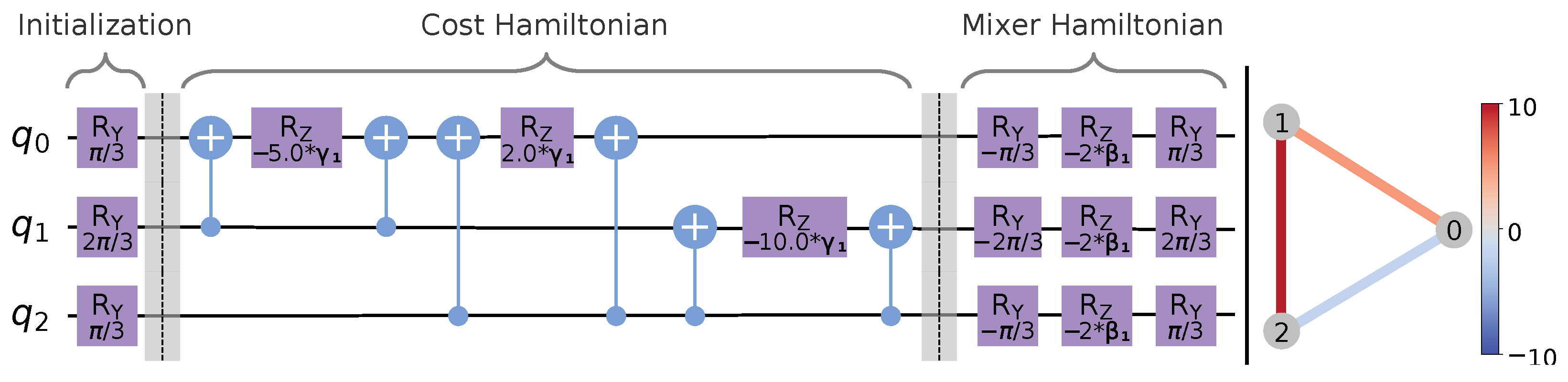
3.2. The Quantum Approximate Optimization Algorithm

Variational Quantum Algorithms (VQA) are hybrid quantum–classical algorithms that utilize a classical optimizer to learn parameters for a parameterized quantum circuit, the so-called ansatz [18]. The goal is to search for (approximate) solutions for problems that are hard to solve on classical computers. The ansätze for a VQA can be categorized as problem-inspired or problem-agnostic, depending on whether information about the problem is incorporated into the ansatz or not. In the case of QAOA, a problem-inspired ansatz is employed, which requires the encoding of a given combinatorial optimization problem into a cost Hamiltonian, $H_C$, that corresponds to the total energy of a system, such that the ground state of $H_C$ corresponds to the optimal solution.

QAOA was first introduced by Farhi et al. [17]. The initial state of the QAOA quantum circuit is the equal superposition of all n qubits, ${|+\rangle }^{\otimes n}$. Apart from $H_C$, a mixer Hamiltonian, $H_M$, is used, the eigenstate of which is ${|+\rangle }^{\otimes n}$, i.e., exactly the initial state. The Hamiltonians are implemented by corresponding unitary operators $U(H_C,{\gamma }_i):=e^{-\mathrm{i}{\gamma }_i{H}_C}$ and $U(H_M,{\beta }_i):=e^{-\mathrm{i}{\gamma }_i{H}_M}$. These operators are employed to implement a trotterized approximation of an adiabatic evolution, thus leveraging the adiabatic theorem—Adiabatic evolution follows the adiabatic theorem to achieve a transition of a system from the known ground state of a Hamiltonian to the unknown ground state of another Hamiltonian, in this case, from the initial state as a ground state of $H_M$ to a ground state of $H_C$, an optimal solution [44]. Therefore, the circuit proceeds from the initial state with sequential applications of $U(H_C,{\gamma }_i)$ and $U(H_M,{\beta }_i)$, where $i\in \{1,\dots ,p\}$ in p repetitions. The parameters ${\gamma }_i,{\beta }_i$ boil down to rotation angles for both operators. As p, and thus the circuit depth, is increased, the approximation quality improves, and the quantum state converges towards a ground state of $H_C$ corresponding to an optimal solution. The parameter values ${\gamma }_i,{\beta }_i$ for $i\in \{1,\dots ,p\}$ are determined using a classical optimizer. The optimizer evaluates the measured result of the executed circuit according to a classical objective function that correlates with the quality of the approximated solution. The original objective function computes the expectation value for the energy of the measured states, that is, by definition of $H_C$, linked with the optimality of the solution.

The potential of QAOA to perform tasks intractable on classical hardware is of great research interest. According to current estimations, such quantum advantage via QAOA can be reached with a few hundred qubits [45]. Further research indicates that the performance of the algorithm strongly depends on a problem density property, e.g., the clause to variable ratio of constraint satisfiability problems [46].

3.3. Warm-Started QAOA for Maximum Cut

As mentioned before, the general idea of warm-starting is to use the knowledge of previous solutions or solutions for related or relaxed problems to facilitate the search for better solutions. Warm-starting does not guarantee finding the best solution efficiently but may speed up the search for a good result. In the context of quantum computing, warm-starting describes the concept of utilizing a classical approximation as an initial point for the quantum algorithm to improve upon [26].

Warm-starting has also been employed by Egger et al. [27] and Tate et al. [28] for one of the most widely used examples [47] for QAOA, the Maximum Cut problem (MaxCut). A cut is a division of an undirected graph into two partitions. It can be seen as a bit string from ${\{0,1\}}^n$ that assigns each of n nodes of the graph to a partition. The number of edges between the nodes of both partitions of a cut is the cut size. In the case of weighted graphs, the sum of the edge weights is considered instead. MaxCut is the problem of finding a cut with the maximum cut size for the respective graph. Such a cut is also referred to as a MaxCut. There can also be different cuts that take the same maximum value. For a given graph with n nodes, the MaxCut cost operator to compute the size of a cut $Z\in {\{0,1\}}^n$ can be defined as:

$$\begin{array}{c}C\left(Z\right)=\sum _{\{i,j\}\in E}{w}_{i,j}(Z_{\left[i\right]}\oplus Z_{\left[j\right]})\\ =\sum _{\{i,j\}\in E}{w}_{i,j}((Z_{\left[i\right]}(1-Z_{\left[j\right]})+Z_{\left[j\right]}(1-Z_{\left[i\right]})),\end{array}$$

(1)

where ⊕ denotes an exclusive or (XOR), $w_{i,j}$ is the weight of an edge $E_{i,j}$, and $Z_{\left[i\right]}$ specifies the assignment of the ith node to one of the two partitions as described above.

Determining the MaxCut is well known to be an NP-hard problem [48]; however, there exist approximation algorithms. In classical computing, GW [29] is the best known algorithm to approximate MaxCut. The algorithm is based on a semi-definite programming (SDP) relaxation with random-hyperplane rounding, i.e., nodes are mapped to unit vectors in ${\mathbb{R}}^n$ and then separated by a random hyperplane through the origin. For graphs with non-negative edge weights, it is known to deliver solutions of an expected cut size that is about ≈87.8% of the MaxCut. Under the Unique Games Conjecture, GW is believed to be the optimal classical algorithm for MaxCut [49]. However, only the NP-hardness of achieving an approximation ratio above ≈94.1% has been proven [50].

For their warm-started variant of QAOA for MaxCut, Egger et al. [27] introduce a regularization parameter, $\epsilon \in [0,0.5]$, to map $0\mapsto \epsilon$ and $1\mapsto 1-\epsilon$ in order to prepare a biased superposition based on a classically pre-computed cut, Z, as the initial state to warm-start QAOA. The biased superposition on each qubit is created by means of an $R_Y$ rotation by an angle $\theta$ according to

$$\begin{array}{ccc}\theta =2·\arcsin \left(\sqrt{\epsilon }\right)\hfill & \hfill & \mathrm{if}{Z}_{\left[i\right]}=0,\hfill \\ \theta =2·\arcsin \left(\sqrt{1-\epsilon }\right)\hfill & \hfill & \mathrm{if}{Z}_{\left[i\right]}=1.\hfill \end{array}$$

(2)

WS-QAOA with $\epsilon =0.5$ results in $\theta =\frac{\pi }{2}$, which initializes all qubits in the $|+\rangle$ state and is equivalent to standard, i.e., cold-started, QAOA (CS-QAOA).

4. Motivation and Research Questions

Solving the problem of finding maximum cuts in graphs is important in various domains, for example, in solid-state physics and very large-scale integrated (VLSI) circuit design [51]. In the former, MaxCut can be used to find ground states of spin glasses, i.e., alloys of magnetic impurities diluted in non-magnetic metal. In VLSI, it is applied to minimize the number of holes on printed circuit boards or contacts on chips. Another application scenario for MaxCut is related to data clustering [52]. The graph partitioning described by MaxCut can be used to separate data points into clusters, e.g., for pattern detection in the domain of digital humanities [53]. While MaxCut can be approximated using the classical GW algorithm, the combination of GW and QAOA into a hybrid warm-started quantum algorithm is promising [27]. Figure 1 shows a developer’s perspective on using WS-QAOA for MaxCut.

First, the data supplied to the algorithm often require pre-processing, e.g., transforming categorical into numerical data to represent it as a graph. Next, the WS-QAOA algorithm needs to be configured with suitable hyperparameter values before executing it. After the execution, the results are post-processed, which can also include reconfiguration of hyperparameters to further improve the result. When compared to classical techniques, such quantum-based, hybrid machine learning methods promise superior results either in accuracy or time consumption, making quantum machine learning (QML) a rapidly evolving research area [2,3,4,5,6,7,8].

Similar to classical machine learning (ML) [54,55], QML algorithms also face the problem of selecting hyperparameters [53]. Furthermore, QML algorithms, which are often hybrid [4,16], introduce additional hyperparameters, such as those related to quantum circuit design and execution aspects. For example, WS-QAOA comes with multiple hyperparameters requiring an in-depth knowledge of the underlying quantum-mechanical aspects of the circuit or extensive testing on scarce quantum devices including cumbersome evaluation of measurements to determine viable values for these parameters. One particular example of such quantum-specific hyperparameters is the regularization parameter $\epsilon$ employed in the approach by Egger et al. [27] (see Section 3). This is a continuous hyperparameter [54] that tunes the bias of the superposition in the initial state towards the classically pre-computed approximation. Since it directly influences the quantum state, the regularization parameter, $\epsilon$, evidently has great potential influence on the state measured after circuit execution and, thus, on the resulting solution quality. Categorical hyperparameters [54], such as strategies employed for optimization and objective functions, used during optimization also influence the solution quality of the algorithm significantly. At the same time, these hyperparameters possess characteristics unique to the quantum computing domain. More specifically, optimization strategies can leverage knowledge of the circuit design to increase the performance of the quantum algorithm and the objective functions need to process measured quantum states to evaluate and direct the optimization progress, thus significantly impacting the resulting solution. For example, the standard objective function evaluates the energy expectation value, i.e., in the case of MaxCut, effectively the expected cut size corresponding to measured states. Therefore, to improve the quality of solutions obtained with WS-QAOA for MaxCut, application developers need to understand the influence of these quantum-specific hyperparameters on the solution quality and know how to configure the algorithm with respect to suitable parameter values.

While the influence of the regularization parameter $\epsilon$ on the energy expectation value has previously been investigated [27], an evaluation of its influence on the solution quality, i.e., the probability of obtaining the MaxCut and cuts better than the classically pre-computed solution, has not been previously studied. For example, instead of indicating an improved solution quality, good energy expectation values can in fact signify that the pre-computed cut has merely been preserved. Moreover, it has not been investigated yet, whether delegating the selection of the regularization parameter $\epsilon$ to classical optimizers is a feasible approach to facilitate the selection process for $\epsilon$, as it is often performed with continuous hyperparameters in classical ML [54]. Thus, it is important to understand how to efficiently select ε values such that the solution quality is increased. Furthermore, since the number of circuit parameters to be adjusted by the optimizer increases with the number of repetitions of the QAOA ansatz, strategies for the initialization and optimization of these parameters are needed to cope with the increasing optimization complexity. Also the time span needed for the parameter optimization may increase with the number of parameters and depending on the optimization strategy. Although optimization strategies from ML could help, they need to be transferred to and evaluated in the context of WS-QAOA for MaxCut, which, has not been previously investigated. Finally, while different objective functions have been studied for QAOA [30,34,35], to the best of our knowledge, their applicability in the context of WS-QAOA for MaxCut is yet to be analyzed. Moreover, these objective functions introduce additional, conditional hyperparameters [54] which need to be configured whenever the respective objective function is selected, hence, making the selection process even more complex. Thus, it is important to understand (i) how existing objective functions can be employed in the context of WS-QAOA for MaxCut and (ii) whether suitable alternative objective functions without additional hyperparameters exist and can be used instead, to simplify the selection of objective functions.

Therefore, to address the aforementioned hyperparameter selection issues in the context of WS-QAOA for MaxCut, we formulate the research questions in this work as follows:

RQ1: 

“How does the regularization parameter ε influence the solution quality, and is it possible and meaningful to delegate the adjustment of ε to a classical optimizer?”

RQ2: 

“How do different optimization strategies for WS-QAOA influence the solution quality and runtime of the optimization?”

RQ3: 

“Which alternative objective functions apart from the energy expectation value are suitable for WS-QAOA, and how do they correlate with the solution quality, and are objective functions without additional hyperparameters practical?”

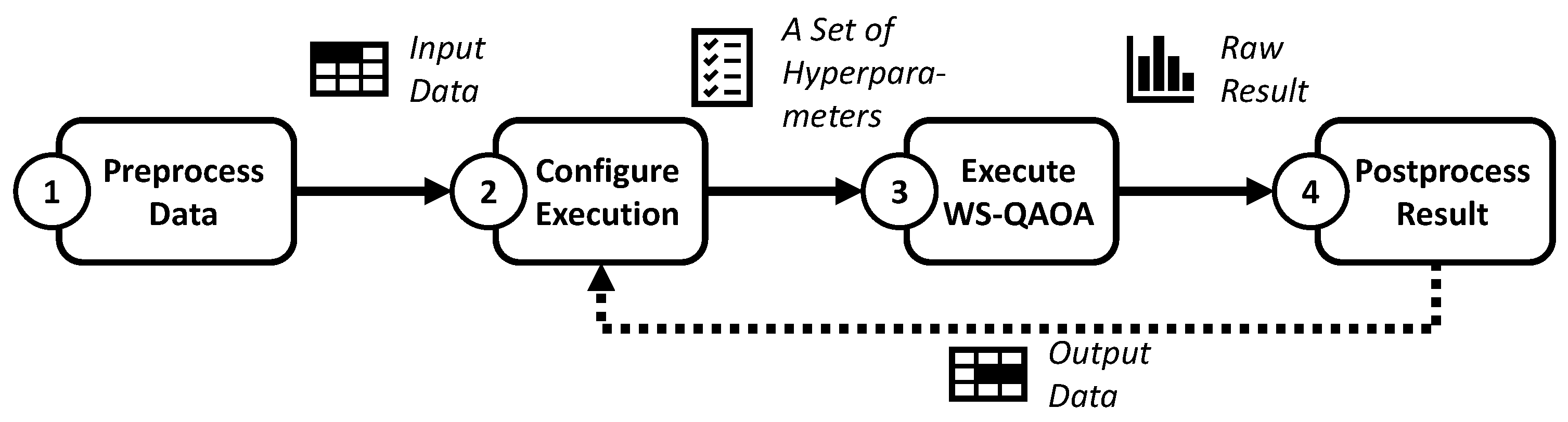
5. Research Design

In this section, we design a set of experiments to address the research questions formulated in Section 4 and discuss the details of the prototypical implementation. Firstly, we give a general overview of the evaluation process and provide the technical details related to its major steps. Afterwards, we describe three experiments that focus on different aspects of hyperparameter selection for WS-QAOA, namely (i) the regularization parameter $\epsilon$, (ii) optimization strategies, and (iii) alternative objective functions.

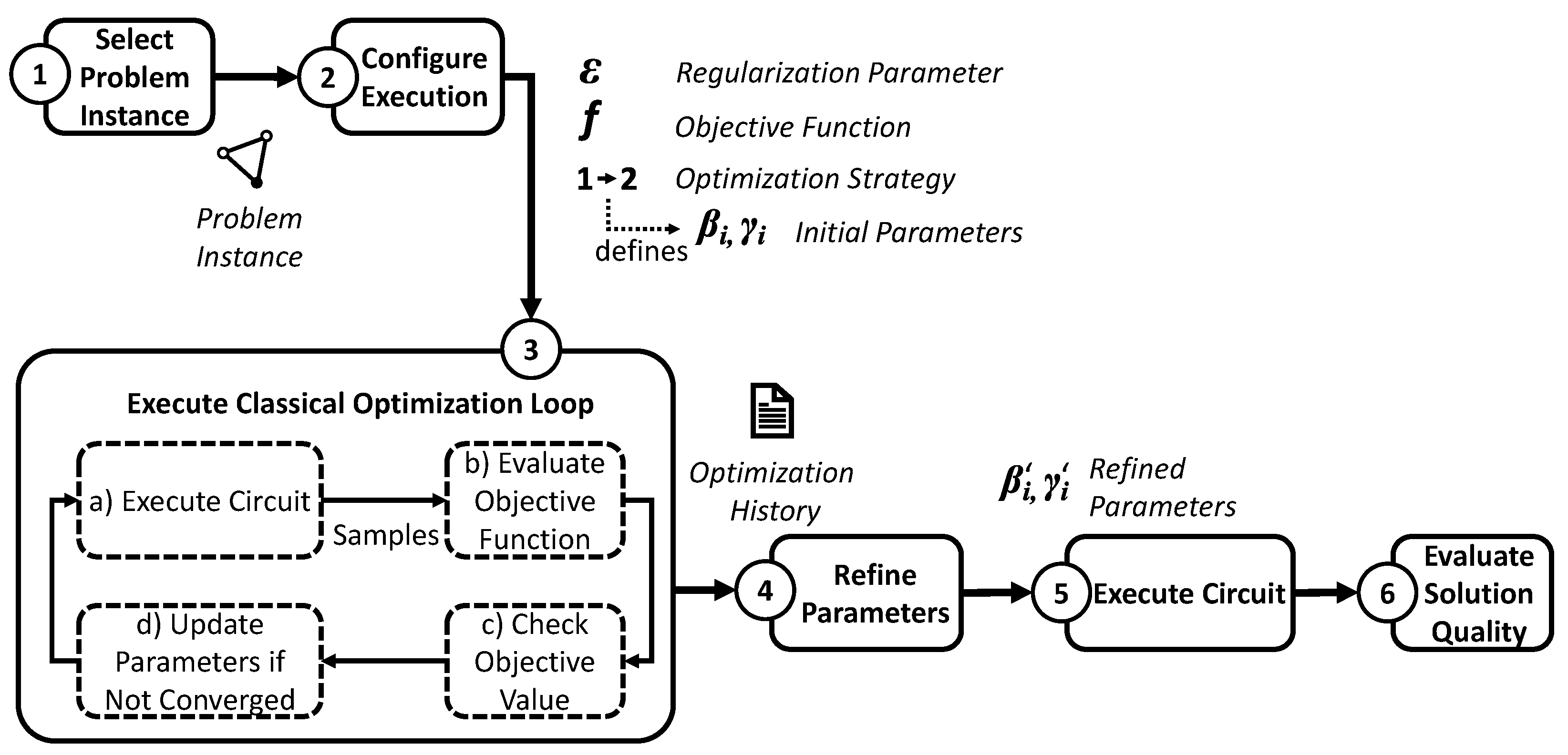
5.1. Overview of the Evaluation Process

To investigate the different aspects of hyperparameter selection defined in the research questions (Section 4), we implement and execute the optimization loop using different hyperparameter settings and evaluate the resulting solution quality as depicted in Figure 2. In Step 1, shown in Figure 2, we select a problem instance. In the case of WS-QAOA for MaxCut, a problem instance is a graph with a given pre-computed initial cut that is used for the warm-starting, i.e., as a starting point, it improves the search for the optimal or an approximate solution. In Step 2, the algorithm needs to be configured for execution. The configuration of an execution involves selecting three kinds of hyperparameters, namely (i) the regularization parameter $\epsilon$, (ii) an optimization strategy, and (iii) an objective function. Additionally, it is worth emphasizing that the choice of an optimization strategy also defines how (iv) the parameters for the quantum circuit, $({\beta }_i,{\gamma }_i)$, are initialized. Next, in Step 3, the optimization loop is executed to maximize the objective value and, hence, increase the size of cuts sampled from the circuit execution by adjusting the circuit parameters ${\beta }_i,{\gamma }_i$. In the optimization loop, a classical optimizer executes the WS-QAOA quantum circuit with iteratively updated parameter values, as shown in Step 3a of Figure 2. The resulting measurements are evaluated according to the configured objective function, as shown in Step 3b. Afterwards, the classical optimizer checks for convergence (Step 3c) and, if the optimization has not converged, continues the iteration with parameters updated according to its internal policy aiming to increase the objective value (Step 3d). When the optimization loop is completed, the refined parameter values need to be retrieved as shown in Step 4 of Figure 2. In this step, we utilize the optimization history to further improve the parameters. Finally, in Step 5, the circuit is executed with these refined parameters and the solution quality evaluated based on the measured samples. In the following, we elaborate on each step of the evaluation process.

➀ Problem Instance Selection. To obtain the problem instances, we generate three regular ($G_{n,\mathit{3}\mathit{r}}$), random ($G_{n,\mathit{rand}}$), and fully-connected graphs ($G_{n,\mathit{fc}}$). For our experiments, we use graphs with $n=12$ and 24 nodes and random edge weights $w_{i,j}\in \{-10,\dots ,10\}$ as depicted in Figure 3.

For random graphs, edges are inserted at random positions: 33 edges for 12-node graphs and 138 edges for 24-node graphs, i.e., half of the maximum possible edges in each case. As the graphs are relatively small, the MaxCut can be determined classically and is, in fact, often also output by the Goemans–Williamson Algorithm (GW). We use GW to pre-compute high-quality starting points (initial cuts) to warm-start QAOA. An excerpt of cuts for the graphs shown in Figure 3 computed using GW is provided in

Table 1. Cuts and MaxCuts of the graphs in Figure 3. Cuts are represented as bit strings as described in Section 3. Those for 12-node graphs are given in the left-hand side and those for 24-node graphs in the right-hand side of the table alongside the cut size and respective ratio of the MaxCut.

Graph	$\mathit{n}=12$			$\mathit{n}=24$
	Cut	Size	$\frac{\mathbf{Size}}{\mathbf{MaxCut}}$	Cut	Size	$\frac{\mathbf{Size}}{\mathbf{MaxCut}}$
$G_{n,\mathit{3}\mathit{r}}$	100010110011	18	1	110111111010011000101000	111	1
	100000100111	16	0.8889	101000000101100111110101	97	0.8739
$G_{n,\mathit{rand}}$	111010100111	98	1	100000001011000111100110	166	1
	101111001010	86	0.8776	100000001010100110010111	145	0.8735
$G_{n,\mathit{fc}}$	111110011010	103	1	110001101001100111001001	278	1
	110010111010	100	0.9709	110011101001110111001001	246	0.8849
	111110111010	92	0.8932
	111110001010	91	0.8835
	111010111010	91	0.8835

with the respective MaxCuts.

➁ Configure Execution. As discussed previously, the selection of objective functions and optimization strategies plays a critical role in improving the solution quality. In the following, we elaborate on the set of optimization strategies and objective functions employed as hyperparamteres during the configuration step for running our experiments.

Selecting the Optimization Strategy. For the configuration step, we employ three optimization strategies, namely (i) the standard optimization strategy and two variants of what we call the incremental optimization strategy—(ii) incremental full optimization and (iii) incremental partial optimization. Inspired by classical optimization approaches [56], the standard optimization strategy is to start directly with the intended QAOA depth and randomly initialize and optimize all circuit parameters at once. In contrast to the standard optimization strategy, the employed incremental optimization strategies focus on step-by-step initialization and optimization inspired by similar approaches for classical and quantum machine learning algorithms [36,37,38,39,57]. To better explain these strategies, we look into the properties of the QAOA circuit. For p repetitions of the QAOA ansatz, the cost Hamiltonian, $H_C$, and mixer Hamiltonian, $H_M$, are repeatedly applied p times and circuit parameters ${\gamma }_i,{\beta }_i$ ($i\in \{1,\dots ,p\}$) are introduced to the circuit. When both ${\gamma }_i$ and ${\beta }_i$ are set to 0 for one repetition of the Hamiltonians, the circuit effectively equals that for $p-1$. Therefore, it is always possible to retain the state generated by a lower-depth QAOA circuit. This immediately suggests building the initialization of parameters on the optimized parameters for a lower-depth WS-QAOA circuit. For instance, in order to optimize the parameters for depth-2 QAOA, one can first find optimal parameters ${\gamma }_1,{\beta }_1$ by running depth-1 QAOA with random initial values. Subsequently, $({\gamma }_1^{\prime },{\beta }_1^{\prime },{\gamma }_2^{\prime },{\beta }_2^{\prime })=({\gamma }_1,{\beta }_1,0,0)$ can be used as initial parameter values for depth-2 QAOA. We consider two options for the optimization from this point: either optimizing all parameters, in this case ${\gamma }_1^{\prime },{\beta }_1^{\prime },{\gamma }_2^{\prime }$, and ${\beta }_2^{\prime }$, or optimizing only the new parameters that were initialized with zeroes, in this case ${\gamma }_2^{\prime }$ and ${\beta }_2^{\prime }$. We call the former variant incremental full optimization and the latter incremental partial optimization. Clearly, incremental partial optimization aims to further simplify the optimization process by reducing the number of parameters to be optimized in a step.

Selecting the Objective Function. For the objective function selection during the configuration step, we employ five objective functions. Three of them are known from the literature, namely (i) $F_{\mathit{EE}}$ based on the energy expectation value [27], (ii) $F_{\alpha ,\mathit{CVaR}}$ inspired by the Conditional Value-at-Risk [30], and (iii) $F_{\eta ,\mathit{Gibbs}}$ inspired by Gibbs energy [34]. Additionally, we introduce two new alternatives, namely (iv) $F_{\mathit{Greedy}}$ and (v) $F_{\mathit{EE}-\mathit{I}}$, which are both adaptations of $F_{\mathit{EE}}$ for our warm-starting scenario. The five objective functions are given by Equations (3)–(7) an explained in more detail below.

$F_{\mathit{EE}}$ is the standard objective function based on the expectation value for the cut size of sampled solutions, which, in other terminology, is considered a representation of an energy value. The cut size is computed by the cost function C as given in Equation (1), $X_i$ is the ith of a total of K sampled solutions, i.e., K is the number of shots for the circuit execution.

$$F_{\mathit{EE}}=\sum _i\frac{C\left(X_i\right)}{K}$$

(3)

$F_{\alpha ,\mathit{CVaR}}$ [30] assumes that the samples $X_i$ are stored in descending order with respect to the associated cost (i.e., $C\left(X_i\right)\ge C\left(X_{i+1}\right)$). The hyperparameter $\alpha$ determines what fraction of a total K samples is considered.

$$F_{\alpha ,\mathit{CVaR}}=\sum _{i=0}^{\lceil \alpha K\rceil }\frac{C\left(X_i\right)}{\lceil \alpha K\rceil }.$$

(4)

For $F_{\eta ,\mathit{Gibbs}}$ [34], $\eta$ is a hyperparameter tuning the exponential profile of the objective function.

$$F_{\eta ,\mathit{Gibbs}}=log\sum _i{e}^{\eta C\left(X_i\right)}·\frac{1}{K}$$

(5)

$F_{\mathit{Greedy}}$ is designed to take into account only samples that yield a cut size above the size of the initial cut $C\left(I\right)$ used to warm-start the optimization. Hence, it is similar to $F_{\alpha ,\mathit{CVaR}}$ but avoids the additional hyperparameter $\alpha$. The intuition behind this objective function is that, with warm-starting, we aim to find cuts that are better than the initial cut and should, therefore, focus only on such cuts.

$$F_{\mathit{Greedy}}=\sum _i\frac{\widehat{C}\left(X_i\right)}{K},\left\{\begin{array}{ccc}\hfill & \widehat{C}=C,\hfill & C\left(X_i\right)>C\left(I\right)\hfill \\ \hfill & \widehat{C}=0,\hfill & \mathrm{else}\hfill \end{array}.\right.$$

(6)

$F_{\mathit{EE}-\mathit{I}}$ merely disregards samples with a cut size equal to that of the initial cut I and, thereby, in contrast to $F_{\mathit{Greedy}}$, also factors in cuts that are worse than I, such that these could be avoided in the optimization.

$$F_{\mathit{EE}-\mathit{I}}=\sum _i\frac{\widehat{C}\left(X_i\right)}{K},\left\{\begin{array}{ccc}\hfill & \widehat{C}=C,\hfill & C\left(X_i\right)\ne C\left(I\right)\hfill \\ \hfill & \widehat{C}=0,\hfill & \mathrm{else}.\hfill \end{array}\right.$$

(7)

➂ Execute Classical Optimization Loop. We follow previous analyses [27,30,58] in using the gradient-free classical optimizer COBYLA via SciPy with the respective default parameters [59]. COBYLA employs a linear approximation approach and supports inequality constraints. The implementation relies on minimizing the negated objective values computed by Equations (3)–(7), which is equivalent to maximization. Therefore, the minimization and maximization problem are not strictly distinguished in this work. When we talk of high objective values as beneficial, the problem is viewed from the maximization perspective although on the implementation level negated objective values are minimized.

➃ Refine Parameters. Traditionally, the classical optimizer returns the final optimized parameters that it determined at the end of the optimization loop. Occasionally, during the optimization process, the optimizer probes parameter values that yield objective values better than achieved with the final optimized parameter output by the optimizer. This may happen especially in non-convex optimization, which is often the case in the $(\gamma ,\beta )$ space for QAOA (we discuss this in more detail when presenting the experimental results in Section 6). While intermediate results are usually discarded during optimization, our strategy is to exploit them for post-optimization parameter refinement by picking the best parameters (as per the corresponding objective values) probed during optimization. This can be seen as a cross between optimization and exhaustive search in the $(\gamma ,\beta )$ space. As a result, this selective parameter refinement using the optimization history provides parameters at least as good as traditional optimization but better results on average.

➄ Execute Circuit for Problem Instance. For both circuit execution steps, occurring inside (Step 3a) and outside (Step 5) of the optimization loop, we define and implement the WS-QAOA quantum circuit. Since each node is represented by one qubit, the circuit width coincides with the number of nodes of the considered graph, i.e., the problem instances (Figure 3) require 12 and 24 qubits, respectively. The principal structure of the quantum circuit is shown in Figure 4 for a minimal example.

It consists of an initialization, the implementation of the cost Hamiltonian $H_C$, and the mixer Hamiltonian $H_M$ (each separated by a barrier in Figure 4). The $R_Y$ rotations in the first section encode the initial cut sequence 010 (cut size: 15) according to Equation (2) using $\epsilon =0.25$. $H_C$ is integrated into the circuit in the second section by adding a (CNOT, $R_Z(-w_{i,j}·{\gamma }_1)$, CNOT) group for each edge, where $w_{i,j}$ is the respective edge weight, and the control and target qubit for CNOT consist of the pair of nodes connected by the edge. The mixer $H_M$ is the adjusted version for WS-QAOA from [27], however, without the additional changes for rounded SDP. It applies a sequence of rotations $R_Y,R_Z,R_Y$ for each qubit in the last section of the circuit, where $R_Y$ depends on the initial state, and $R_Z$ depends on the hyperparameter ${\beta }_1$. Thus, the initial state is an eigenstate of the mixer and the arguments regarding the convergence of the algorithm with the ground state (with increasing p) apply [17]. In case the circuit cannot reproduce the initial cut, it can be retained classically so as to ensure that the algorithm performs at least as well as mere GW. Circuit execution for our experiments is simulated locally on Qiskit’s QasmSimulator backend [60]. In order to obtain reliable information on the probability distribution, 5000 shots are sampled in each circuit execution. The measured bit strings are interpreted as a mapping of the nodes to a partition. For instance, the bit string 010 encodes the MaxCut of the graph depicted in Figure 4, where node 1 is in a different partition, partition 1, than the remaining nodes, which are assigned to partition 0.

➅ Evaluate Solution Quality. We consider the probability of sampling a MaxCut (MaxCut probability) as the main evaluation criterion for the comparison of different hyperparameter settings. It corresponds to the probability of transitioning into a ground state for the cost Hamiltonian and is estimated directly from the fraction of shots that result in such a state. An additional measure is the overall probability of sampling a cut better than the initial cut for WS-QAOA (BetterCut probability), which corresponds to transitions into lower energy states compared to the state corresponding to the initial cut. The latter may be more suitable in some cases where a direct transition into a ground state is highly unlikely, but WS-QAOA can still improve upon the classically pre-computed result.

5.2. Experiment Designs

Having discussed the core aspects of the evaluation process, in the following we design a set of experiments aimed at evaluating how different hyperparameters influence the solution quality for WS-QAOA for the MaxCut problem. Each experiment is designed to answer the corresponding research question formulated in Section 4.

• Experiment 1: Influence of the regularization parameter $\epsilon$

To analyze the influences of the regularization parameter $\epsilon$ on the solution quality as formulated in RQ1 in Section 4, we perform the following steps:

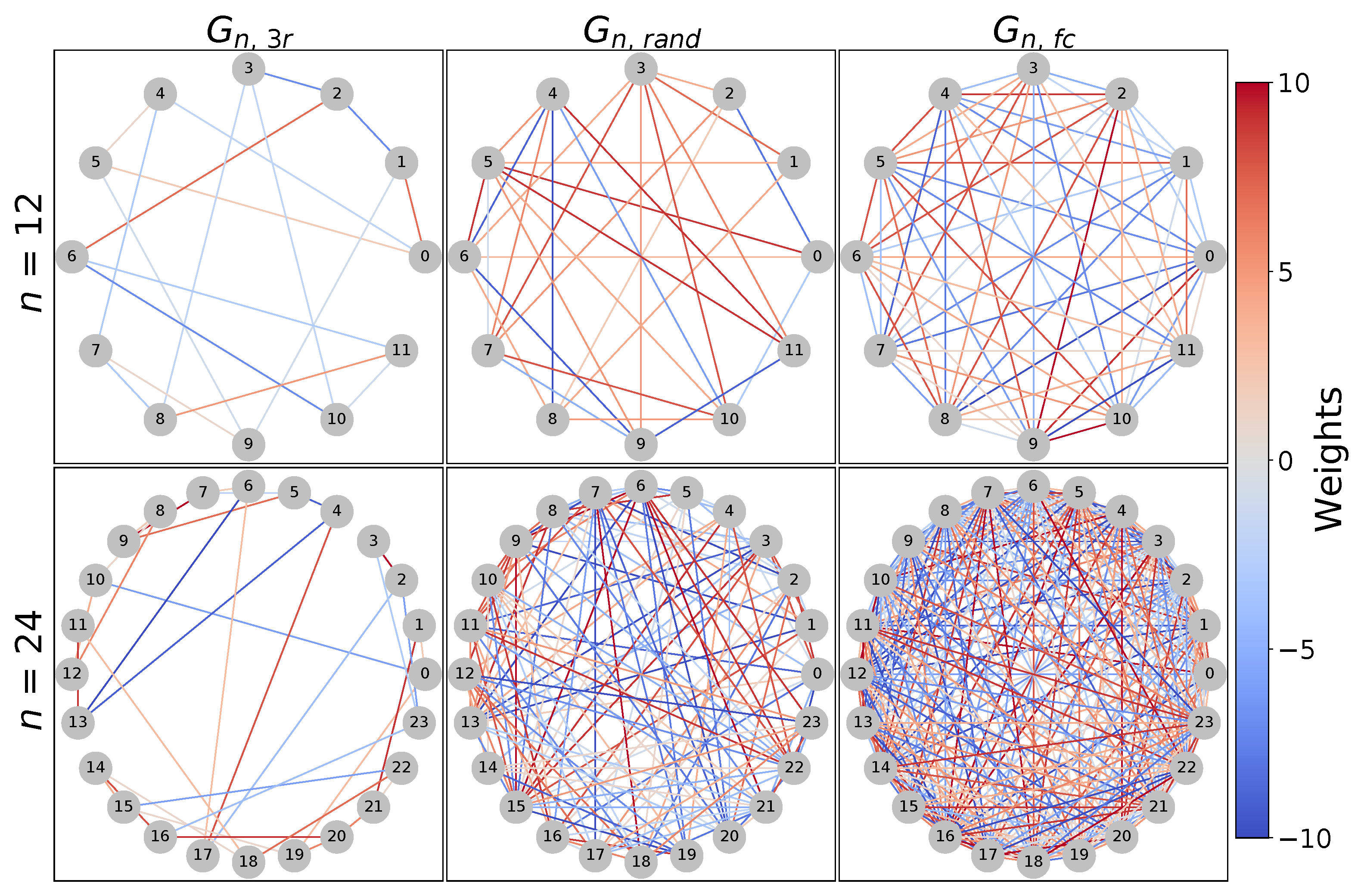
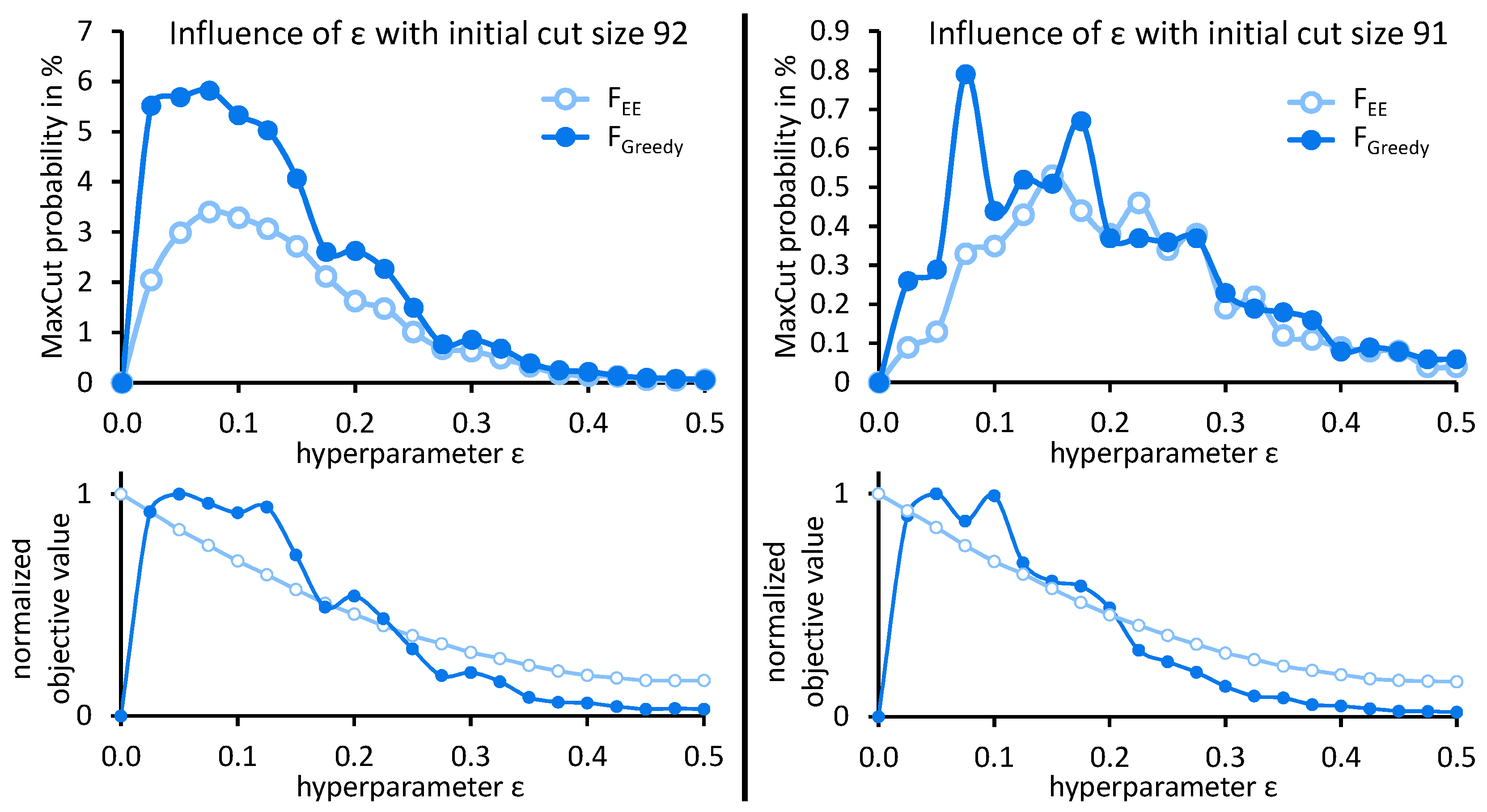
• As the input for WS-QAOA for MaxCut, we use the generated problem instances, each comprising a graph and an initial cut for this graph. For this experiment, we exemplarily focus on $G_{12,\mathit{fc}}$ as a graph with medium difficulty in our set of generated graphs (Figure 3). The problem instances for this experiment consist of this graph combined with two different initial cuts of size 91 and 92, respectively, as presented in Table 1. Both cuts are below an approximation ratio of $0.9$, thus creating problem instances for a realistic warm-starting scenario.
• For each of these problem instances, we sequentially fix the regularization parameter $\epsilon$ to each value in the range of $\{0,0.025,0.05,\dots ,0.475,0.5\}$ and execute the WS-QAOA algorithm for depth 1 (depth-1 WS-QAOA) using $F_{\mathit{EE}}$ as the objective function.
• We compute the median MaxCut probability achieved with optimized parameters from multiple replications of these executions in order to learn how the MaxCut probability correlates with $\epsilon$ for different problem instances. Multiple replications are necessary to mitigate the randomness in the measurement of quantum states.
• To determine how this correlation is influenced by the chosen objective function, steps 1 to 3 are repeated using each of the alternative objective functions given in Equations (4)–(7).
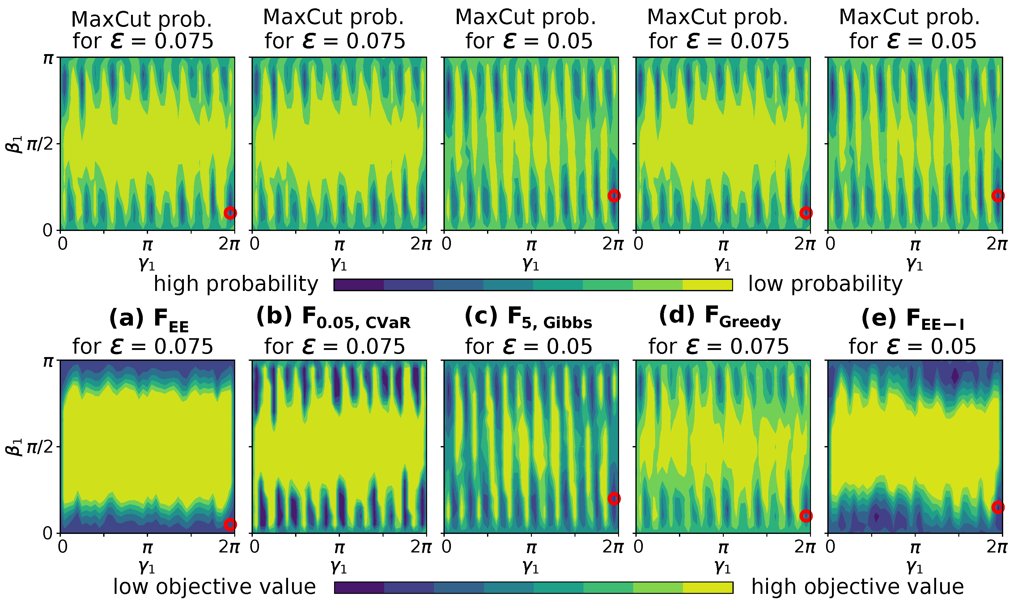
• Finally, to investigate the suitability of the objective functions for delegation of the adjustment of $\epsilon$ to the classical optimizer, we analyze the correlation of median objective values achieved in each setting with the MaxCut probability. If the $\epsilon$ values for a high MaxCut probability coincide with high objective values, the classical optimizer could be used to determine $\epsilon$ based on the objective value.

• Experiment 2: Comparison of Alternative Optimization Strategies

To compare the three optimization strategies (see Section 5.1) as formulated in RQ2 in Section 4, we proceed as follows:

• As input for WS-QAOA for MaxCut, we use a generated problem instance consisting of the graph $G_{12,\mathit{fc}}$ (Figure 3) and the initial cut of size 92 for that graph (Table 1).
• Depth-0 through depth-3 WS-QAOA are executed and optimized as prescribed by each optimization strategy. Depth-0 WS-QAOA is equivalent to merely sampling solutions from the initialized biased superposition. The regularization value $\epsilon$ is fixed to an arbitrary value for this experiment to focus on the comparison of optimization strategies for the circuit parameter optimization. $F_{\mathit{EE}}$ and $F_{\mathit{Greedy}}$ are used, exemplarily, as the objective functions.
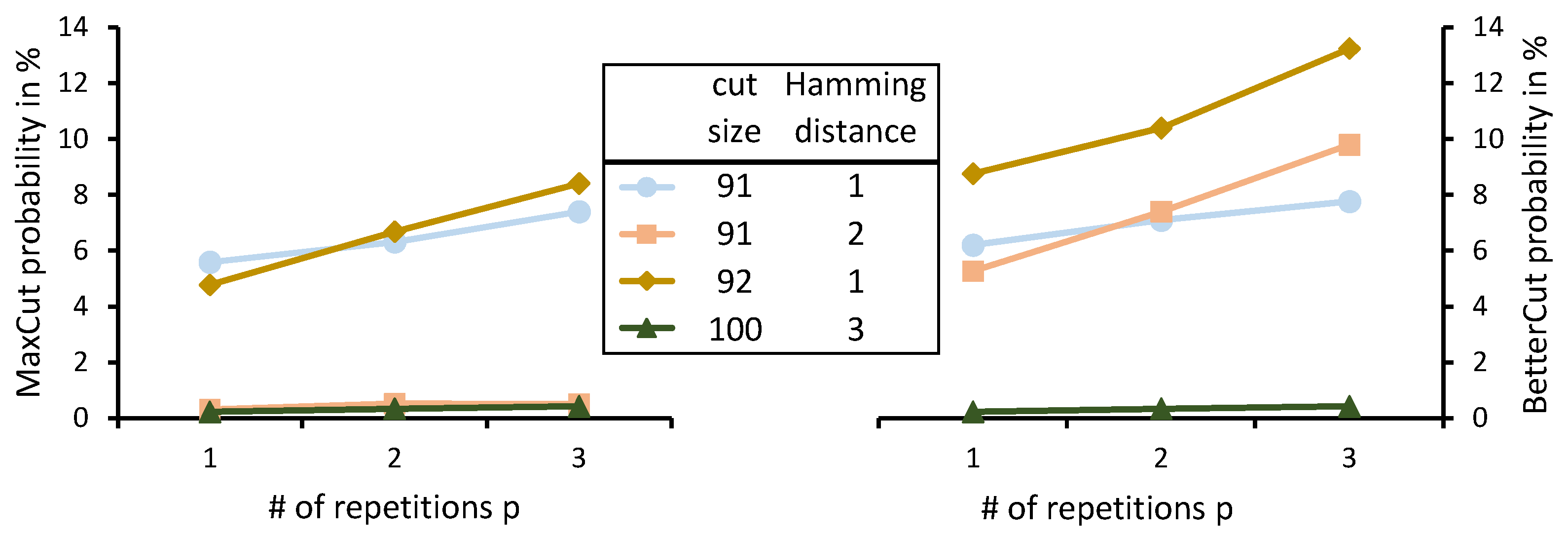
• For each depth, we record the number of epochs of the optimization loop as a platform-independent measure for execution time, i.e., the time span taken for the optimization, and the median MaxCut and BetterCut probabilities are determined using the optimized parameters from multiple replications of the optimization loop in order to assess the performance of the optimization strategies.
• Additionally, we repeat the same experiment with multiple newly generated problem instances in order to generalize the results obtained for $G_{12,\mathit{fc}}$. Therefore, we generate 20 new graphs of each kind ($G_{12,\mathit{3}\mathit{r}}$, $G_{12,\mathit{rand}}$, and $G_{12,\mathit{fc}}$) and run GW 250 times for each graph. From the resulting list of generated cuts sorted by their cut size, we select the first one of cut size below $0.9\times \mathrm{MaxCut}$ as the initial cut. For comparability between problem instances, the relative change of the MaxCut probability obtained from depth-0 to depth-1, depth-1 to depth-2, and depth-2 to depth-3 WS-QAOA is considered to assess the suitability of the optimization strategies. The optimization strategies should be able to produce an overall high MaxCut probability, that increases with the depth of the QAOA circuit, and require a low number of optimization epochs, i.e., a short execution time, which indicates high efficiency.

• Experiment 3: Evaluation of Alternative Objective Functions

To answer RQ3 formulated in Section 4, we evaluate the suitability of the five objective functions presented in Section 5.1. First, we take the same particular problem instance evaluated in Experiment 1 and Experiment 2 to evaluate and plot the objective values and MaxCut probabilities in the $({\gamma }_1,{\beta }_1)$ parameter space for the most viable regularization value $\epsilon$ for each objective function as observed in Experiment 1. We assume that the overlap is especially high for the most viable regularization value $\epsilon$, since these are the values where the minima of the objective functions found by the optimizer lead to the highest MaxCut probability. From the plots, we can then visually analyze the correlation of MaxCut probability and each objective function to assess their suitability for WS-QAOA for MaxCut.

Secondly, to compare the objective functions, we perform the following steps:

• We take generated problem instances consisting of the graphs shown in Figure 3 and corresponding initial cuts given in Table 1. For $G_{12,\mathit{fc}}$, we use the initial cut 111010111010 (cut size: 91). Thus, all initial cuts are below an approximation ratio of $0.9$ resulting in realistic warm-starting scenarios.
• We run depth-3 WS-QAOA on each graph and for each objective function. Since we focus on the different objective functions, the optimization strategy is fixed to the most suitable of the three optimization strategies from Experiment 2. Further, we employ the strategy for selecting a viable regularization value $\epsilon$ as obtained in Experiment 1.
• The median MaxCut and BetterCut probabilities from multiple replications are computed and compared to determine the suitability of objective functions with respect to the obtained solution quality.

6. Results

In this section, we present the results of our experiments described in Section 5 aimed at answering the research questions formulated in Section 4. For each experiment, we analyze the obtained results and highlight our major findings. The prototypical implementation used to obtain these results can be found on GitHub [61].

6.1. Experiment 1 Results: Influence of the Regularization Parameter $\epsilon$

Following our study design, the first question to clarify concerns the regularization parameter $\epsilon$. First, we evaluate how the MaxCut probability correlates with $\epsilon$ for the two problem instances. The results in Figure 5 indicate that the optimal regularization value $\epsilon$ (with respect to MaxCut probability) depends on the initial cut used to warm-start QAOA. For the initial cut of size 92 (Figure 5 (left)), the highest median MaxCut probability was observed at $\epsilon =0.075$ for $F_{\mathit{EE}}$. For the second initial cut of size 91 (Figure 5 (right)), the median MaxCut probability reached a maximum at $\epsilon =0.15$ for $F_{\mathit{EE}}$. Thus, a viable regularization value $\epsilon$ strongly depends on the graph at hand, since it depends on the used initial cut.

Second, we focus on how this correlation changes when we use different objective functions. As Figure 5 shows, the objective function in use also influences the MaxCut probability for different regularization values $\epsilon$. For brevity, only the results for $F_{\mathit{EE}}$ and $F_{\mathit{Greedy}}$ are compared in Figure 5. The results for the other objective functions provide similar insights and are available in the project repository on GitHub [61].

Last, to investigate the suitability of the objective functions for delegating the adjustment of $\epsilon$ to the optimizer, we compare the objective values for each regularization value $\epsilon$ with the achieved MaxCut probability in Figure 5 (bottom row). From the curves of the objective values, it is evident that the correlation between objective values and MaxCut probability is non-trivial and depends on the respective objective function. In particular, the optimal objective value for $F_{\mathit{EE}}$ is observed at $\epsilon =0$, whereas this choice for the regularization parameter $\epsilon$ yields a MaxCut probability of 0 and is thus not favorable. Whereas for $F_{\mathit{Greedy}}$, a clear correlation can be seen especially for the initial cut of size 92.

Unsurprisingly, the results of the experiments shown in Figure 5 demonstrate that finding a good regularization parameter $\epsilon$ is not trivial. Regularization values $\epsilon$ were selected to deliver a high MaxCut probability. However, since the MaxCut of a graph is not known and such exploration is not possible in general, the following two strategies for selecting the regularization value $\epsilon$ can be employed: Either selecting an arbitrary value that is expected to deliver acceptable results or letting the optimizer determine $\epsilon$. The latter requires that good objective values correlate with a high MaxCut probability. In the case of $F_{\mathit{EE}}$, as is demonstrated in Figure 5, $\epsilon$ would be optimized to 0, although the MaxCut probability for this choice of $\epsilon$ is $0\%$. Similarly, $\epsilon$ would be optimized close to 0 for $F_{\mathit{EE}-\mathit{I}}$. Therefore, such optimization is unpromising with these two objective functions.

Major observations:

• The initial cut affects the solution quality independent of the objective function. A minor change in cut size can significantly change MaxCut probabilities.
• Viable regularization values $\epsilon$ depend on the objective function in use, thus making the selection of $\epsilon$ specific to the objective function at hand.
• Classical optimizers may be usable with some objective functions to optimize the regularization parameter $\epsilon$, however, not with $F_{\mathit{EE}}$ and $F_{\mathit{EE}-\mathit{I}}$.

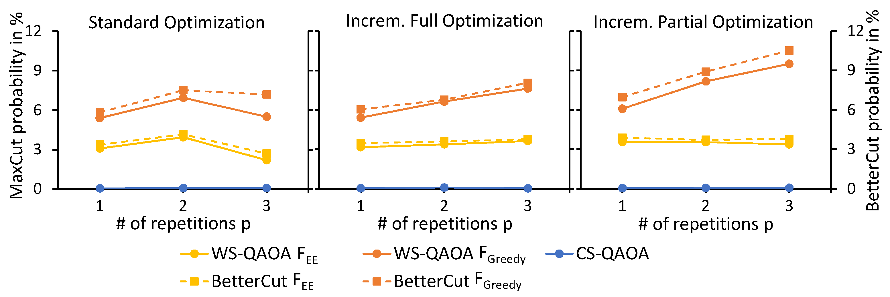
6.2. Experiment 2 Results: Comparison of Alternative Optimization Strategies

Next, we evaluate the optimization strategies following the experiment design described in Section 5.2. Figure 6 presents the results obtained with each optimization strategy for $G_{12,\mathit{fc}}$ and the initial cut of size 92 (Figure 3 and Table 1). The regularization values $\epsilon$ were adopted from searches as depicted in Figure 5. With standard optimization (Figure 6 (left)), both MaxCut and BetterCut probability drop significantly for $p=3$ repetitions of the main circuit.

This confirms our assumption that the high number of $2p$ circuit parameters, that are optimized simultaneously, makes the optimization more complex. However, the objective value was minimized to $-70.6$, $-70.9$, and $-71.7$ at $p=1,2,$ and 3, respectively (not shown in the figure). This once more illustrates an asynchronicity of the energy expectation value and the MaxCut and BetterCut probability. A slight improvement was observed using incremental full optimization (Figure 6 (center)) but for $F_{\mathit{EE}}$ both probabilities increased only marginally for $p=2$ and $p=3$. In contrast, for $F_{\mathit{Greedy}}$ consistent growth of both probabilities was observed. With incremental partial optimization (Figure 6 (right)), the probabilities observed are similar to the incremental full optimization results. Most notably, we obtained better results for higher p with both incremental optimization strategies than with standard optimization.

These results are fortified by the aggregated results of analogous experiments on multiple graphs presented in Figure 7. Both incremental full and incremental partial optimization achieved similar increase of the MaxCut probability with the depth of the QAOA circuit. However, incremental partial optimization required notably fewer epochs of COBYLA than incremental full optimization (Figure 7 (right)), since it optimizes only ${\gamma }_p,{\beta }_p$, while the other optimization strategies optimize $2p$ parameters at a time, hence, making it the most suitable of both.

Major observations:

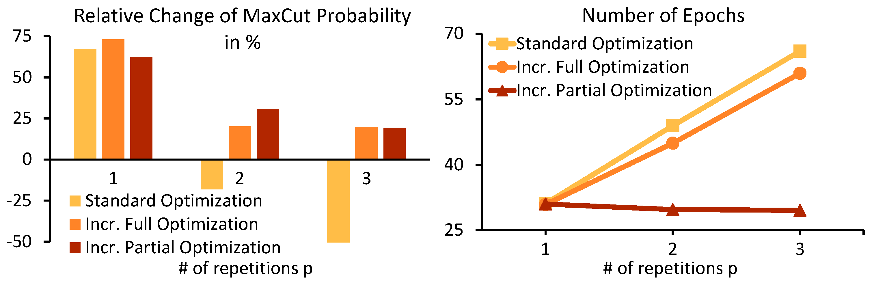
• Incremental full and incremental partial optimization lead to higher MaxCut and BetterCut probabilities than the standard optimization strategy.
• Incremental partial optimization requires less epochs of the optimizer than incremental full optimization, thus making it the least resource consuming of both incremental optimization strategies.
• Although the energy expectation objective value ($F_{\mathit{EE}}$) improves, the MaxCut and BetterCut probability may decrease at the same time, indicating a poor correlation between $F_{\mathit{EE}}$ and the solution quality.

6.3. Experiment 3 Results: Evaluation of Alternative Objective Functions

This section focuses on the comparison of the different objective functions as prescribed in Section 5.2. Therefore, we first analyze the MaxCut probabilities and objective values of each objective function in the $(\gamma ,\beta )$ parameter space before assessing the performance of each objective function for the generated problem instances. For the grid searches in the $(\gamma ,\beta )$ space, as depicted in Figure 8, the regularization parameter $\epsilon$ was set to the value that resulted in the highest median MaxCut probability for the respective problem instance in Experiment 1 (Section 6.1). In this case, these were $\epsilon =0.075$ for $F_{\mathit{EE}}$, $F_{0.05,\mathit{CVaR}}$, and $F_{\mathit{Greedy}}$ and $\epsilon =0.05$ for $F_{5,\mathit{Gibbs}}$ and $F_{\mathit{EE}-\mathit{I}}$. The results indicate that the overlap of $F_{\mathit{EE}}$ and $F_{\mathit{EE}-\mathit{I}}$ (Figure 8a,e) with the MaxCut probability at $\epsilon =0.075$ and $\epsilon =0.05$, respectively, is rather limited. Low objective values concentrate around $\beta =0$ and $\beta =\pi$, however, minima hardly coincide with the maxima for the MaxCut probability. This indicates that parameters for low objective values may not lead to high MaxCut probabilities, and, thus, optimization based on these objective functions may result in inferior solution quality. For $F_{0.05,\mathit{CVaR}}$, $F_{5,\mathit{Gibbs}}$ and $F_{\mathit{Greedy}}$ (Figure 8b–d), the overlap is much more obvious, which indicates that optimization based on these objective functions may result in higher solution quality. Note that $\alpha =0.05$ for $F_{0.05,\mathit{CVaR}}$ implies a lower bound for the minimum objective value that is reached each time when the MaxCut probability is higher than $5\%$. This effect visibly widens the minima of the objective function in Figure 8.

Minima for $F_{0.05,\mathit{CVaR}}$ are not marked in Figure 8b, since too many points take the same minimal value.

We now proceed with the evaluation of the performance of each objective function for each of the problem instances as prescribed in Section 5.2. Both options for selecting the regularization parameter $\epsilon$ that we inferred in Section 6.1 are compared. First, we fixed the regularization parameter $\epsilon$ to an arbitrary value that we expected to be a generally acceptable choice. The results obtained with this strategy are presented in

Table 2. (Left): Final MaxCut and BetterCut probabilities after depth-3 WS-QAOA with fixed regularization value $\epsilon$. Problem instances consisting of each graph G in Figure 3 and each objective function F (Equations (3)–(7)) were used. $\alpha$ was fixed at $0.05$. $\eta$ was set to 5 for the 12-node graphs and 2 for the 24-node graphs. The smaller $\eta$ accounts for larger achievable cut sizes in the 24-node graphs; however, the values are, in essence, arbitrary (see [34]). Initial cuts are given in Table 1, for $G_{12,\mathit{fc}}$ the initial cut was 111010111010 (cut size: 91). Values reflect median probabilities observed in 20 runs per configuration. (Right): Final probabilities after depth-3 WS-QAOA when $\epsilon$ is determined by the optimizer during the depth-1 round of incremental partial optimization. The same problem instances as above and the objective functions $F_{\alpha ,\mathit{CVaR}}$, $F_{\eta ,\mathit{Gibbs}}$, and $F_{\mathit{Greedy}}$ are considered. Highest values in each row are highlighted.

	Final MaxCut probabilities after depth-3 WS-QAOA
	with fixed regularization value $\epsilon =0.125$						with optimized regularization value $\epsilon$
	F	$F_{\mathit{EE}}$	$F_{\alpha ,\mathit{CVaR}}$	$F_{\eta ,\mathit{Gibbs}}$	$F_{\mathit{Greedy}}$	$F_{\mathit{EE}-\mathit{I}}$	$F_{\mathit{EE}}$	$F_{\alpha ,\mathit{CVaR}}$	$F_{\eta ,\mathit{Gibbs}}$	$F_{\mathit{Greedy}}$	$F_{\mathit{EE}-\mathit{I}}$
G
$G_{12,\mathit{3}\mathit{r}}$		0.13%	0.26%	0.38%	0.20%	0.11%	-	0.06%	0.34%	0.14%	-
$G_{12,\mathit{rand}}$		0.00%	0.02%	0.17%	0.02%	0.00%	-	0.01%	0.28%	0.02%	-
$G_{12,\mathit{fc}}$		0.37%	1.00%	2.03%	0.60%	0.54%	-	0.63%	1.74%	0.49%	-
$G_{24,\mathit{3}\mathit{r}}$		0.03%	0.02%	0.04%	0.00%	0.00%	-	0.00%	0.00%	0.03%	-
$G_{24,\mathit{rand}}$		0.00%	0.00%	0.00%	0.00%	0.00%	-	0.00%	0.00%	0.00%	-
$G_{24,\mathit{fc}}$		0.08%	0.08%	0.16%	0.08%	0.08%	-	0.00%	0.15%	0.17%	-
		Final BetterCut probabilities after depth-3 WS-QAOA
		with fixed regularization value $\epsilon =0.125$					with optimized regularization value $\epsilon$
	F	$F_{\mathit{EE}}$	$F_{\alpha ,\mathit{CVaR}}$	$F_{\eta ,\mathit{Gibbs}}$	$F_{\mathit{Greedy}}$	$F_{\mathit{EE}-\mathit{I}}$	$F_{\mathit{EE}}$	$F_{\alpha ,\mathit{CVaR}}$	$F_{\eta ,\mathit{Gibbs}}$	$F_{\mathit{Greedy}}$	$F_{\mathit{EE}-\mathit{I}}$
G
$G_{12,\mathit{3}\mathit{r}}$		4.54%	6.46%	5.20%	9.11%	6.34%	-	5.92%	2.70%	12.32%	-
$G_{12,\mathit{rand}}$		1.28%	3.87%	0.70%	3.00%	1.89%	-	2.67%	0.69%	3.20%	-
$G_{12,\mathit{fc}}$		6.48%	8.53%	5.17%	10.69%	9.00%	-	9.03%	5.33%	14.13%	-
$G_{24,\mathit{3}\mathit{r}}$		4.23%	4.04%	3.01%	4.59%	3.56%	-	0.00%	2.02%	11.59%	-
$G_{24,\mathit{rand}}$		1.13%	1.78%	1.48%	1.62%	1.20%	-	0.00%	5.89%	5.56%	-
$G_{24,\mathit{fc}}$		2.36%	2.82%	1.63%	2.98%	2.51%	-	0.00%	3.02%	9.40%	-

(left). Moreover, $\alpha$ for $F_{\alpha ,\mathit{CVaR}}$ and $\eta$ for $F_{\eta ,\mathit{Gibbs}}$ were fixed at arbitrary values, as choosing them is likewise challenging and out of the scope of this paper. The results show that the median MaxCut probability obtained for the 24-node graphs is significantly lower than that for the 12-node graphs. Particularly, for $G_{24,\mathit{rand}}$ the MaxCut was not found at all in any run for any of the objective functions and QAOA-depths. The MaxCut of $G_{12,\mathit{rand}}$ was found only by optimizing $F_{\alpha ,\mathit{CVaR}}$, $F_{5,\mathit{Gibbs}}$, and $F_{\mathit{Greedy}}$. But the median probability was significantly lower than for the other two 12-node graphs. Table 2 (bottom left-hand side) shows, that the median BetterCut probabilities achieved for the 24-node graphs were mostly lower than for the 12-node graphs.

For the second option for selecting the regularization value $\epsilon$, we repeated the same experiments, but this time the regularization parameter $\epsilon$ was determined by COBYLA during the depth-1 round of the incremental partial optimization. The optimization of $\epsilon$ was constrained to the range $[0,0.5]$. The final MaxCut and BetterCut probabilities for these experiments are presented in Table 2 (right). As expected, $\epsilon$ was optimized close to 0 for $F_{\mathit{EE}}$ and $F_{\mathit{EE}-\mathit{I}}$, resulting in negligible MaxCut and BetterCut probabilities (therefore not shown in Table 2 (right), see project repository [61]). The optimization of $\epsilon$ for $F_{\alpha ,\mathit{CVaR}}$ resulted in decreased MaxCut probabilities, while BetterCut probabilities decreased for most graph instances. Most notably, $\epsilon$ was optimized to 0 for all 24-node graphs, resulting in both MaxCut and BetterCut probabilities reduced to $0\%$. For the 12-node graphs, $F_{\mathit{Greedy}}$ and $F_{\eta ,\mathit{Gibbs}}$ produced mostly similar MaxCut and BetterCut probabilities compared to the experiments with the fixed regularization value $\epsilon$. For the 24-node graphs on the other hand, the optimization of $\epsilon$ with $F_{\mathit{Greedy}}$ resulted in significantly increased BetterCut probabilities. Moreover, the MaxCut probability for $G_{24,\mathit{fc}}$ increased with $F_{\mathit{Greedy}}$. In these cases, $\epsilon$ was optimized to values around $0.025$ to $0.085$, which differs clearly from the fixed value of $0.125$. Evidently, the optimized $\epsilon$ were more suitable in these cases, which shows that hyperparameter optimization is a viable approach when a compatible objective function is used.

When $\epsilon$ was optimized in each round of the incremental partial optimization instead, i.e., at depth 1 through 3, the resulting probabilities were significantly lower, although the optimized $\epsilon$ were similar to those in the experiments described above. Similar to the experiments in Section 6.2, it appears that more optimized parameters led to more optimization epochs and inferior results. Notably, the optimized $\epsilon$ values at each depth did not differ significantly from each other, which supports the assumption that $\epsilon$ is independent of $p\in \{1,2,3\}$.

Major observations:

• The overlap of MaxCut probability and objective values is poorer for $F_{\mathit{EE}}$ and $F_{\mathit{EE}-\mathit{I}}$ than for other objective functions, which consequently led to increased MaxCut probabilities compared to $F_{\mathit{EE}}$ and $F_{\mathit{EE}-\mathit{I}}$. Therefore, these alternative objective functions should be preferred for WS-QAOA over the standard energy expectation objective function $F_{\mathit{EE}}$.
• In our setup, $F_{\eta ,\mathit{Gibbs}}$ resulted in the highest MaxCut probabilities, while $F_{\mathit{Greedy}}$ resulted in the highest BetterCut probabilities.
• When the regularization parameter $\epsilon$ is determined by the optimizer, the performance of $F_{\eta ,\mathit{Gibbs}}$ and $F_{\mathit{Greedy}}$ with respect to MaxCut and BetterCut probability, respectively, can increase significantly compared to the fixed value for $\epsilon$.

7. Discussion

In this section, we discuss further and summarize the results of the experiments presented in Section 6 to provide a more comprehensive view of the hyperparameter selection aspects formulated in our research questions.

7.1. Choice of the Regularization Parameter $\epsilon$

The results of Experiment 1 (see Section 6.1) and Experiment 3 (see Section 6.3) show that the regularization parameter $\epsilon$ depends on both (i) the problem instance at hand and (ii) the objective function employed during the optimization. Regularization values $\epsilon$ that lead to a high solution quality with one objective function on a particular problem instance may result in low solution quality when the objective function is changed, e.g., as seen with the problem instance considered in Figure 5 (right), where the regularization value leading to the highest solution quality when objective function $F_{\mathit{Greedy}}$ is employed, results in a poor solution quality when $F_{\mathit{EE}}$ is used instead. Based on the conducted experiments, we identified two possible strategies for choosing the regularization parameter $\epsilon$:

• A naïve strategy is to fix the regularization parameter $\epsilon$ to an arbitrary value, thus accepting some loss of solution quality due to sub-optimality for particular combinations of problem instances and objective function. The benefit of this strategy is its simplicity, and the results of Experiment 3 suggest it can produce acceptable solutions.
• As an alternative strategy, selecting the regularization parameter $\epsilon$ can be delegated to a classical optimizer. However, this requires a suitable objective function. As shown in Experiment 3, the objective functions $F_{\eta ,\mathit{Gibbs}}$ and $F_{\mathit{Greedy}}$ are compatible with this strategy. The benefit of this strategy is that it can potentially determine the optimal regularization value $\epsilon$ for a problem instance automatically and thus achieve a better solution quality compared to setting an arbitrary value. However, it introduces additional optimization difficulty that may lead to increased execution time of the optimization process.

Clearly, the naïve strategy could potentially be improved by heuristically determining generally acceptable values for categories of problem instances in combination with a specific objective function, thus improving the solution quality obtained with the strategy. Moreover, the alternative strategy relying on objective functions compatible with the optimization of $\epsilon$ could likewise profit from such heuristic values used as a starting point for the classical optimization of $\epsilon$ to speed up the process and reduce additional optimization effort.

7.2. Choice of the Optimization Strategy

From the results of Experiment 2 (see Section 6.2), it can be observed that alternative optimization strategies can significantly increase the solution quality. The presented alternative incremental optimization strategies essentially execute lower-depth WS-QAOA instances to obtain initial parameter values for higher-depth WS-QAOA circuit parameters (in the case of incremental full optimization) or fix some parameters (in the case of incremental partial optimization). This results in the execution of multiple optimization loops for different depths of WS-QAOA, which increases the total number of optimization epochs. However, when the incremental partial optimization strategy was employed, the total number of epochs was similar to that used for the standard optimization approach. Therefore, one important recommendation derived based on our experimental results is to choose the incremental partial optimization strategy over the other employed optimization strategies. More specifically, the incremental partial optimization strategy (i) performs similarly well with respect to solution quality compared to the incremental full optimization strategy and (ii) its execution time is similar to the standard optimization strategy.

7.3. Choice of the Objective Function

The results of our experiments also provide some insights into different objective functions and the corresponding solution quality achieved with each. Of all objective functions, we learned most about the correlation of the energy expectation objective function $F_{\mathit{EE}}$ with the MaxCut probability and thus its suitability for WS-QAOA for MaxCut. In Experiment 1 (see Section 6.1) and Experiment 3 (see Section 6.3), $F_{\mathit{EE}}$ leads to the lowest MaxCut probabilities compared to $F_{\alpha ,\mathit{CVaR}}$, $F_{\eta ,\mathit{Gibbs}}$, and $F_{\mathit{Greedy}}$, while the results obtained with $F_{\mathit{EE}-\mathit{I}}$ were similar. However, $F_{\mathit{EE}-\mathit{I}}$ resulted in significantly higher BetterCuts probabilities for some problem instances in Experiment 3 (Table 2 (bottom left-hand side)). Furthermore, we observed in Experiment 2 (see Section 6.2) that objective values increased with the number of repetitions of the QAOA ansatz ($p\in \{1,2,3\}$) when $F_{\mathit{EE}}$ was employed, but the achieved MaxCut probability stagnated or decreased, particularly with standard optimization. The results from Experiment 3 made clear, that this is due to insufficient correlation between MaxCut probability and the objective function in the parameter space, where the minima of $F_{\mathit{EE}}$ and the MaxCut probability did not match. Thus, the optimizer finds parameter values that lead to a high objective value, but not necessarily to a high MaxCut probability. Eventually, this also leads to the overall comparatively poor performance of $F_{\mathit{EE}}$. This also occurred in the second half of Experiment 3, where we ran WS-QAOA on our sample problem instances with different objective functions.

These results lead to an important observation. Using an alternative objective function when executing WS-QAOA for MaxCut can result in significantly better solution quality than the standard objective function $F_{\mathit{EE}}$. More specifically, our experiments showed that the objective functions $F_{\alpha ,\mathit{CVaR}}$, $F_{\eta ,\mathit{Gibbs}}$, and $F_{\mathit{Greedy}}$ are more preferable with $F_{\eta ,\mathit{Gibbs}}$ performing best with respect to MaxCut probabilities and $F_{\mathit{Greedy}}$ with respect to BetterCut probabilities in Experiment 3. Moreover, the latter two are also compatible with optimizing the regularization parameter $\epsilon$ as elaborated in Section 7.1, thus enabling the additional improvement of the solution quality. A clear advantage of $F_{\mathit{Greedy}}$, that was introduced in this work specifically for WS-QAOA for MaxCut, is that it does not come with additional hyperparameters, but instead takes the initial cut of the problem instances into account. Thus, it avoids adding to the overall problem of hyperparameter selection.

7.4. Influence of Hamming Distance on Solution Quality

In Experiment 1 (see Section 6.1), we observed that the MaxCut probability obtained with the initial cut of size 92 was significantly higher in general than that obtained with the initial cut of size 91. On closer examination of these initial cuts, it can be observed that the Hamming distance between the MaxCut and the initial cut of size 92 is 1 and, thus, lower than the Hamming distance of 2 between the MaxCut and initial cut of size 91. The Hamming distance is the number of positions where the bit strings of two cuts have different values [62].

These observations led to a suspicion that the Hamming distance of an initial cut to MaxCuts correlates with the solution quality achieved in WS-QAOA. Further analysis of the initial cuts used in Experiment 3 (see Section 5.2) revealed that the Hamming distances of the initial cuts for $G_{12,\mathit{3}\mathit{r}}$, $G_{12,\mathit{rand}}$, and $G_{12,\mathit{fc}}$ were 3, 5, and 2, respectively. For $G_{24,\mathit{3}\mathit{r}}$, $G_{24,\mathit{rand}}$, and $G_{24,\mathit{fc}}$ the distances were 2, 6, and 3. Interestingly, the MaxCut and BetterCut probabilities were generally higher for those problem instances where the Hamming distance was low, and vice versa. To further examine the influence of the initial cut’s Hamming distance and cut size on the solution quality of WS-QAOA, we compared 4 different initial cuts for $G_{12,\mathit{fc}}$. The results shown in Figure 9 support our assumption regarding the correlation between the Hamming distance and the achieved solution quality. For example, of two different initial cuts with the same cut size of 91, the cut with the smaller Hamming distance led to a significantly higher MaxCut probability.

Generally, the MaxCut probability seems to depend on a cut’s Hamming distance to the MaxCut rather than its cut size. For example, the largest initial cut of size 100 led to the lowest MaxCut probabilities in this comparison, presumably due to its high Hamming distance to the MaxCut. The results also show that the BetterCut probability decreases with the cut size since the remaining number of cuts better than the initial cut decreases with its size. Particularly, for the initial cut of size 100, the MaxCut probability and BetterCut probability are identical since no cuts larger than 100 exist except the MaxCut.

8. Conclusions and Future Work

Hyperparameter selection for QML algorithms is challenging, especially for hyperparameters specific to the quantum domain. In this work, we experimented with three important hyperparameters of a WS-QAOA for the MaxCut problem. For the regularization parameter, $\epsilon$, of WS-QAOA, which tunes the bias of the algorithm to a classically pre-computed solution, hyperparameter optimization using a classical optimizer proved successful in cases where a suitable objective function was employed. Of the two alternative optimization strategies that we assessed for the classical optimization of the WS-QAOA circuit parameters, incremental partial optimization, i.e., a layer-wise optimization strategy that successively optimizes two of the circuit parameters in each step, performed best considering that it resulted in significantly increased solution quality but required only a few more optimization epochs than the standard optimization approach. In our experiments, we considered four alternatives to the standard energy expectation objective function for the optimization process. All of these alternatives performed at least as well as the standard objective function with respect to the resulting solution quality. Particularly, two of the alternative objective functions proved suitable for the classical optimization of the regularization parameter $\epsilon$ while producing the best results with respect to improving upon the pre-computed classical result and producing an optimal solution, respectively. We believe that these results will aid further experiments with and applications of WS-QAOA, as well as in other optimization problems, as they not only demonstrate the importance of quantum-specific hyperparameters, but also deepen the understanding of approaches to cope with parameter selection.

We see manifold research opportunities related to WS-QAOA and hyperparameter selection for the algorithm. Regarding alternative objective functions, there is clearly potential to construct more such functions, e.g., by the combination of the different existing concepts. For example, some objective functions are vulnerable for barren plateaus that increase the optimization difficulty. These barren plateaus could be detected and replaced by values generated with another objective function to help direct the optimization. The incremental optimization strategies presented in this work, could also be developed further. Instead of moving sequentially from one WS-QAOA depth to the next and reusing the optimized circuit parameters as initial (or fixed) values for the next iteration, lower-depth WS-QAOA could well be executed multiple times to receive better parameter values. For example, from optimized parameters of 10 replications of depth-1 WS-QAOA, the best-performing parameters could be passed to the depth-2 WS-QAOA step, which may increase the chances of finding a global optimum. Another idea is relying on WS-QAOA to find a cut better than the classically computed initial cut and then running another WS-QAOA instance using this improved solution with the aim of progressing hand over hand to an optimal solution. An important point that is already scratched with the incremental optimization strategies is determining initial parameters for WS-QAOA circuits. We are aware of works concerning the transferability of QAOA parameters between different problem instances or classical pre-computation of QAOA circuit parameters. In future work, we plan to focus on such concepts and combine them with WS-QAOA to speed up the classical parameter optimization. Moreover, the practical relevancy of our observation regarding the initial cut’s Hamming distance to a MaxCut remains an open question to examine. Although this correlation cannot be of direct help since computing the Hamming distance requires solving the MaxCut problem in the first place, being aware of it deepens the understanding of the WS-QAOA algorithm and may indeed help improving it. First intuition might be bringing multiple initial cuts in superposition so as to increase the chance that at least one of them is close to a MaxCut. Further, we plan on transferring and rerunning our experiments on different quantum devices and with larger problem instances to derive more precise guidelines for hyperparameter selection and assist in proceeding towards real quantum devices and their applications for real-world use cases.

References

1. Cao, Y.; Romero, J.; Olson, J.P.; Degroote, M.; Johnson, P.D.; Kieferová, M.; Kivlichan, I.D.; Menke, T.; Peropadre, B.; Sawaya, N.P.D.; et al. Quantum Chemistry in the Age of Quantum Computing. Chem. Rev. 2019, 119, 10856–10915. [Google Scholar] [CrossRef] [PubMed] [Green Version]
2. DeBenedictis, E.P. A Future with Quantum Machine Learning. Computer 2018, 51, 68–71. [Google Scholar] [CrossRef]
3. Schuld, M.; Sinayskiy, I.; Petruccione, F. An introduction to quantum machine learning. Contemp. Phys. 2015, 56, 172–185. [Google Scholar] [CrossRef] [Green Version]
4. Biamonte, J.; Wittek, P.; Pancotti, N.; Rebentrost, P.; Wiebe, N.; Lloyd, S. Quantum machine learning. Nature 2017, 549, 195–202. [Google Scholar] [CrossRef]
5. Arunachalam, S.; de Wolf, R. Guest Column: A Survey of Quantum Learning Theory. SIGACT News 2017, 48, 41–67. [Google Scholar] [CrossRef]
6. Khan, T.M.; Robles-Kelly, A. Machine Learning: Quantum vs Classical. IEEE Access 2020, 8, 219275–219294. [Google Scholar] [CrossRef]
7. Huang, H.L.; Du, Y.; Gong, M.; Zhao, Y.; Wu, Y.; Wang, C.; Li, S.; Liang, F.; Lin, J.; Xu, Y.; et al. Experimental quantum generative adversarial networks for image generation. Phys. Rev. Appl. 2021, 16, 024051. [Google Scholar] [CrossRef]
8. Havlíček, V.; Córcoles, A.D.; Temme, K.; Harrow, A.W.; Kandala, A.; Chow, J.M.; Gambetta, J.M. Supervised learning with quantum-enhanced feature spaces. Nature 2019, 567, 209–212. [Google Scholar] [CrossRef] [Green Version]
9. Zahedinejad, E.; Zaribafiyan, A. Combinatorial optimization on gate model quantum computers: A survey. arXiv 2017, arXiv:1708.05294. [Google Scholar]
10. Harrigan, M.P.; Sung, K.J.; Neeley, M.; Satzinger, K.J.; Arute, F.; Arya, K.; Atalaya, J.; Bardin, J.C.; Barends, R.; Boixo, S.; et al. Quantum approximate optimization of non-planar graph problems on a planar superconducting processor. Nat. Phys. 2021, 17, 332–336. [Google Scholar] [CrossRef]
11. Huang, H.L.; Wu, D.; Fan, D.; Zhu, X. Superconducting quantum computing: A review. Sci. China Inf. Sci. 2020, 63, 1–32. [Google Scholar] [CrossRef]
12. Krantz, P.; Kjaergaard, M.; Yan, F.; Orlando, T.P.; Gustavsson, S.; Oliver, W.D. A quantum engineer’s guide to superconducting qubits. Appl. Phys. Rev. 2019, 6, 021318. [Google Scholar] [CrossRef]
13. Bruzewicz, C.D.; Chiaverini, J.; McConnell, R.; Sage, J.M. Trapped-ion quantum computing: Progress and challenges. Appl. Phys. Rev. 2019, 6, 021314. [Google Scholar] [CrossRef] [Green Version]
14. Blatt, R.; Roos, C.F. Quantum simulations with trapped ions. Nat. Phys. 2012, 8, 277–284. [Google Scholar] [CrossRef]
15. Preskill, J. Quantum computing in the NISQ era and beyond. Quantum 2018, 2, 79. [Google Scholar] [CrossRef]
16. Leymann, F.; Barzen, J. The bitter truth about gate-based quantum algorithms in the NISQ era. Quantum Sci. Technol. 2020, 5, 044007. [Google Scholar] [CrossRef]
17. Farhi, E.; Goldstone, J.; Gutmann, S. A quantum approximate optimization algorithm. arXiv 2014, arXiv:1411.4028. [Google Scholar]
18. Cerezo, M.; Arrasmith, A.; Babbush, R.; Benjamin, S.C.; Endo, S.; Fujii, K.; McClean, J.R.; Mitarai, K.; Yuan, X.; Cincio, L.; et al. Variational Quantum Algorithms. arXiv 2020, arXiv:2012.09265. [Google Scholar] [CrossRef]
19. Yildirim, E.A.; Wright, S.J. Warm-start strategies in interior-point methods for linear programming. SIAM J. Optim. 2002, 12, 782–810. [Google Scholar] [CrossRef]
20. Ralphs, T.; Güzelsoy, M. Duality and warm starting in integer programming. In Proceedings of the 2006 NSF Design, Service, and Manufacturing Grantees and Research Conference, St. Louis, MO, USA, 24–27 July 2006. [Google Scholar]
21. John, E.; Yıldırım, E.A. Implementation of warm-start strategies in interior-point methods for linear programming in fixed dimension. Comput. Optim. Appl. 2008, 41, 151–183. [Google Scholar] [CrossRef]
22. Shahzad, A.; Kerrigan, E.C.; Constantinides, G.A. A warm-start interior-point method for predictive control. In Proceedings of the UKACC International Conference on CONTROL 2010, Coventry, UK, 7–10 September 2010. [Google Scholar]
23. Poloczek, M.; Wang, J.; Frazier, P.I. Warm starting Bayesian optimization. In Proceedings of the 2016 Winter Simulation Conference (WSC), Washington, DC, USA, 11–14 December 2016; pp. 770–781. [Google Scholar]
24. Bertsimas, D.; King, A.; Mazumder, R. Best subset selection via a modern optimization lens. Ann. Stat. 2016, 44, 813–852. [Google Scholar] [CrossRef] [Green Version]
25. Feurer, M.; Letham, B.; Bakshy, E. Scalable meta-learning for Bayesian optimization. Stat 2018, 1050, 6. [Google Scholar]
26. Weigold, M.; Barzen, J.; Leymann, F.; Vietz, D. Patterns for Hybrid Quantum Algorithms. In Proceedings of the Symposium and Summer School on Service-Oriented Computing, Virtual Event, 13–17 September 2021; Springer: Cham, Switzerland, 2021; pp. 34–51. [Google Scholar]
27. Egger, D.J.; Mareček, J.; Woerner, S. Warm-starting quantum optimization. Quantum 2021, 5, 479. [Google Scholar] [CrossRef]
28. Tate, R.; Farhadi, M.; Herold, C.; Mohler, G.; Gupta, S. Bridging Classical and Quantum with SDP initialized warm-starts for QAOA. arXiv 2020, arXiv:2010.14021. [Google Scholar]
29. Goemans, M.X.; Williamson, D.P. Improved approximation algorithms for maximum cut and satisfiability problems using semidefinite programming. J. ACM (JACM) 1995, 42, 1115–1145. [Google Scholar] [CrossRef]
30. Barkoutsos, P.K.; Nannicini, G.; Robert, A.; Tavernelli, I.; Woerner, S. Improving Variational Quantum Optimization using CVaR. Quantum 2020, 4, 256. [Google Scholar] [CrossRef]
31. Beaulieu, D.; Pham, A. Max-cut Clustering Utilizing Warm-Start QAOA and IBM Runtime. arXiv 2021, arXiv:2108.13464. [Google Scholar]
32. Beaulieu, D.; Pham, A. Evaluating performance of hybrid quantum optimization algorithms for MAXCUT Clustering using IBM runtime environment. arXiv 2021, arXiv:2112.03199. [Google Scholar]
33. Tate, R.; Gard, B.; Mohler, G.; Gupta, S. Classically-inspired Mixers for QAOA Beat Goemans-Williamson’s Max-Cut at Low Circuit Depths. arXiv 2021, arXiv:2112.11354. [Google Scholar]
34. Li, L.; Fan, M.; Coram, M.; Riley, P.; Leichenauer, S. Quantum optimization with a novel Gibbs objective function and ansatz architecture search. Phys. Rev. Res. 2020, 2, 023074. [Google Scholar] [CrossRef] [Green Version]
35. Kolotouros, I.; Wallden, P. An evolving objective function for improved variational quantum optimisation. arXiv 2021, arXiv:2105.11766. [Google Scholar]
36. Carolan, J.; Mohseni, M.; Olson, J.P.; Prabhu, M.; Chen, C.; Bunandar, D.; Niu, M.Y.; Harris, N.C.; Wong, F.N.; Hochberg, M.; et al. Variational quantum unsampling on a quantum photonic processor. Nat. Phys. 2020, 16, 322–327. [Google Scholar] [CrossRef] [Green Version]
37. Skolik, A.; McClean, J.R.; Mohseni, M.; van der Smagt, P.; Leib, M. Layerwise learning for quantum neural networks. Quantum Mach. Intell. 2021, 3, 1–11. [Google Scholar] [CrossRef]
38. Sim, S.; Romero, J.; Gonthier, J.F.; Kunitsa, A.A. Adaptive pruning-based optimization of parameterized quantum circuits. Quantum Sci. Technol. 2021, 6, 025019. [Google Scholar] [CrossRef]
39. Lyu, C.; Montenegro, V.; Bayat, A. Accelerated variational algorithms for digital quantum simulation of many-body ground states. Quantum 2020, 4, 324. [Google Scholar] [CrossRef]
40. Campos, E.; Nasrallah, A.; Biamonte, J. Abrupt transitions in variational quantum circuit training. Phys. Rev. A 2021, 103, 032607. [Google Scholar] [CrossRef]
41. Campos, E.; Rabinovich, D.; Akshay, V.; Biamonte, J. Training Saturation in Layerwise Quantum Approximate Optimisation. arXiv 2021, arXiv:2106.13814. [Google Scholar]
42. Salm, M.; Barzen, J.; Leymann, F.; Weder, B. About a Criterion of Successfully Executing a Circuit in the NISQ Era: What wd≪1/ϵeff Really Means. In Proceedings of the 1st ACM SIGSOFT International Workshop on Architectures and Paradigms for Engineering Quantum Software (APEQS 2020), Virtual, 13 November 2020; ACM: New York, NY, USA, 2020; pp. 10–13. [Google Scholar] [CrossRef]
43. Leymann, F.; Barzen, J.; Falkenthal, M.; Vietz, D.; Weder, B.; Wild, K. Quantum in the Cloud: Application Potentials and Research Opportunities. In Proceedings of the 10th International Conference on Cloud Computing and Service Science (CLOSER 2020), Prague, Czech Republic, 7–9 May 2020; SciTePress: Setúbal, Portugal, 2020; pp. 9–24. [Google Scholar]
44. Farhi, E.; Goldstone, J.; Gutmann, S.; Sipser, M. Quantum Computation by Adiabatic Evolution. arXiv 2000, arXiv:0001106. [Google Scholar]
45. Dalzell, A.M.; Harrow, A.W.; Koh, D.E.; Placa, R.L.L. How many qubits are needed for quantum computational supremacy? arXiv 2018, arXiv:1805.05224v3. [Google Scholar] [CrossRef]
46. Akshay, V.; Philathong, H.; Zacharov, I.; Biamonte, J. Reachability Deficits in Quantum Approximate Optimization of Graph Problems. arXiv 2020, arXiv:2007.09148v2. [Google Scholar] [CrossRef]
47. Majumdar, R.; Madan, D.; Bhoumik, D.; Vinayagamurthy, D.; Raghunathan, S.; Sur-Kolay, S. Optimizing Ansatz Design in QAOA for Max-cut. arXiv 2021, arXiv:2106.02812. [Google Scholar]
48. Karp, R.M. Reducibility among combinatorial problems. In Complexity of Computer Computations; Springer: Boston, MA, USA, 1972; pp. 85–103. [Google Scholar]
49. Khot, S.; Kindler, G.; Mossel, E.; O’Donnell, R. Optimal inapproximability results for MAX-CUT and other 2-variable CSPs? SIAM J. Comput. 2007, 37, 319–357. [Google Scholar] [CrossRef] [Green Version]
50. Håstad, J. Some optimal inapproximability results. J. ACM (JACM) 2001, 48, 798–859. [Google Scholar] [CrossRef]
51. Barahona, F.; Grötschel, M.; Jünger, M.; Reinelt, G. An application of combinatorial optimization to statistical physics and circuit layout design. Oper. Res. 1988, 36, 493–513. [Google Scholar] [CrossRef] [Green Version]
52. Ding, C.H.; He, X.; Zha, H.; Gu, M.; Simon, H.D. A min-max cut algorithm for graph partitioning and data clustering. In Proceedings of the 2001 IEEE International Conference on Data Mining, San Jose, CA, USA, 29 November–2 December 2001; pp. 107–114. [Google Scholar]
53. Barzen, J. From Digital Humanities to Quantum Humanities: Potentials and Applications. arXiv 2021, arXiv:2103.11825. [Google Scholar]
54. Yang, L.; Shami, A. On hyperparameter optimization of machine learning algorithms: Theory and practice. Neurocomputing 2020, 415, 295–316. [Google Scholar] [CrossRef]
55. Claesen, M.; Moor, B.D. Hyperparameter Search in Machine Learning. arXiv 2015, arXiv:1502.02127. [Google Scholar]
56. Thimm, G.; Fiesler, E. Neural network initialization. In From Natural to Artificial Neural Computation; Mira, J., Sandoval, F., Eds.; Springer: Berlin/Heidelberg, Germany, 1995; pp. 535–542. [Google Scholar]
57. Bengio, Y.; Lamblin, P.; Popovici, D.; Larochelle, H. Greedy layer-wise training of deep networks. In Advances in Neural Information Processing Systems; MIT Press: Cambridge, MA, USA, 2006; pp. 153–160. [Google Scholar]
58. Nannicini, G. Performance of hybrid quantum-classical variational heuristics for combinatorial optimization. Phys. Rev. E 2019, 99, 013304. [Google Scholar] [CrossRef] [Green Version]
59. Documentation on COBYLA and Its Default Parameters in SciPy. Available online: https://docs.scipy.org/doc/scipy/reference/optimize.minimize-cobyla.html (accessed on 24 March 2022).
60. Documentation on qiskit.providers.aer.QasmSimulator. Available online: https://qiskit.org/documentation/stubs/qiskit.providers.aer.QasmSimulator.html (accessed on 24 March 2022).
61. GitHub Repository with the Prototypical Implementation Used to Obtain the Presented Results. Available online: https://github.com/UST-QuAntiL/WS-QAOA-prototype (accessed on 24 March 2022).
62. Hamming, R.W. Error detecting and error correcting codes. Bell Syst. Tech. J. 1950, 29, 147–160. [Google Scholar] [CrossRef]
Figure 1. Selection of hyperparameters for WS-QAOA from a developer’s perspective.
Electronics 11 01033 g001
Figure 2. Overview of the WS-QAOA evaluation process.
Electronics 11 01033 g002
Figure 3. The graphs used for the evaluation of different hyperparameter settings: G n , 3 r , G n , rand , and G n , fc with n { 12 , 24 } .
Electronics 11 01033 g003
Figure 4. Minimal example: The quantum circuit on the left implements WS-QAOA with p = 1 for the 3-node graph depicted on the right-hand side.
Electronics 11 01033 g004
Figure 5. Median probability of sampling the MaxCut of G 12 , fc using depth-1 WS-QAOA in 20 runs for each choice of ε and objective functions F EE and F Greedy . Warm-starting was initialized with cuts of size 92 (left) and 91 ((right), bit string 111010111010), respectively (cf. Table 1). Each run was initialized with γ 1 , β 1 chosen uniformly at random from [ 0 , π ] . The graphs below depict the normalized median objective values observed after optimization.
Electronics 11 01033 g005
Figure 6. Comparison of the MaxCut and BetterCut probabilities obtained at each p { 1 , 2 , 3 } for each optimization approach and objective functions F EE and F Greedy . WS-QAOA for G 12 , fc was warm-started with the initial cut of size 92 (cf. Table 1). CS-QAOA was optimized based on the energy expectation F EE . The values show median probabilities observed in 20 runs.
Electronics 11 01033 g006
Figure 7. (Left): Mean relative change of the MaxCut probability observed in experiments analogous to Figure 6 optimized with F Greedy and ε = 0.15 for newly generated 12-node graphs as prescribed in Section 5.2. Only problem instances, for which a MaxCut probability significantly higher than what could be expected from uniform random sampling ( > 0.1 % ) was found, were considered ( 7 × G 12 , 3 r , 14 × G 12 , rand , and 6 × G 12 , fc ). (Right): Average number of epochs of the standard, incremental full, and incremental partial optimization.
Electronics 11 01033 g007
Figure 8. Grid search in the ( γ 1 , β 1 ) space for depth-1 WS-QAOA on G 12 , fc with initial cut of size 92 (cf. Table 1) using different objective functions (lower half) compared to MaxCut probability (upper half). The distance between the evaluated points is π / 20 . α and η for F α , CVaR , F η , Gibbs were set to exemplary values. For F EE , F 0.05 , CVaR , F 5 , Gibbs , and F EE I , only values below manually set thresholds were plotted to increase contrast and emphasize minima. Red circles mark the highest MaxCut probabilities and lowest objective values observed.
Electronics 11 01033 g008
Figure 9. MaxCut and BetterCut probabilities for depth-1 to 3 WS-QAOA on G 12 , fc using F Greedy with optimized ε values. All initial cuts listed in Table 1 were used. Their Hamming distance to the MaxCut is annotated in the legend alongside the respective cut size.
Electronics 11 01033 g009