
Accumulatively Increasing Sensitivity of Ultrawide Instantaneous Bandwidth Digital Receiver with Fine Time and Frequency Resolution for Weak Signal Detection


Abstract
:1. Introduction
- First, we demonstrate how to increase DRX sensitivity and obtain fine FMR, e.g., a few kHz, using a very large number of samples in an ultrawide IBW, e.g., 1 million real samples in more than 1 GHz IBW. The current DRX only uses a few thousands of samples, which results in much coarser FMR in 1 GHz IBW.
- Then for weak-radar-signal detection, we introduce the new concept of accumulatively increasing receiver sensitivity (AIRS). In the AIRS, depending on the intercepted signal bandwidth, DRX does not need the full (e.g., 1 million) real samples to be processed by the BFFT in order to detect a weak signal in frequency-bins. The signal detection can be progressive, or the DRX sensitivity can be cumulatively increased, while the new time-slot data is becoming available from the ADC and being processed by the BFFT-based TTFT. As soon as the signal amplitudes/powers in certain frequency-bins are higher than a certain threshold, the signal detections can be asserted [19,20]. Since large frequency-bins are used in the given IBW and time-slot-based signal detection is used, the AIRS-based DRX can achieve both fine TMR and FMR. Although the multiframe FFT-based DRX in [14] has good TMR, in order to achieve the FMR and sensitivity as our AIR-based DRX, the DRX in the reference still have to wait until all the samples for the longest frame size (e.g., ) are available. This results in the inability of the multiframe FFT-based DRX to be processed on FPGA.
- The novel concept of time-slot-based thresholds of a given probability of false alarm rate () for weak signal detection is introduced for the first time in this paper.
- Since the time-slot-based thresholds are used, using a very large frequency-bin size in a given IBW, an AIRS-based DRX just uses less than real-samples for very weak signal detection, where as an FFT-based DRX needs the full samples to detect the same signal.
- Based on the AIRS, we demonstrate how to design a DRX that has wide IBW with super-high sensitivity, simultaneously with fine TMR and fine FMR.
2. Signal Detection from FFT-Based DRX with Different Number of Real Samples
- It cannot achieve fine TMR and fine FMR, simultaneously.
- To detect a weak signal, long-length FFT has to be used. This delays detection time, since all the samples have to be collected before starting the processing.
- The collected samples require large memory and resources in the embedded system.
3. Briefing on the BFFT Method
- In each table, BFFT does independent -point FFTs on the currently available M samples from the ADC in the current time-slot.
- Those FFTs make the current samples contribute to the spectrum calculation in frequency-bins, i.e., when current FFTs are completed, based on (10), the frequency results will be added to the corresponding frequency-bins from 0 to .
- A complete BFFT needs the number of -point FFTs to finish full -point frequency spectrum calculation, which equals one -point FFT. However, from signal detection perspective in a DRX, as soon as a frequency-bin power exceeds the threshold, a signal detection can be asserted.
4. Accumulatively Increasing Receiver Sensitivity (AIRS) for Ultra-Wideband DRX
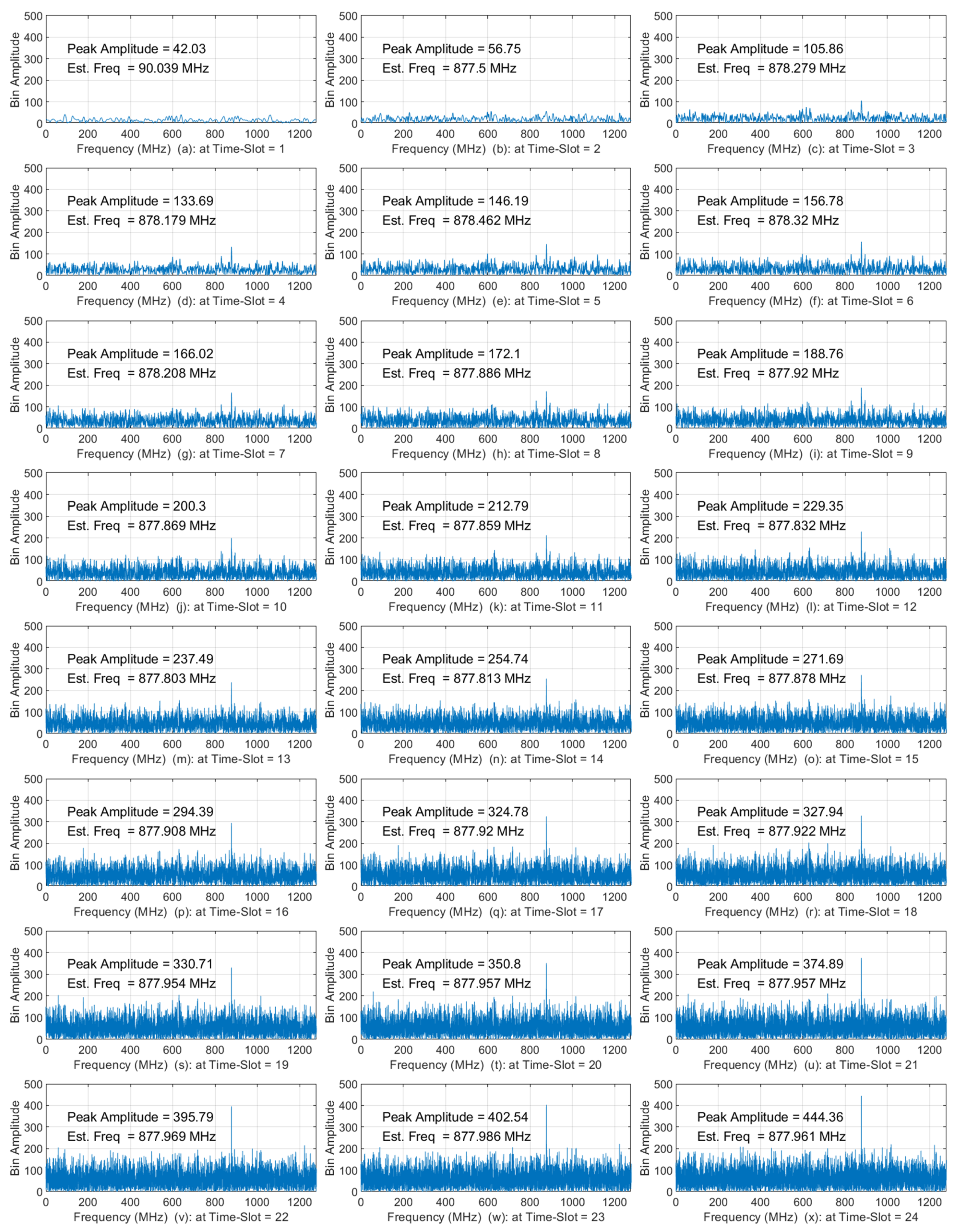
4.1. Examples to Demostrate the Comcept of AIRS
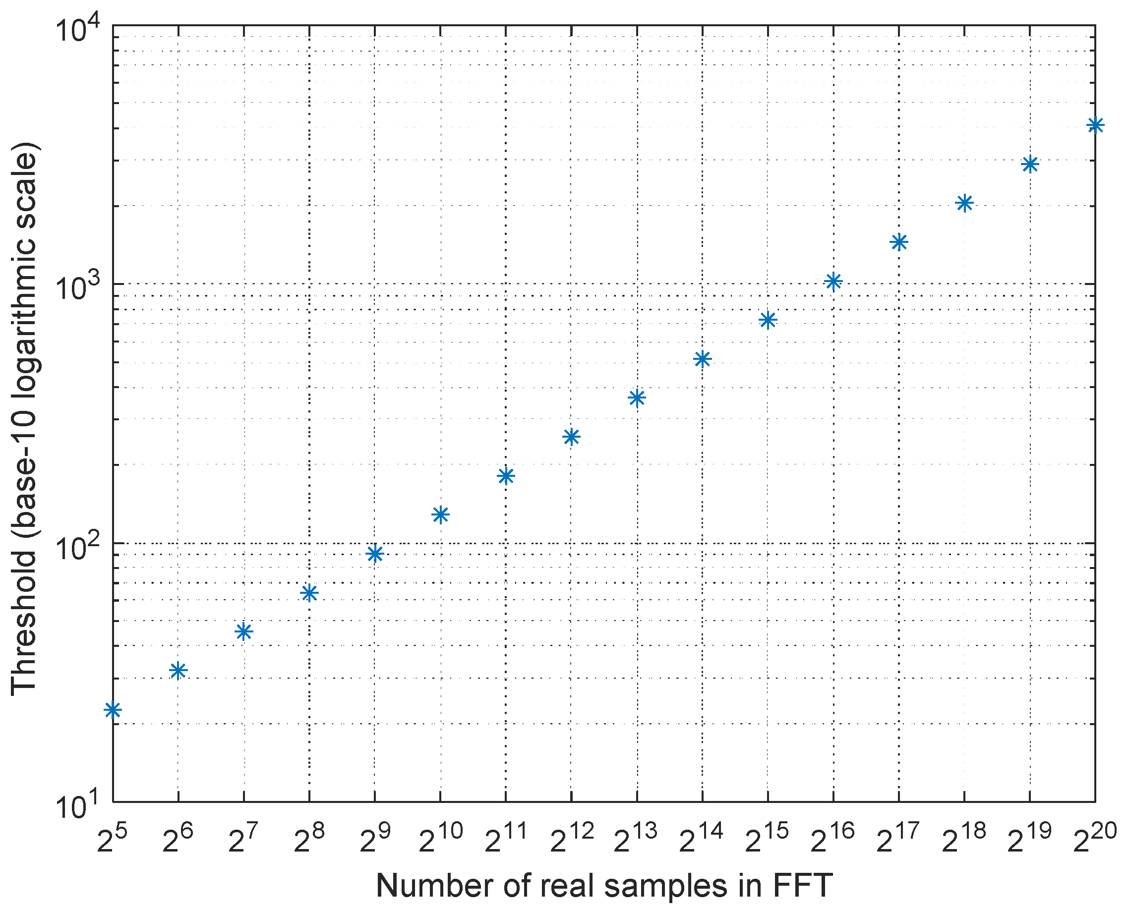
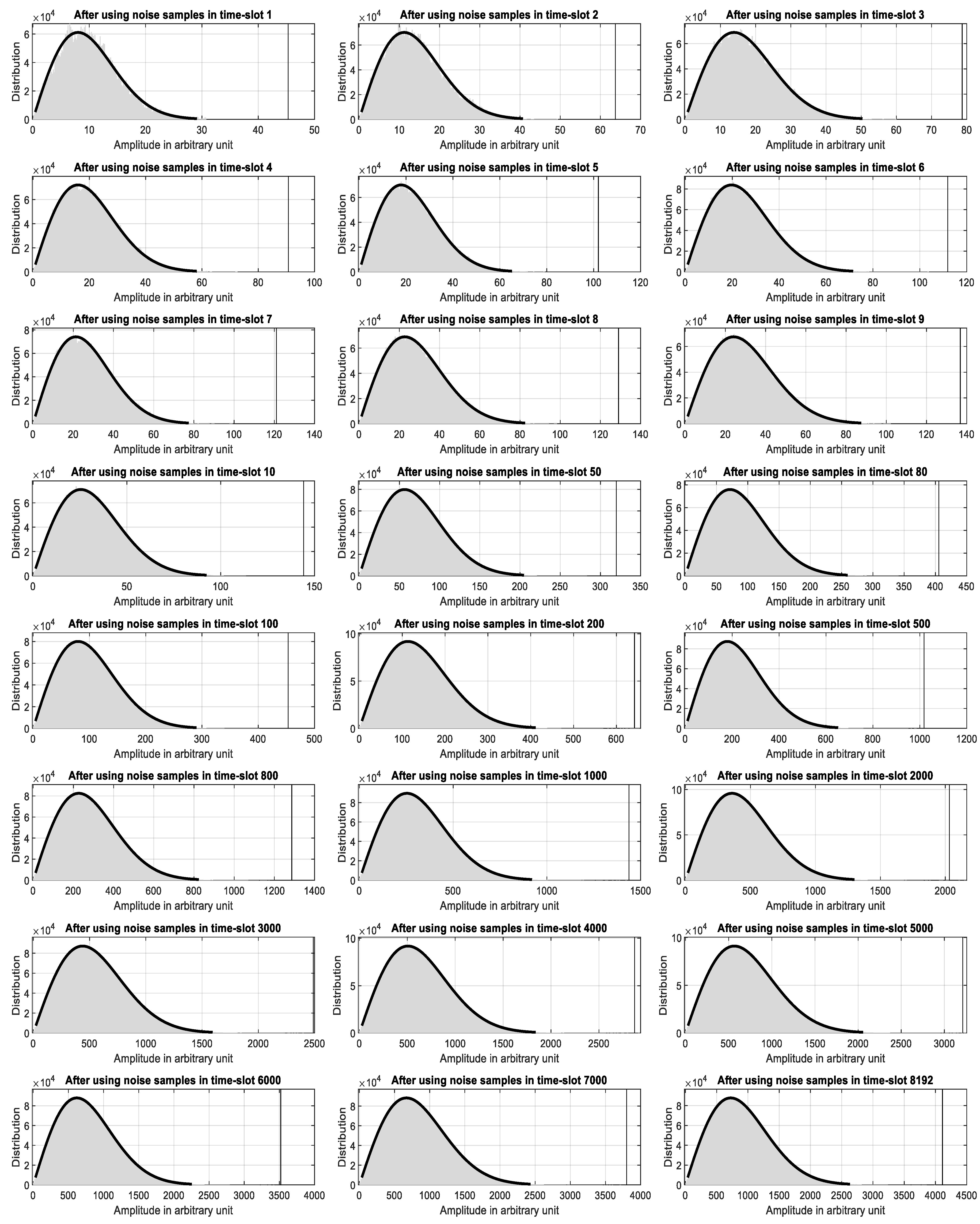
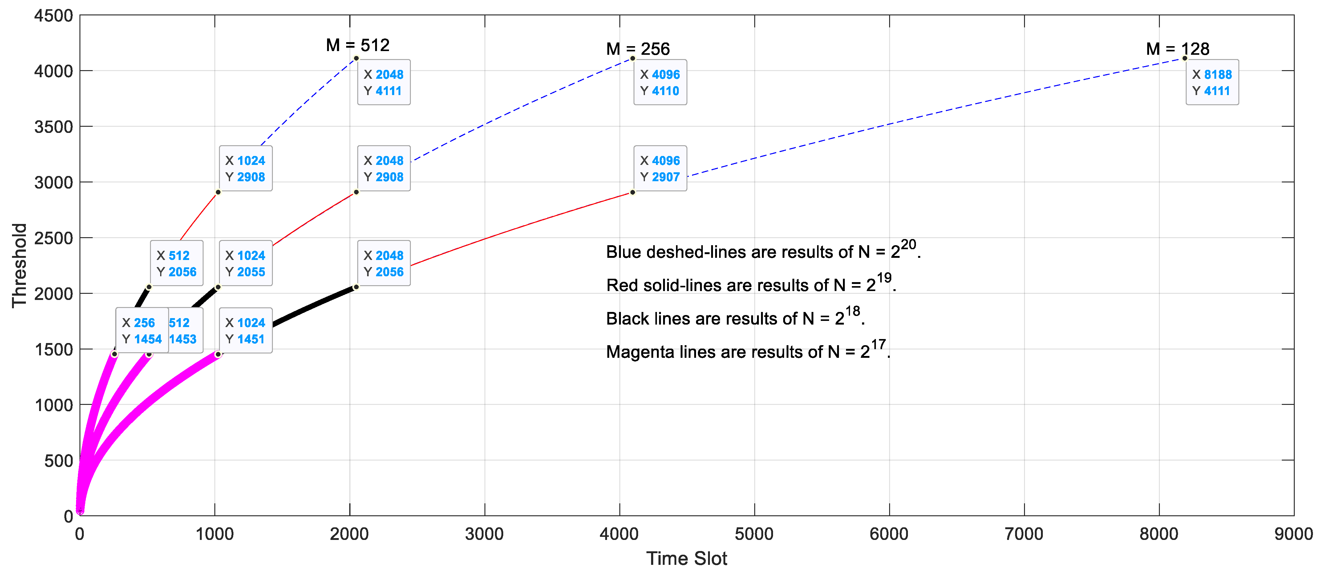
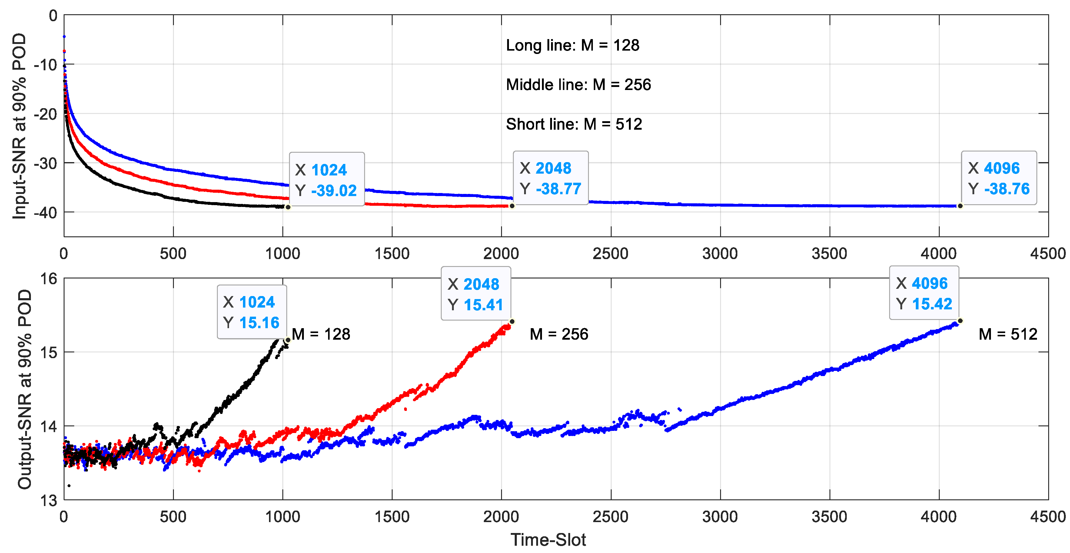
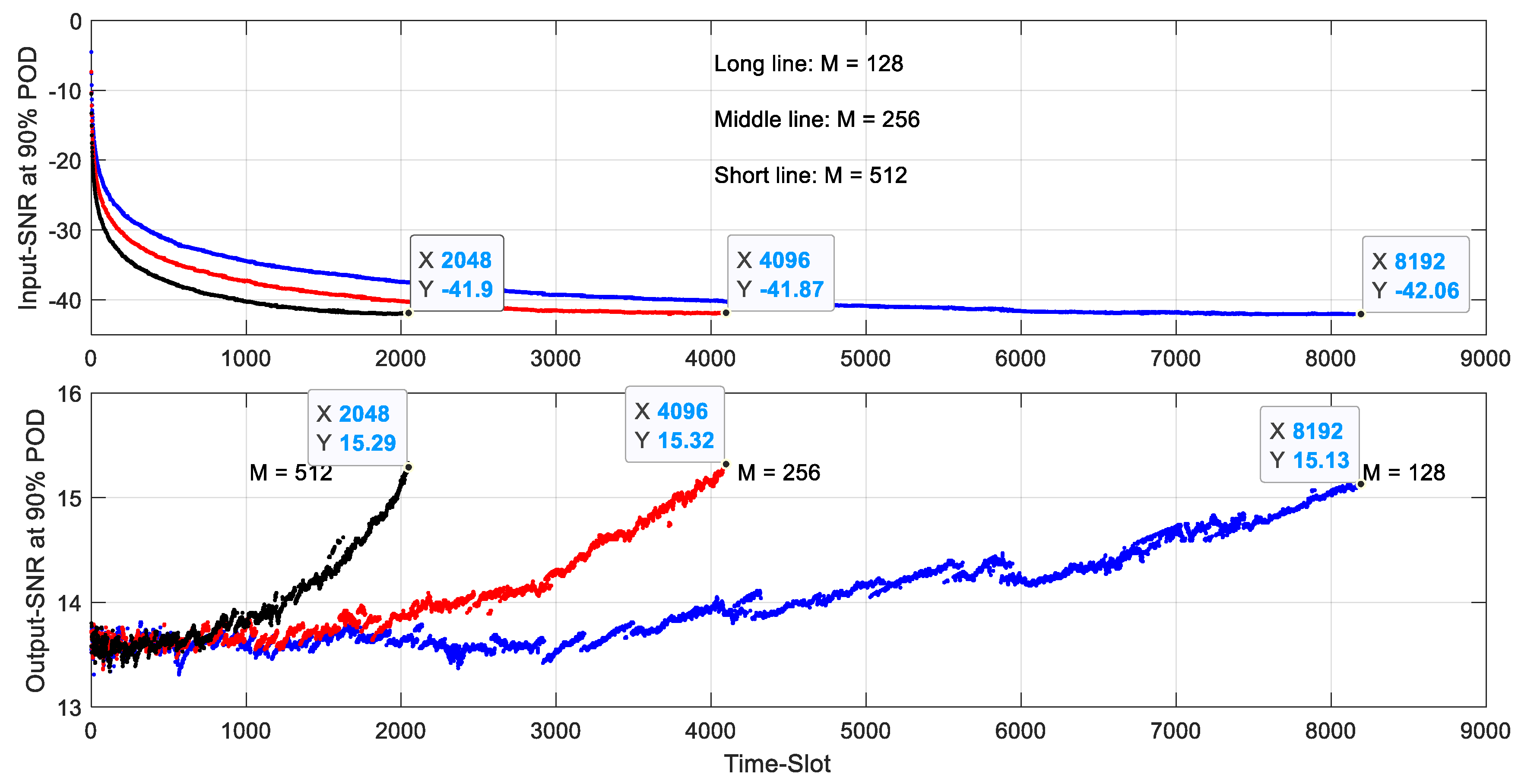
4.2. Thresholds of 90% POD with of 10−7 in AIRS Using Different Number of Time-Slot Data
- The number of frequency-bins equals to and ;
- In each case, the number of real noise samples in a time-slot equals 128, 256 and 512, respectively.
- 1.
- For a predefined number of frequency-bins in TTFT, to obtain the same threshold level, the total number of noise samples used in the calculations should be the same, even though the samples of time-slots can be different. For example, when the number of frequency-bins is , in order to reach the same threshold 4111, number of samples are needed irrespective of how the partition of the real noise samples is done in a time-slot. This result can help us to determine how to partition the samples in time-slots based on
- The required TMR, and/or
- The available hardware resources in the embedded system.
- 2.
- The threshold versus time-slot is independent to the predefined number of bins in TTFT, and only depends on how to partition samples in a time-slot. This is because when calculating the threshold in a given time-slot, the Gaussian-distributed noise samples make the contribution to all bins after being multiplied by the phase rotation factors and -point FFTs. Although for different the phase rotation factors are different, these factors do not introduce any new noise. So, when is fixed, for the same time-slot the threshold should be the same regardless of how many predefined frequency-bins in the TTFT. This result allows us to keep just one set of threshold tables in AIRS for a given , when the method is implemented in an embedded system. For example, we just use the dashed-line results in Figure 6 in following simulations.
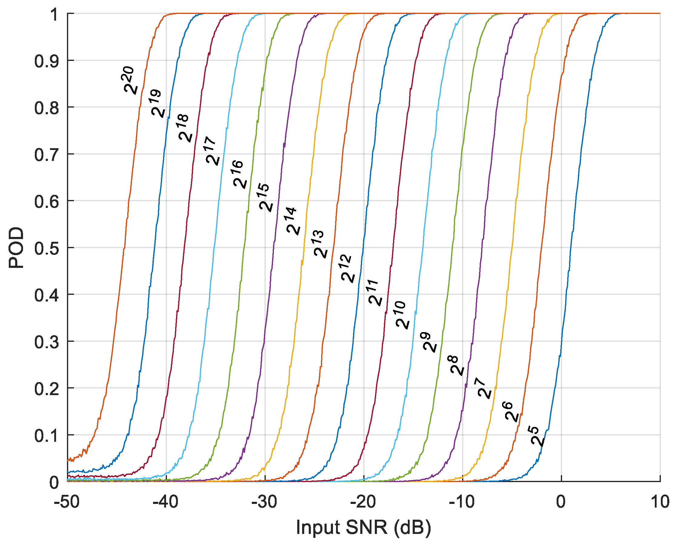
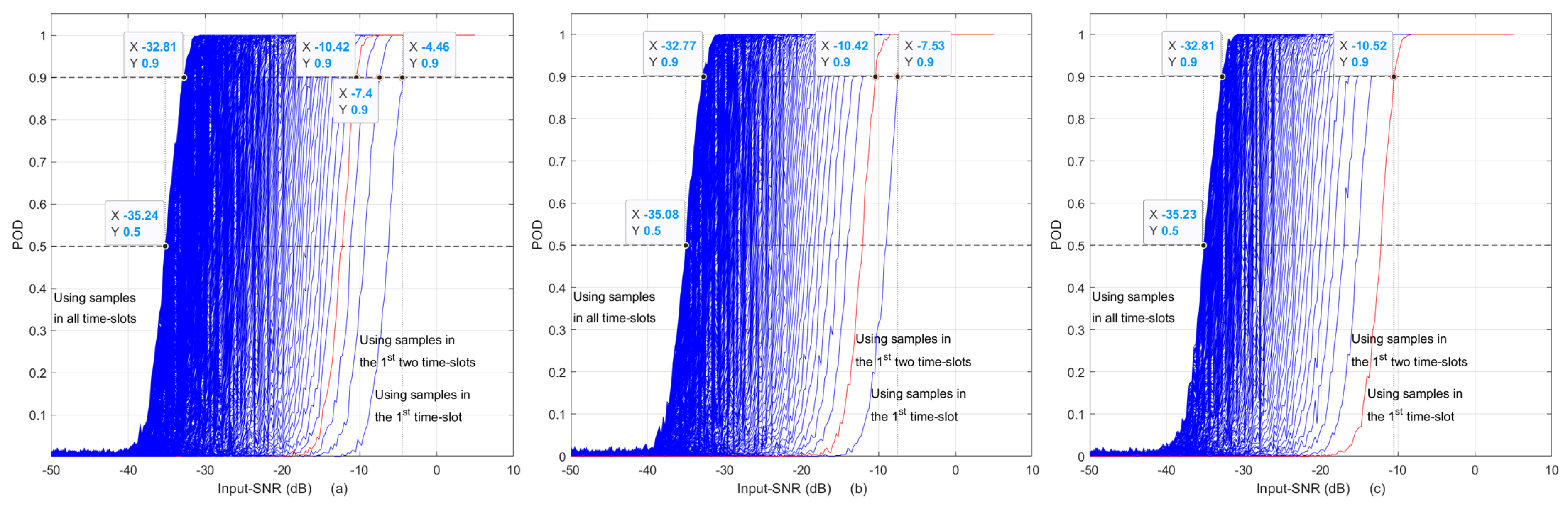
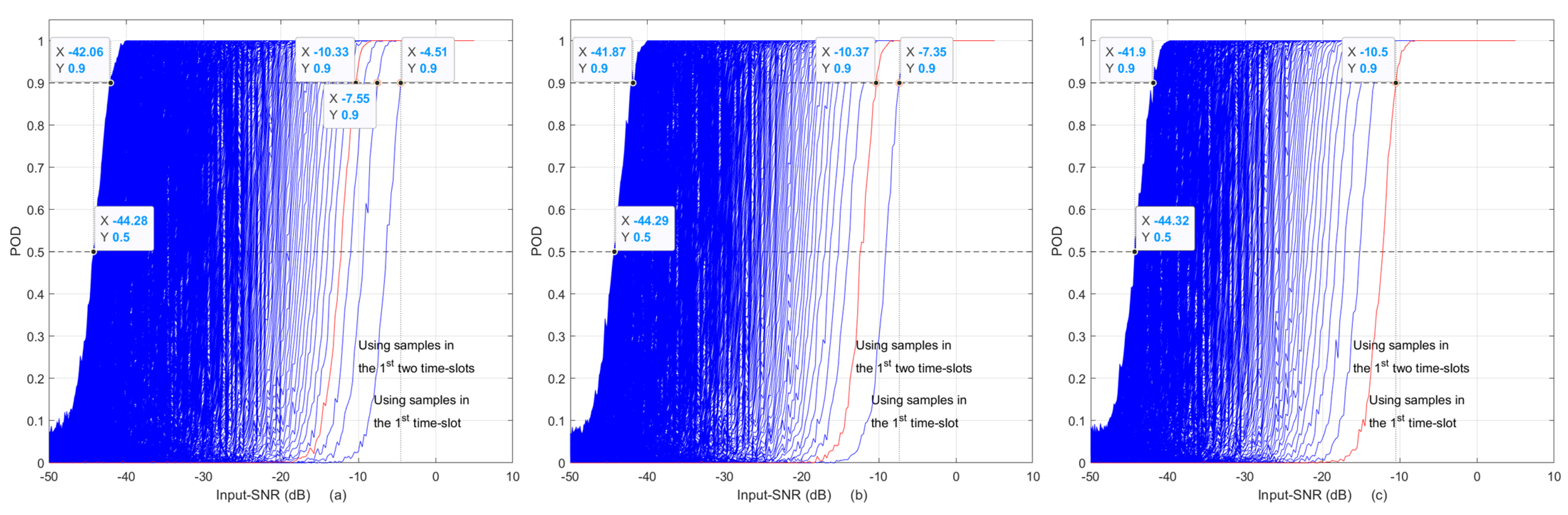
5. The POD with of 10−7 versus Input-SNR in AIRS for CW Signal Detection
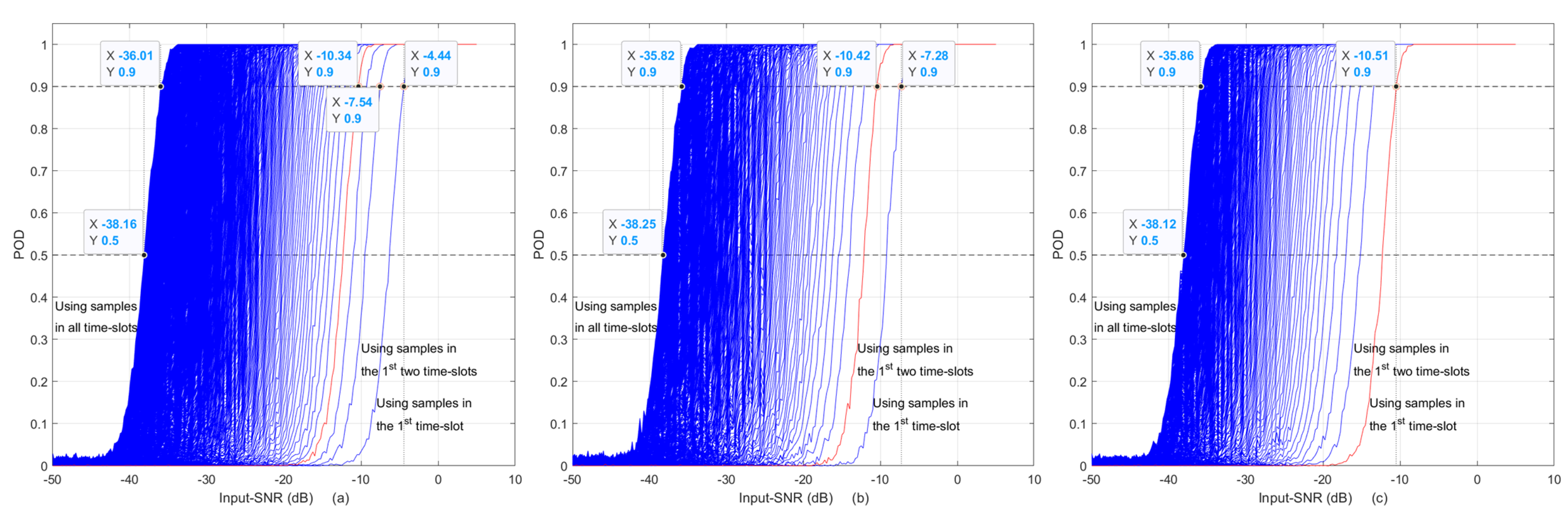
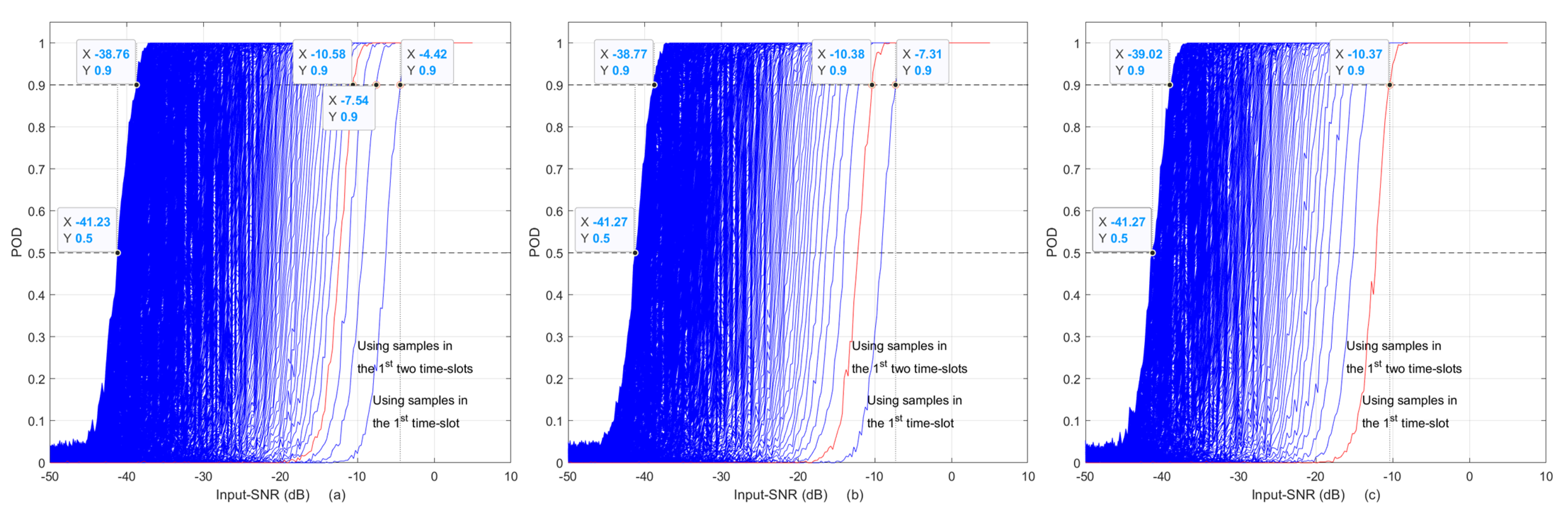
- As more time-slot samples are used, the required Input-SNR is reduced for a given POD. However, the rate of reduction decreases, as shown in Figure 7. Curves get more crowded as Input-SNR decreases.
- When samples in all the time-slots are used, the left-end curves of the three subplots in Figure 7 are all the same as the -POD curve shown in Figure 2, and the required Input-SNR for 90% POD is about −32.8 dB as given in the Table 2. This is the expected result, since using all the time-slot data in AIRS is the same as using -point FFT.
- As long as the same amount of samples are used in AIRS, it produces the same POD curve. For example, the red curve of four time-slots with in Figure 7a is the same as the red curve of two time-slots with in (b) and also is the same as the red curve of the first time slot with in (c). The required Input-SNRs for 90% POD of these three curves are listed in the figure, which are −10.42, −10.42 and −10.52 dB, respectively.
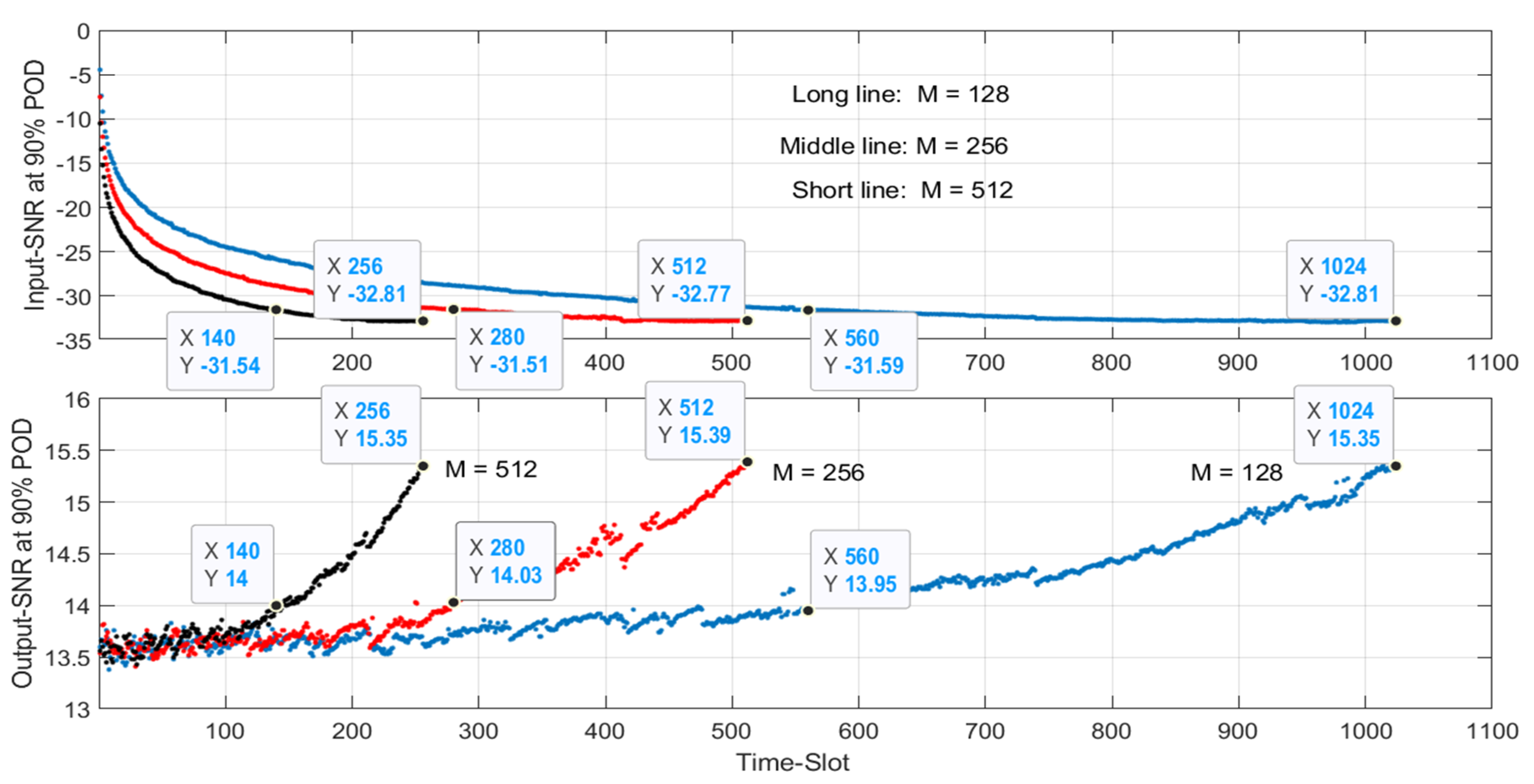
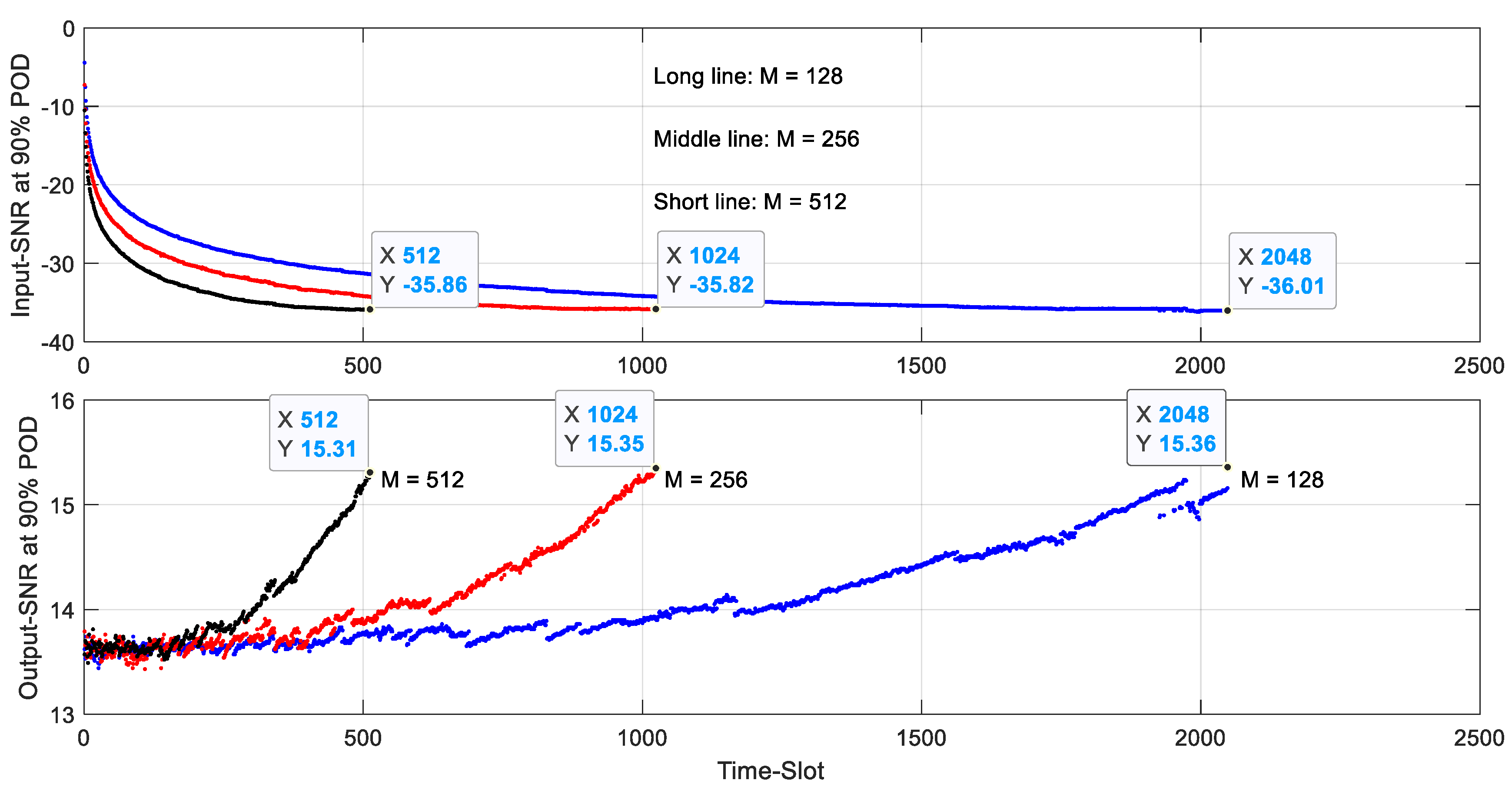
- The required minimum Output-SNRs are about the same, as long as the same number of samples is used in the AIRS, regardless of how the partition of the samples in a time-slot is done. For example, as shown in the bottom subplot of Figure 8, to detect signal at −31.5 dB Input-SNR with 90% POD, AIRS needs minimum of −14 dB Output-SNR, which needs samples from 560, 280 and 140 time-slots when and , respectively. Here the Output-SNR is defined as:where is the index of a time-slot, and can be viewed as AIRS-processing gain, which is equivalent to the FFT progressing gain discussed in Section 2.
- Figure 8 also shows that for AIRS, the minimum required Output-SNR is about 15.4 dB for 90% POD with of when all samples are used regardless of how the samples are partitioned in a time-slot. This is similar to the results given in Table 2. However, the AIRS can be more flexible to detect a signal using much less time-samples and maintain good TMR and FMR. Table 8 shows the TMR and FMR with different and combinations used in this study.
- All the above observations can also be found in
6. Narrow and Wideband Signal Detections Using AIRS
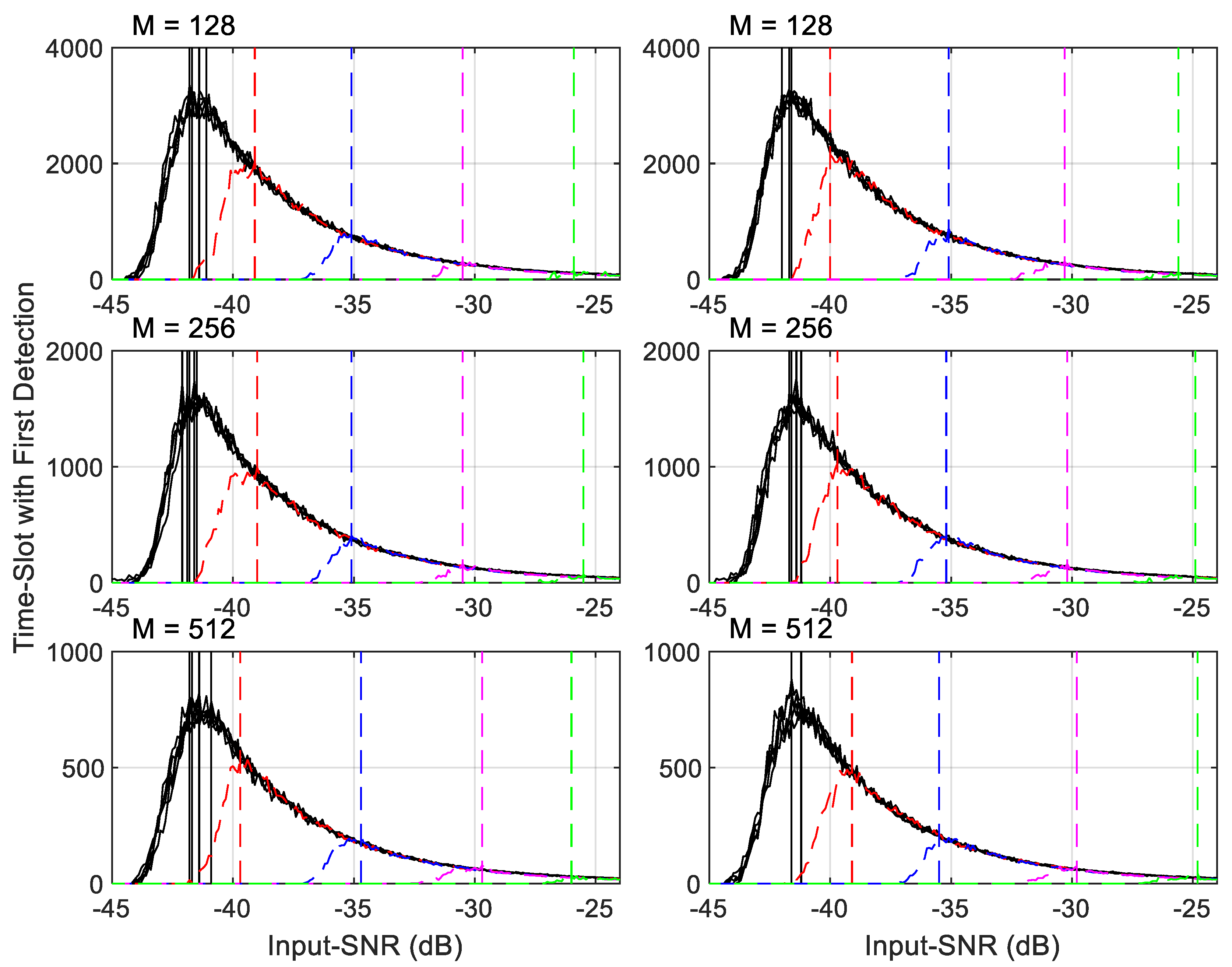
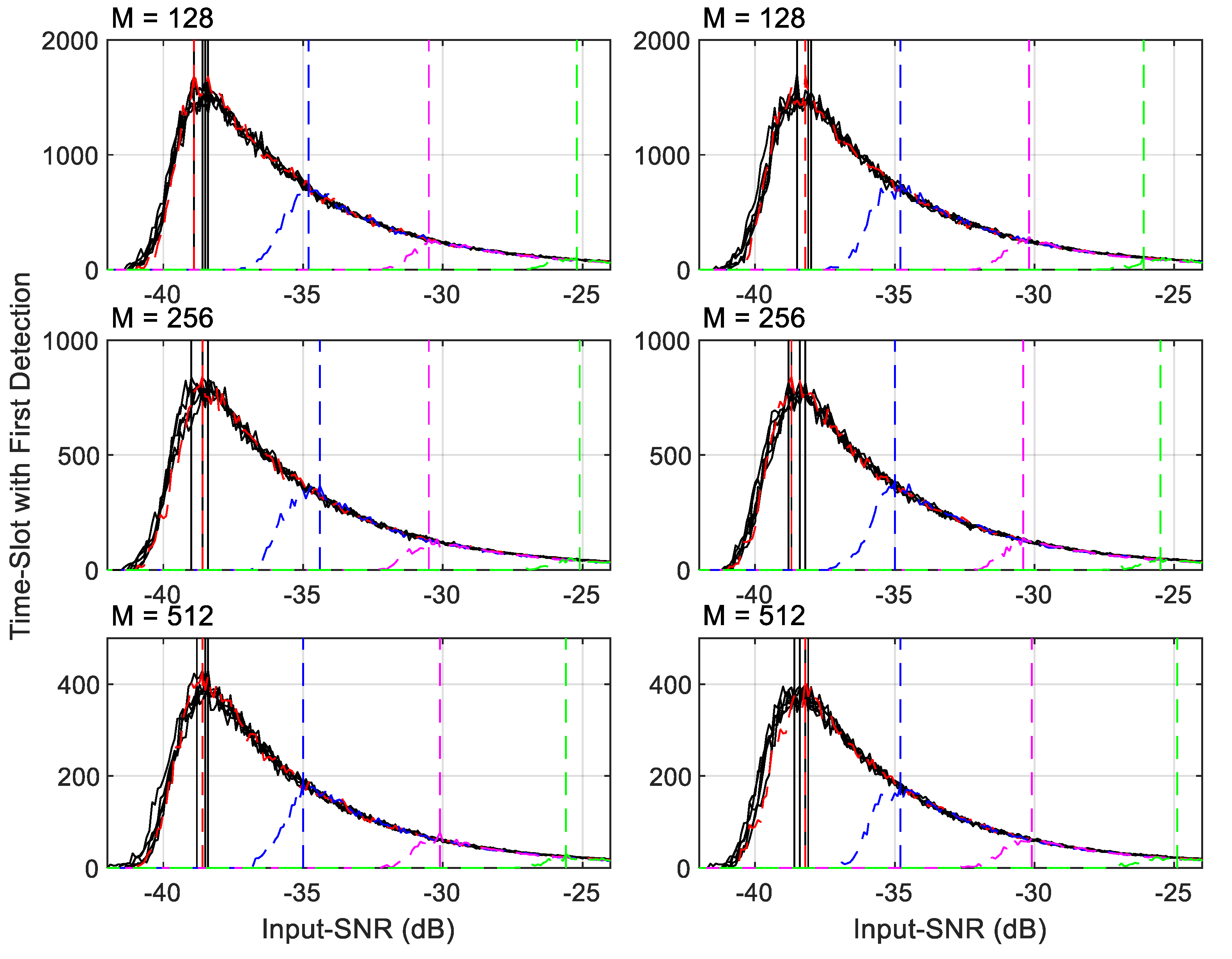
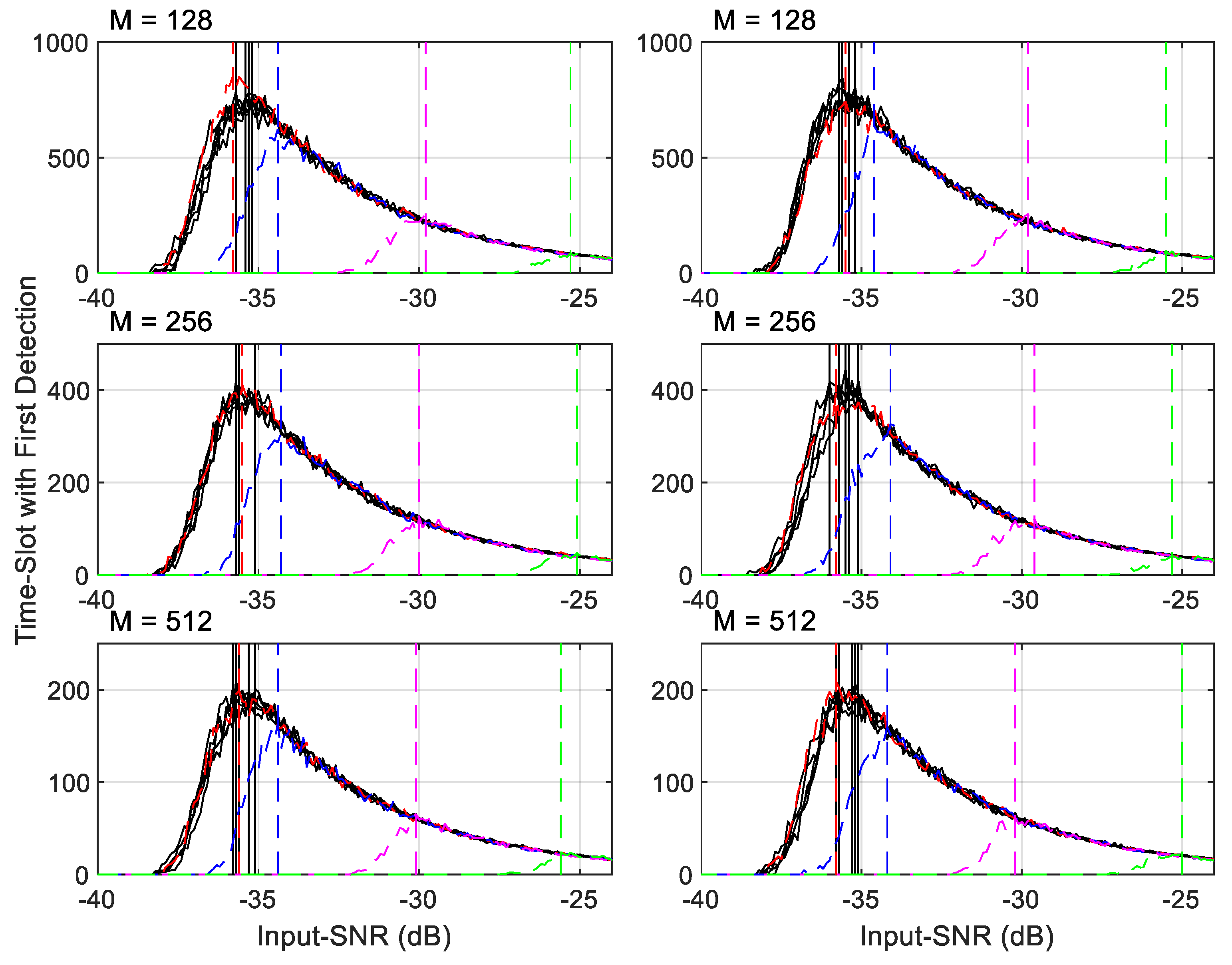
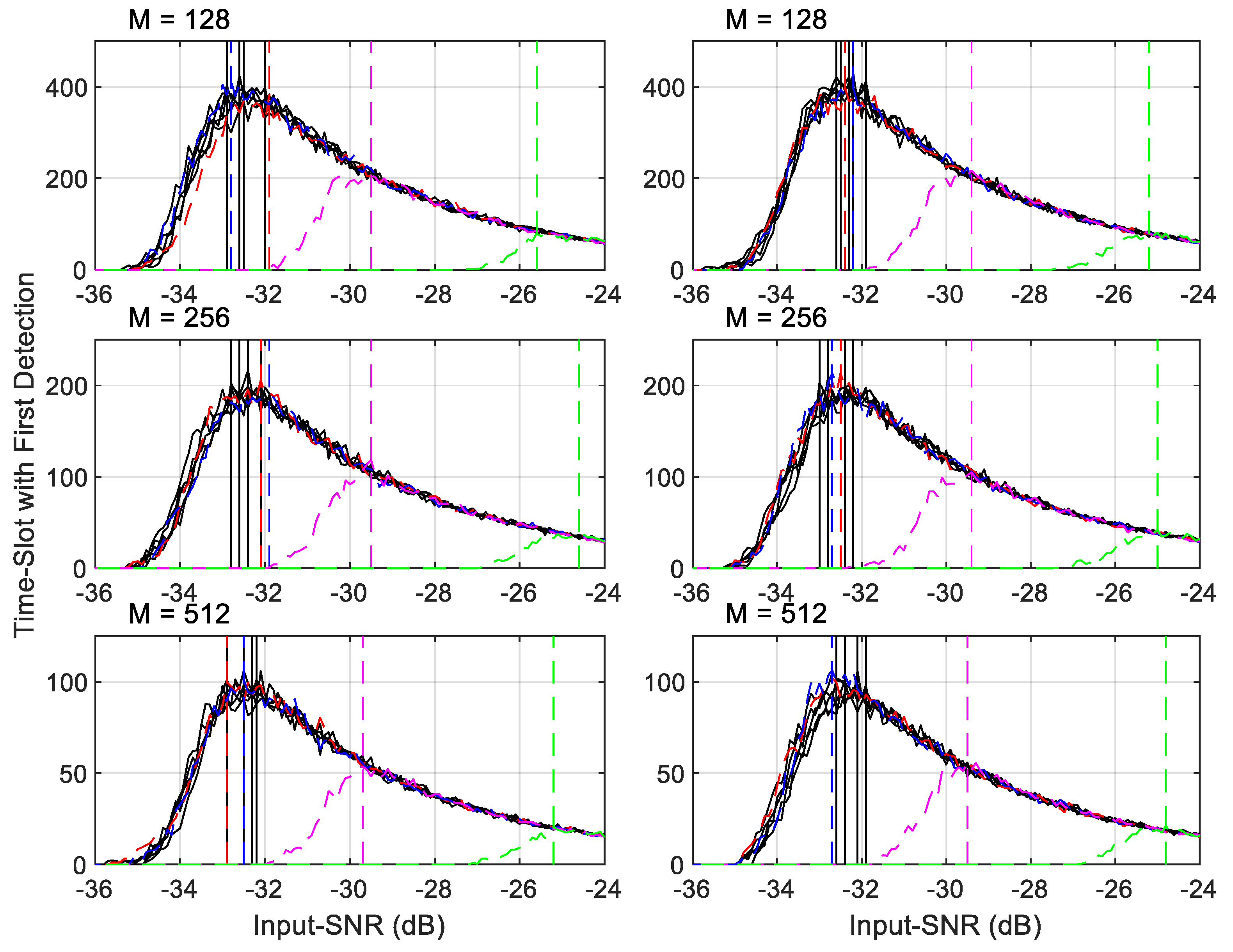
6.1. Input-SNR against Time-Slot That Has the First Detection
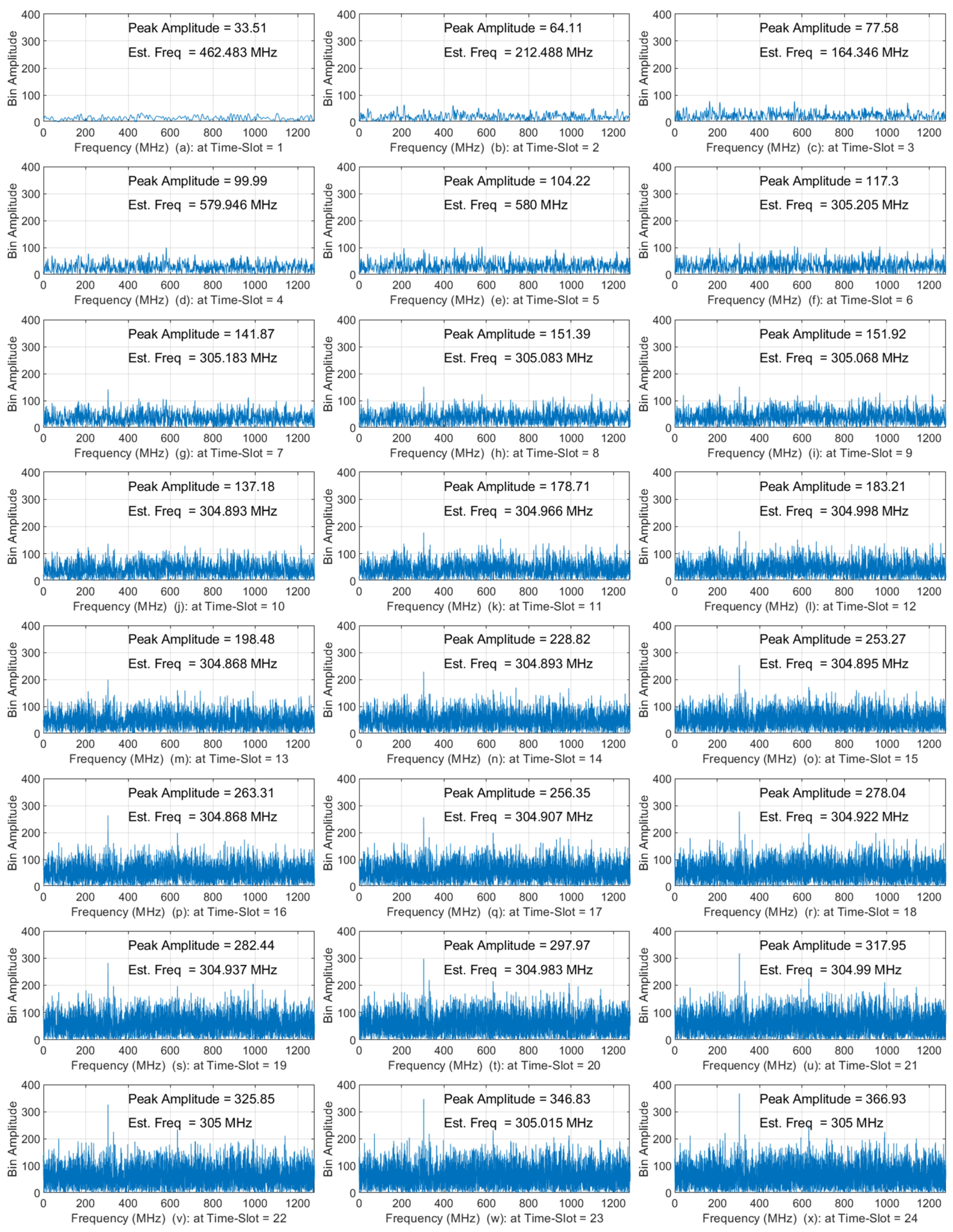
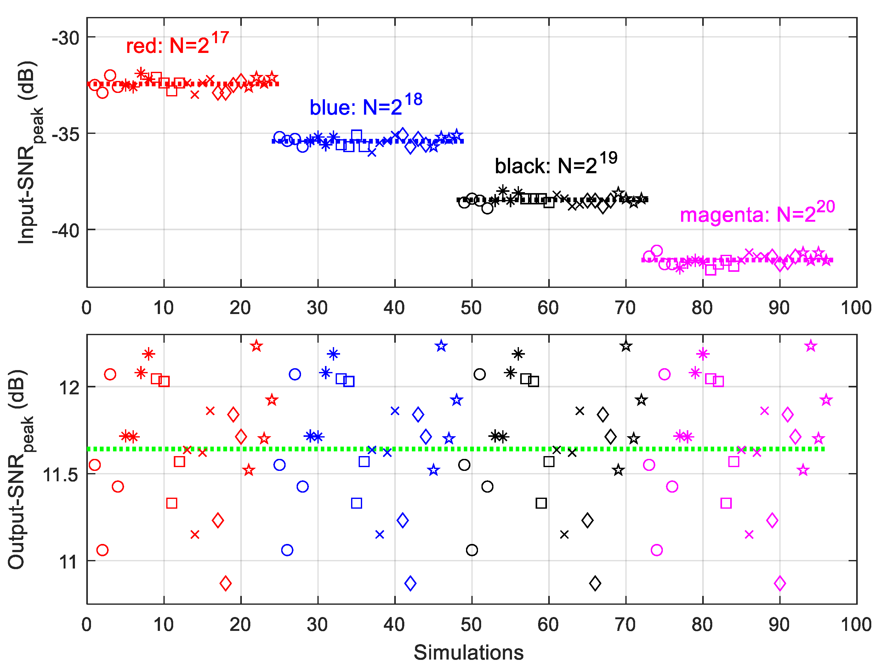
- For a given signal in Table 9, an Input-SNR vs. the time-slot having the first detection curve can be divided into two sections by the value, called Input-SNRpeak, on the curve, which is indicated by a solid or dashed vertical line. (More on Input-SNRpeak will be discussed later.)
- ○
- Before the Input-SNRpeak, the required time-slot numbers are increased as the Input-SNR decreases. In this range, the signal-power accumulation is faster than that of the noise. However, we can see that more time-slots are needed to detect lower Input-SNR signals, as the curves are in a concave shape.
- ○
- After the Input-SNRpeak, the required time-slot numbers are quickly reduced. The reason for this is faster accumulation of noise than the signal, and the detections happen only occasionally.
- ○
- When the Input-SNR is less than about −45 dB, there is no detection.
- For the first 5 narrow band signals in Table 9, shown in black-lines in the figure,
- AIRS can detect them at about −42 dB of Input-SNR level. This is the same results given in Table 2 that the minimum required Input-SNR for is −41.9 dB for 90% POD with of .
- The required time-slot numbers at Input-SNRpeak are less than for a given . This shows that the AIRS can start detecting narrow band signal using less than half of the real-samples that -point FFT needs.
- It is obvious that AIRS is much more efficient than -point FFT to detect signals when Input-SNR is higher than Input-SNRpeak. AIRS requires much less real-samples compared to the total bin size and it gives very good TMR (see Table 8) that the traditional FFT with large-bin numbers cannot achieve.
- For last 4 signals in Table 9, when the FMBW increases the AIRS is less capable of detecting them compared to detecting the narrow band signals. The reason for this will be discussed later. However, AIRS still can quickly detect them at lower than −25 dB Input-SNR with samples from a very small number of time-slots.
- Comparing the three subplots in Figure 15, the required time-domain samples are about the same at a given Input-SNR. It does not depend on the method of partitioning the samples in a time-slot. This is an anticipated result as the threshold in each time-slot depends only on the total noise samples used in the calculation.
6.2. Explanation of Wideband Signal Detection in AIRS
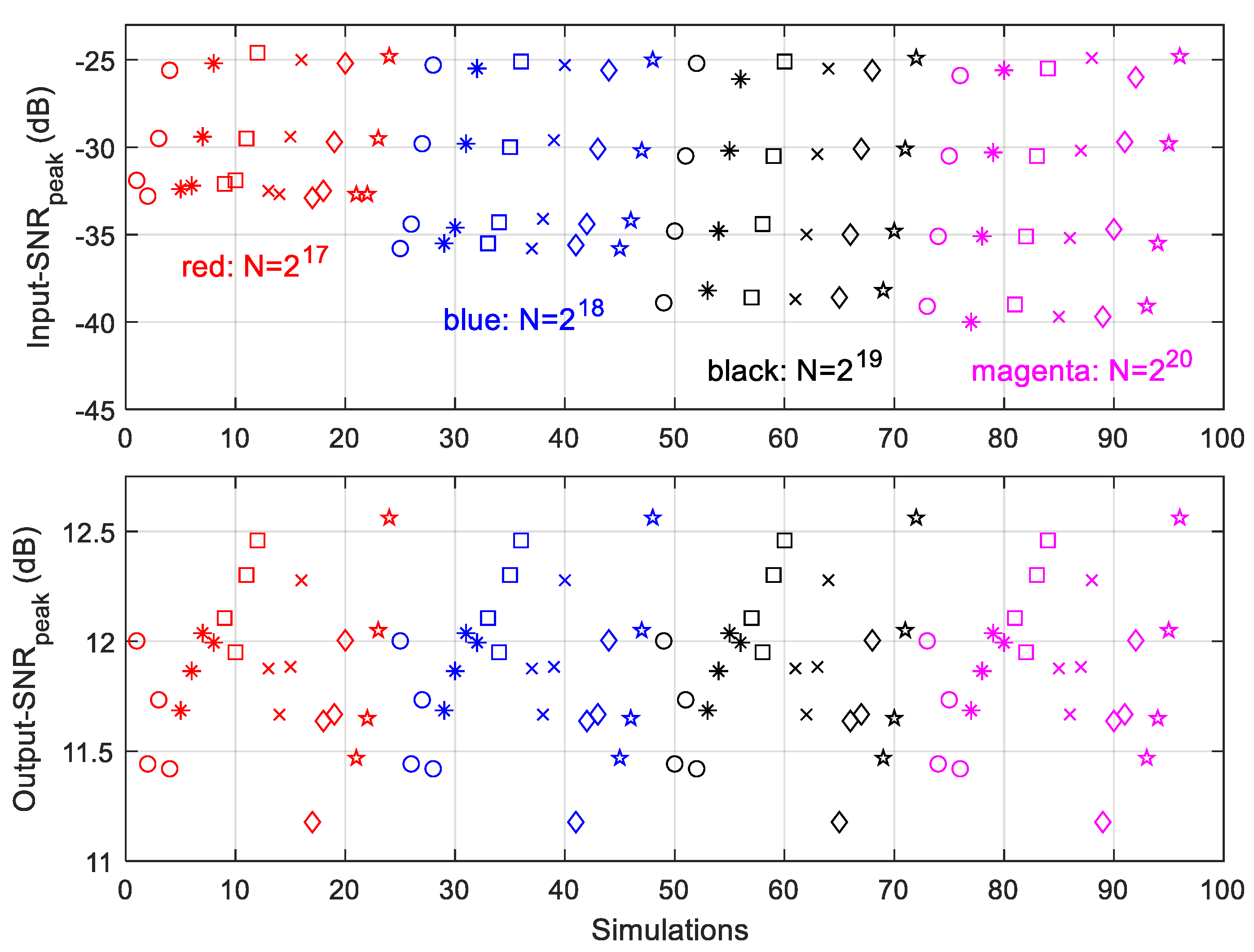
6.3. The Input-SNRpeak and Output-SNRpeak for Narrow-Band Signals
- When is doubled the Input-SNRpeak reduces 3 dB.
- The Output-SNRpeak values are in between 10.75 to 12.3 dB, and the averaged Output-SNRpeak is about 11.64 dB.
- The Output-SNRpeak discussed here is related to the time-slot that has the first detection of narrow-band signals with Input-SNRpeak, when of is considered. The Output-SNR discussed in Section 5 was to consider 90% POD for CW signal. However, what is important to note is that at the Input-SNRpeak levels given in Table 11, which are about the same levels of Input-SNR in Table 2, AIRS only needs less than real-samples to detect these signals, while FFT needs all the real-samples. The reason is that AIRS uses the time-slot-based thresholds, which only invokes the noise up to that specific time-slot.
- We also want to emphasize that the advantage of the AIRS processing is that it can detect signals using the currently available samples for the frequency-bins without waiting for the availability of all the samples. This offers a feasible way of hardware implementation when a large number of samples are available from a high-speed ADC.
7. Conclusions
Author Contributions
Funding
Institutional Review Board Statement
Informed Consent Statement
Data Availability Statement
Acknowledgments
Conflicts of Interest
Appendix A. The Comparison between Results Obtained by the MATLAB FFT Function and the BFFT Code

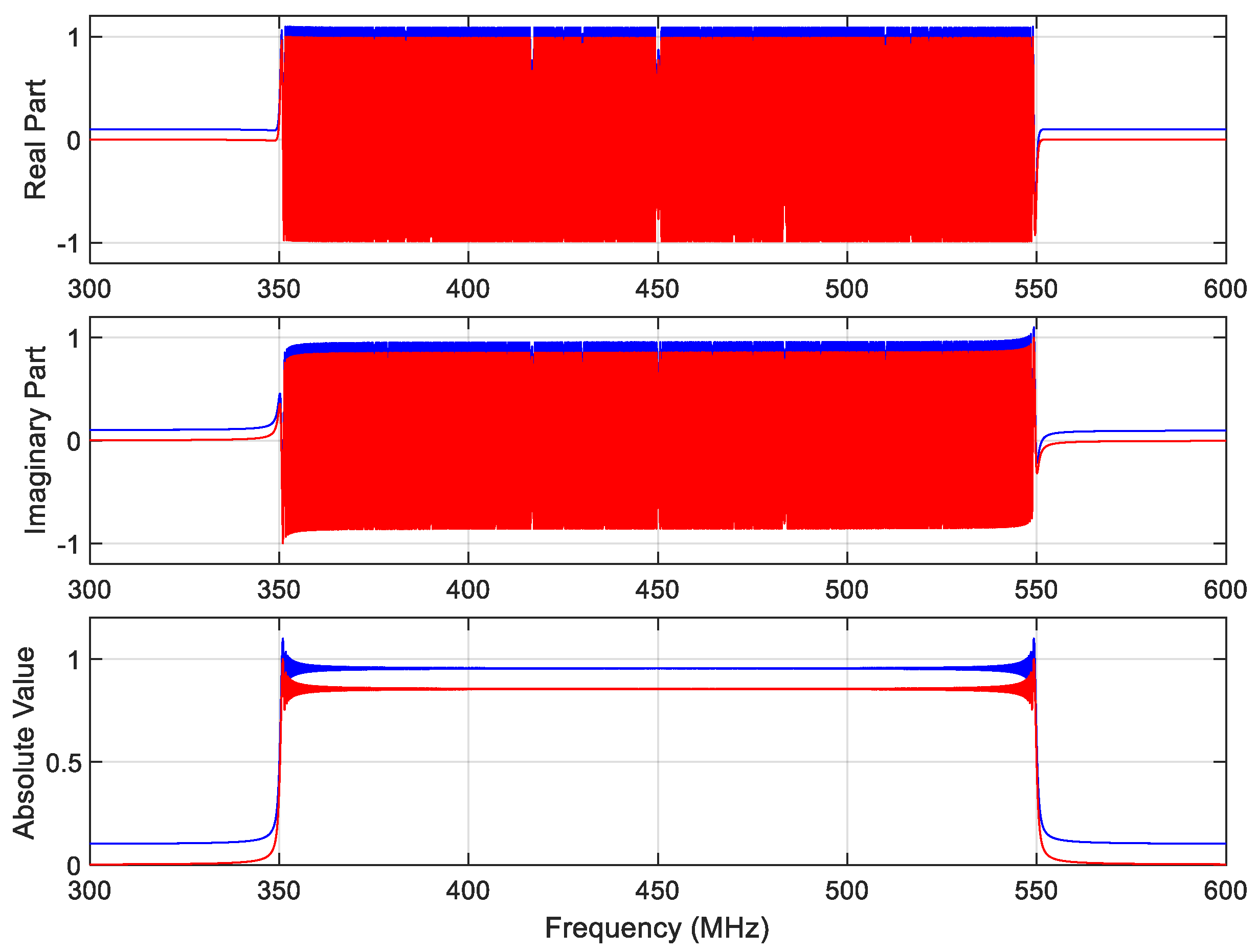
| Figure | Number of Samples | Signal | Duration (mSec) | Chirp Start (MHz) | Carrier End (MHz) | ADC (GHz) | Input-SNR (dB) | BFFT | |
|---|---|---|---|---|---|---|---|---|---|
| A1 | Chirp | 0.4096 | 350.1 | 550.1 | 2.56 | 100 | 4096 | 256 | |
| A2 | Chirp | 0.2048 | 650.1 | 860.1 | 2.56 | 0 | 4096 | 128 | |

Appendix B. Acronym List
| ADC | Analog-to-Digital Converter |
| AIRS | Accumulatively Increasing Receiver Sensitivity |
| BFFT | Blocking FFT |
| BW | Bandwidth |
| CW | Continuous Wave |
| DFT | Discrete Fourier Transform |
| DRX | Digital Receiver |
| FFT | Fast Fourier Transform |
| FMBW | Frequency Modulation Bandwidths |
| FMCW | Frequency Modulated Continuous Wave |
| FPGA | Field Programmable Gate A19rray |
| FMR | Frequency Measurement Resolution |
| IBW | Instantaneous Bandwidth |
| Input-SNR | Input Signal-to-Noise Ratio |
| LIP | Low Probability Intercept |
| Output-SNR | Output Signal-to-Noise Ratio |
| POD | Probability of Detection |
| PW | Pulse Width |
| TMR | Time-of-arrival Measurement Resolution |
| TTFT | Time-to-Frequency Transform |
References
- Pace, P.E. Detecting and Classifying Low Probability of Intercept Radar, 2nd ed.; Artech House: Norwood, MA, USA, 2009. [Google Scholar]
- Boashash, B. Time-Frequency Signal Analysis and Processing, 2nd ed.; Academic Press: Oxford, UK, 2016. [Google Scholar]
- Haneche, H. Compressed Sensing in Mobile Systems, Networking and Internet Architecture [cs.NI]. Ph.D. Thesis, University of Science and Technology Houari Boumediene, Bab Ezzouar, Algeria, 2020. [Google Scholar]
- Haneche, H.; Boudraa, B.; Ouahabi, A. A new way to enhance speech signal based on compressed sensing. Measurement 2020, 151, 107117. [Google Scholar] [CrossRef]
- Wu, C.; Rajan, S. Fast Fourier sampling for ultra-wide band digital receiver applications. In Proceedings Volume 8753, Wireless Sensing, Localization, and Processing VIII; International Society for Optics and Photonics: Bellingham, WA, USA, 2013; Volume 8753. [Google Scholar] [CrossRef]
- Layne, D. Receiver Sensitivity and Equivalent Noise Bandwidth, High Frequency Electronics, J2014. Available online: https://www.highfrequencyelectronics.com/index.php?option=com_content&view=article&id=553:receiver-sensitivity-and-equivalent-noise-bandwidth&catid=94&Itemid=189 (accessed on 23 October 2021).
- Green, H.E. A theoretical examination of tangential signal to noise ratio. IEEE Trans. Microw. Theory Tech. 1991, 39, 566–567. [Google Scholar] [CrossRef]
- Packard, H. The Criterion for the Tangential Sensitivity Measurement, Application Note 956-1. 1990. Available online: http://www.hp.woodshot.com/hprfhelp/4_downld/lit/diodelit/an956-1.pdf (accessed on 25 September 2021).
- Tsui, J.B.Y. Special Design Topics in Digital Wideband Receivers; Artech House: Norwood, MA, USA, 2010. [Google Scholar]
- Neri, F. Introduction to Electronic Defence Systems, 3rd ed.; Artech House: Norwood, MA, USA, 2018. [Google Scholar]
- Hedge, J.; Tsui, J.B.Y.; Sharpin, D. Sensitivity of digital electronic warfare receivers. IEEE Conf. Aerosp. Electron. 1990, 3, 981–984. [Google Scholar] [CrossRef]
- Xilinx, Zynq UltraScale+ RFSoc, ZCU208 Evaluation Board User Guide. Available online: https://www.xilinx.com/content/dam/xilinx/support/documentation/boards_and_kits/zcu208/ug1410-zcu208-eval-bd.pdf (accessed on 6 September 2021).
- Annino, B. SFDR Considerations in Multi-Octave Wideband Digital Receivers, Analog Dialogue, Volume 55, No. 1, January 2021. Available online: https://www.analog.com/media/en/analog-dialogue/volume-55/number-1/sfdr-considerations-in-multi-octave-wideband-digital-receivers.pdf (accessed on 6 September 2021).
- Cheng, C.; Lin, D.M.; Liou, L.L.; Tsui, J.B. Electronic Warfare Receiver with Multiple FFT Frame Sizes. IEEE Trans. Aerosp. Electron. Syst. 2012, 48, 3318–3330. [Google Scholar] [CrossRef]
- Kanders, H.; Mellqvist, T. One Million-Point FFT. Master’s Thesis, Electrical Engineering Department of Electrical Engineering, Linköping University, Linköping, Sweden, 2018. [Google Scholar]
- Li, Y.; Chen, H.; Xie, Y. An FPGA-based four-channel 128k-point FFT processor suitable for space-borne SAR. Electronics 2021, 10, 816. [Google Scholar] [CrossRef]
- Agarwal, A.; Hassanieh, H.; Abari, O.; Hamed, E.; Katabi, D.; Arvind. High-throughput implementation of a million-point sparse Fourier Transform. In Proceedings of the 2014 24th International Conference on Field Programmable Logic and Applications (FPL), Munich, Germany, 2–4 September 2014; pp. 1–6. [Google Scholar] [CrossRef]
- Xu, P.K.; Xu, F.Y. A real-time spectral analysis method and its FPGA implementation for long-sequence signals. Meas. Sci. Technol. 2020, 31, 035006. [Google Scholar] [CrossRef]
- Naval Air Warfare Center Weapon Division. Electronic Warfare and Radar Systems Engineering Handbook, NAWCWD TP 8347, 4th ed.; Naval Air Warfare Center Weapon Division: Point Mugu, CA, USA, 2013. [Google Scholar]
- Wu, C.; Krishnasamy, D.; Elangage, J. Hardware Implementation and RF High-Fidelity Modeling and Simulation of Compressive Sensing Based 2D Angle-of-Arrival Measurement System for 2–18 GHz Radar Electronic Support Measures. Sensors 2021, 21, 6823. [Google Scholar] [CrossRef] [PubMed]
- Richardson, L. The Sliding Window Discrete Fourier Transform. Ph.D. Thesis, Carnegie Mellon University, Pittsburgh, PA, USA, 2019. [Google Scholar] [CrossRef]
- Viswanathan, M. Chi Square Distribution–Demystified, GaussianWaves: Signal Processing for Communication Systems, 11 September 2022. Available online: https://www.gaussianwaves.com/2012/09/chi-squared-distribution (accessed on 16 January 2022).
| FFT Length | 32 | 64 | 128 | 256 | 512 | 1024 |
| Threshold | 22.67 | 32.16 | 45.52 | 64.21 | 90.90 | 128.42 |
| Threshold from [9] | 22.92 | 32.07 | 45.26 | 64.24 | 90.66 | 128.33 |
| FFT Length | 32 | 64 | 128 | 256 | 512 | 1024 | 216 | 217 | 218 | 219 | 220 |
| Min. Input-SNR (dB) | 3.3 | 0.4 | −2.7 | −5.7 | −8.7 | −11.7 | −29.8 | −32.8 | −35.9 | −38.9 | −41.9 |
| Min. Output-SNR (dB) | 15.3 | 15.6 | 15.4 | 15.4 | 15.4 | 15.4 | 15.4 | 15.4 | 15.3 | 15.3 | 15.3 |
| Time-Slot | 0 | 1 | ⋯ | k | ⋯ | K − 1 |
|---|---|---|---|---|---|---|
| u | 0, 1, 2, 3, …… M − 1 | |||||
| 0, 1,… M − 1 | ||||||
| M | After -independent -point FFTs, the first set of frequency-domain data that will be added to frequency-bins. | |
| 0 | ||
| 1 | ||
| 2 | ||
| M | frequency-bins. | |
| 0 | ||
| 1 | ||
| 2 | ||
| M | The set of frequency-domain data that will be added to frequency-bins. | |
| 0 | ||
| 1 | ||
| 2 | ||
| m | The last set of frequency-domain data that will be added to frequency-bins. | |
| 0 | ||
| 1 | ||
| 2 | ||
| 128 | 256 | 512 | |
| 50 (nSec) 19,531 (Hz) | 100 (nSec) 19,531 (Hz) | 200 (nSec) 19,531 (Hz) | |
| 50 (nSec) 9765.6 (Hz) | 100 (nSec) 9765.6 (Hz) | 200 (nSec) 9765.6 (Hz) | |
| 50 (nSec) 4882.8 (Hz) | 100 (nSec) 4882.8 (Hz) | 200 (nSec) 4882.8 (Hz) | |
| 50 (nSec) 2441.4 (Hz) | 100 (nSec) 2441.4 (Hz) | 200 (nSec) 2441.4 (Hz) | |
| FMBW (Hz) | 1 | 100 | 1000 | 10 K | 100 K | 1 M | 10 M | 100 M | |
|---|---|---|---|---|---|---|---|---|---|
| Colors and line styles in Figure 15 and Figure 16 | Black solid | Black solid | Black solid | Black solid | Black solid | Red dashed | Blue dashed | Magenta dashed | Green dashed |
| Linear FMCW FMBW (Hz) | 1 | 100 | 1000 | 10 K | 100 K | 1 M | 10 M | 100 M | |
|---|---|---|---|---|---|---|---|---|---|
| Frequency BW/sample (Hz) | 1.95 × 10⁻⁷ | 1.95 × 10⁻⁵ | 1.95 × 10⁻⁴ | 4.77 × 10⁻⁴ | 1.95 × 10⁻³ | 1.95 × 10⁻² | 0.195 | 1.95 | 19.5 |
| Samples having frequency BW equals to bin width | 1.25 × 10+10 ≫N | 1.25 × 10+8 ≫N | 1.25 × 10+7 ≫N | 5.12 × 10+2 >N | 1.25 × 10+6 ≈N | 1.25 × 10+5 <N | 1.25 × 10+3 ≪N | 1250 ≪N | 125 ≪N |
| Convert 3rd row data into time-slots | 97,656,250 ≫K | 976,563 ≫K | 97,656 ≫K | 40,000 >K | 9766 ≈K | 977 <K | 98 ≪K | 9.77 ≪K | 0.98 ≪K |
| Averaged Input-SNRpeak (dB) | −32.44 | −35.42 | −38.67 | −41.58 |
| Averaged Output-SNRpeak (dB) | 11.64 | |||
Publisher’s Note: MDPI stays neutral with regard to jurisdictional claims in published maps and institutional affiliations. |
© 2022 by the authors. Licensee MDPI, Basel, Switzerland. This article is an open access article distributed under the terms and conditions of the Creative Commons Attribution (CC BY) license (https://creativecommons.org/licenses/by/4.0/).
Share and Cite
Wu, C.; Tang, T.; Elangage, J.; Krishnasamy, D. Accumulatively Increasing Sensitivity of Ultrawide Instantaneous Bandwidth Digital Receiver with Fine Time and Frequency Resolution for Weak Signal Detection. Electronics 2022, 11, 1018. https://doi.org/10.3390/electronics11071018
Wu C, Tang T, Elangage J, Krishnasamy D. Accumulatively Increasing Sensitivity of Ultrawide Instantaneous Bandwidth Digital Receiver with Fine Time and Frequency Resolution for Weak Signal Detection. Electronics. 2022; 11(7):1018. https://doi.org/10.3390/electronics11071018
Chicago/Turabian StyleWu, Chen, Taiwen Tang, Janaka Elangage, and Denesh Krishnasamy. 2022. "Accumulatively Increasing Sensitivity of Ultrawide Instantaneous Bandwidth Digital Receiver with Fine Time and Frequency Resolution for Weak Signal Detection" Electronics 11, no. 7: 1018. https://doi.org/10.3390/electronics11071018
APA StyleWu, C., Tang, T., Elangage, J., & Krishnasamy, D. (2022). Accumulatively Increasing Sensitivity of Ultrawide Instantaneous Bandwidth Digital Receiver with Fine Time and Frequency Resolution for Weak Signal Detection. Electronics, 11(7), 1018. https://doi.org/10.3390/electronics11071018