Article

An Efficient Recursive Multibeam Pattern Subtraction (MPS) Beamformer for Planar Antenna Arrays Optimization

Department of Computer Engineering, College of Computers and Information Technology, Taif University, P.O. Box 11099, Taif 21944, Saudi Arabia
*
Author to whom correspondence should be addressed.
Electronics 2022, 11(7), 1015; https://doi.org/10.3390/electronics11071015
Submission received: 1 March 2022 / Revised: 19 March 2022 / Accepted: 23 March 2022 / Published: 24 March 2022
(This article belongs to the Section Networks)

Abstract

:
In this paper, a new beamforming technique for planar two-dimensional arrays is proposed for optimizing the sidelobe levels (SLLs) by using recursive multibeam pattern subtraction (MPS) technique. The proposed MPS beamformer is demonstrated and its convergence to lower SLL values is investigated and controlled. The performance analysis has shown that the proposed MPS beamformer can effectively reduce the SLL down to less than −50 dB relative to the mainlobe level utilizing the major sidelobes information in the radiation pattern. In addition, the proposed MPS beamformer can be applied to any planar array geometry such as rounded corners rectangular arrays provided that the original array pattern contains sidelobe peaks. The comparison with recent related techniques has shown that the proposed beamformer provides faster convergence time. On the other hand, the proposed technique provides lower sidelobe levels which cannot be achieved by efficient tapering windows for planar two-dimensional arrays. Finally, the scanning performance of the proposed MPS beamformer is demonstrated and the simulation results show solid and consistent SLL levels over the whole angular range from the broadside to endfire directions of the array.

1. Introduction

1.1. Background and Motivation

Antenna arrays have an important role in the current and future revolution in wireless communications systems and applications including mobile radio communications, satellite communications, wireless networks, Internet of things (IoT), radar, sonar, and many others [1,2,3,4,5,6,7,8,9]. For example, the efficient delivery and reception of signals in the current fifth generation (5G) mobile communication networks depend on multi-input multi-output (MIMO) techniques based on antenna arrays and beamforming to achieve very high capacity and data rates in the range of few giga bits per second [2,3]. The higher data rate and capacity are also necessary for IoT networks where huge number of sensors require to communicate efficiently with reduced interference levels through onboard antenna arrays. In addition, sonar and radar systems are basically based on narrow beams originated from antenna arrays with very low sidelobe levels (SLLs) of −50 dB or less to scan the intended angular spaces efficiently without interception by unwanted clutter [8]. Therefore, any improvement in the antenna array performance is necessary for most applications and SLL reduction is one of the most important performance improvements in antenna array systems. There are several techniques that can be applied to reduce the unwanted sidelobe radiation ranging from simple tapered beamforming windows [10,11,12,13] up to advanced evolutionary optimization techniques [14,15,16,17,18,19,20,21,22,23,24,25,26,27]. Tapered windows were naturally designed for linear arrays and provide straightforward solution for SLL reduction with limited capabilities while arrays with small or limited sizes can be optimized by using evolutionary optimization techniques based on heuristic or population methods [14], or nature-based techniques such as ant colony [15], firefly optimization [16], and particle swarm optimization [17,18]. In addition, there are many other optimization techniques including flower pollination [19], grey wolf optimization [20], weed colonization [21], and cuckoo search algorithm [22] that were developed for optimizing the beam patterns of antenna arrays including beam synthesis and interference cancellation. However, there is a main limitation of the evolutionary optimization techniques where there are many input parameters that require selection and tuning especially for large array sizes making it difficult to guarantee the algorithm convergence [28]. Applications that require three-dimensional beamforming such as 5G wireless networks, satellite communications, radar and sonar systems utilize planar two-dimensional arrays which sometimes are massive, and it becomes very difficult to apply complex evolutionary optimization techniques in this case as the convergence is not guaranteed at reasonable processing time. On the other hand, simple tapered windows could be applied directly for planar two-dimensional arrays where the element feeding amplitudes are determined from deterministic equation, however the achieved SLL is also limited and could not be improved due to these fixed window functions. In addition, efficient controlled tapers such as Dolph-Chebyshev and Kaiser windows are naturally designed for linear arrays and were extrapolated and applied to planar concentric circular arrays as in [12,13], however, the achieved SLL is not deep enough as required in some applications such as radar scanning systems to avoid unwanted clutter [29,30]. Other optimization techniques such as in [31] includes the interelement spacing as a parameter to effectively reduce the SLL, however, the array design once completed cannot be reconfigured and thus lacks flexibility or adaptation for the varying environments. On the other hand, arrays of massive antenna elements such as large planar arrays require fast and responsive beamforming techniques especially in nonstationary communication environments. Recently, the idea of sidelobes self-refining in the uniform antenna arrays by beamspace processing has achieved deep SLL for linear one-dimensional arrays as in [32,33,34] where single or multiple secondary mainlobes are formed and their patterns are weighted and subtracted from the original pattern to suppress the intended sidelobes. The sequential sidelobe damping (SSD) algorithm in [32] has optimized linear arrays using single beam subtraction which is sequentially repeated to damp or suppress the remaining sidelobes in the radiation pattern, so after several iteration cycles, the SLL could be effectively reduced. The SSD algorithm, although have stable convergence profiles and faster convergence time compared with evolutionary optimization techniques, suffers from slower convergence where more than 1000 iteration cycles are required to achieve deep SLL of −50 dB or less for planar arrays. The SSD algorithm has been improved by simultaneous sidelobe reduction (SSR) algorithm in [33] and adaptive SSR in [34] for massive linear arrays. The convergence speed in these two algorithms has been improved and could find the optimum weights five times faster than the SSD algorithm where the optimization of massive linear arrays formed by several hundreds of antenna elements could be achieved in few iterations as in the adaptive SSR algorithm. However, these three algorithms were proposed to mainly optimize linear arrays which can be extended or modified to work with planar arrays efficiently after investigation and controlling its performance. Therefore, in this paper, an optimization technique for planar arrays beamforming and SLL reduction is proposed and analyzed using multibeam pattern subtraction (MPS). The proposed beamforming technique is extensively investigated to achieve complete algorithm convergence over wide range of planar array sizes and angular scanning range.

1.2. Paper Contribution

As the three-dimensional (3D) beamforming is necessary for many applications which utilizes planar arrays, therefore in this paper, an efficient beamforming technique is proposed to generate beam patterns with controlled SLL values. The proposed technique utilizes the unique patterns of sidelobes in the uniform feeding case to generate secondary mainlobes with the same levels of the sidelobes which are then weighted properly and subtracted from the original pattern and the process can be repeated to achieve the required SLL. The proposed MPS beamformer analyzes the sidelobes in each reduction cycle to find the proper corresponding weights to achieve the convergence. The algorithm is extensively investigated where its performance is analyzed at different array sizes and configurations, number of sidelobes adopted in the reduction process, convergence controlling and limitations, and scanning of the mainlobe and its effect on the SLL variation. The simulation results show that the proposed MPS beamformer can achieve deep SLL near −65 dB or less according to the number of number of iterations and can be applied to any planar array structure with different dimensions including rounded corners rectangular arrays. In addition, the proposed MPS beamformer has convergence speed that is more than five times compared with that of the SSD algorithm which is essential for real time beamforming using massive planar arrays. In addition, the array optimization can be achieved only one time to find the required weights at the broadside direction of the array, then can be rephased to generate scanning beams of the same SLL without re-optimization. This important feature greatly reduces the processing time until different SLL values are required.

1.3. Paper Organization

Section 2 demonstrates and models the proposed MPS beamforming technique for planar two-dimensional arrays while its performance is investigated in detail with several parameters in Section 3. In Section 4, the MPS beamformer is compared with efficient tapered windows and finally, Section 5 concludes the paper.

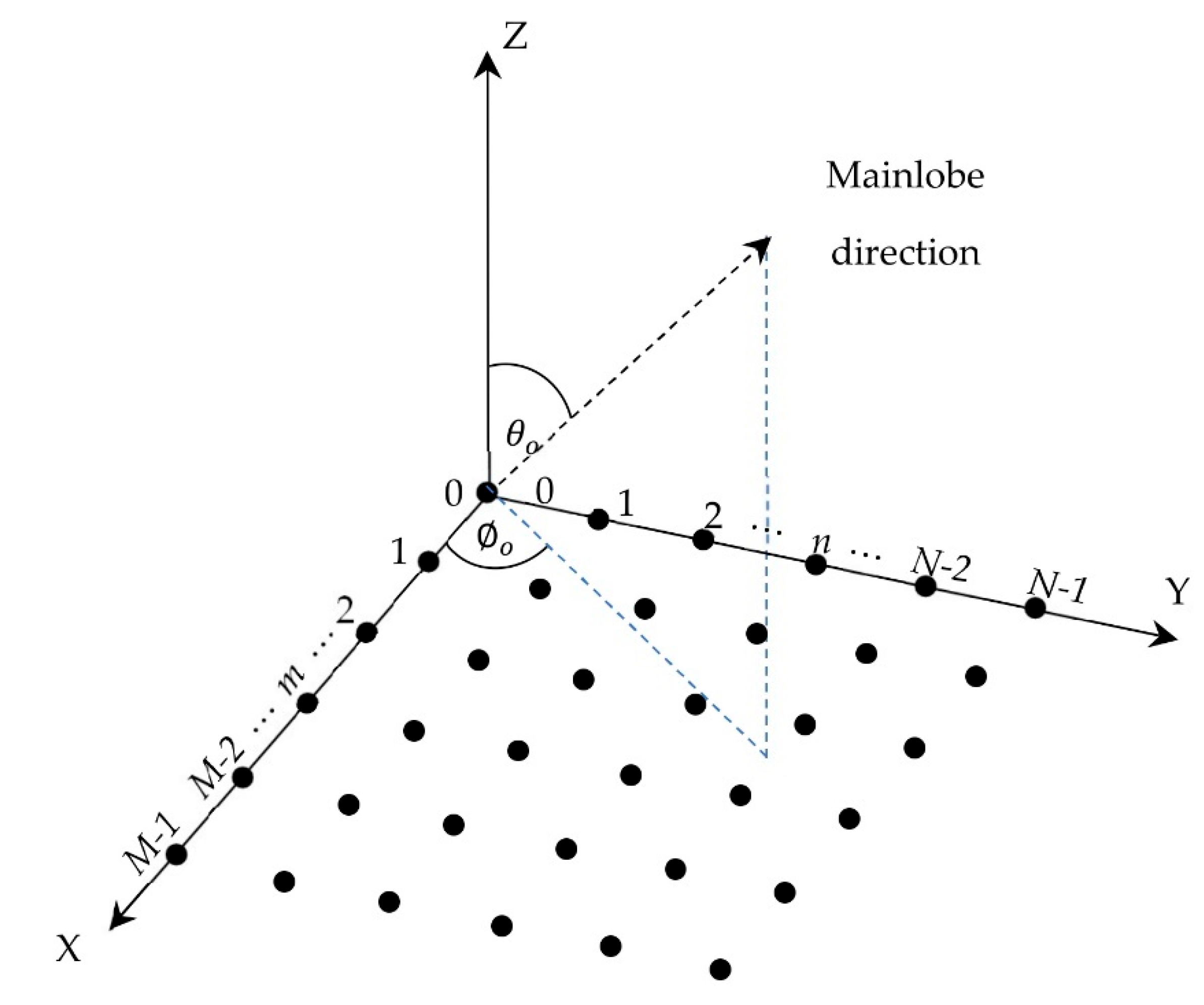
2. Multibeam Pattern Subtraction (MPS) Beamformer Modelling

In this section, the MPS beamformer is modelled and investigated. Assuming a rectangular array formed by M × N elements in the XY-plane as shown in Figure 1 where the antenna elements are interseparated by a half-wavelength distance ( λ / 2 ) as in most array designs.
A popular planar array design has rounded corners which can be simply inserted in the array model by including an array masking matrix μ . This structure gains the benefits of low sidelobe levels as in the concentric circular arrays but with suitable element distribution for more easier feeding of the antenna elements. The array center is located by a distance δ m , n (normalized to λ / 2 ) from m,n-th element which can be written as:
δ m , n = ( m ( M 1 ) / 2 ) 2 + ( n ( N 1 ) / 2 ) 2
where m = 0, 1, 2, …, M − 1, n = 0, 1, 2, …, N − 1 are the element location indices on the array plane.
The maximum normalized distance from the array center is given by:
δ M A X = ( ( M 1 ) / 2 ) 2 + ( ( N 1 ) / 2 ) 2
The array center has been chosen as a reference point to form the rounded-corners array structure by using the array masking matrix, μ , whose elements are given by:
μ m , n = { 1 ,     δ m , n δ T     0 ,   o t h e r w i s e  
where δ T is a normalized threshold distance that defines the array corners trim profile where δ T < δ M A X for circularly trimmed corners and δ T = δ M A X for the full rectangular array structure (no trimmed elements at the four array corners).
The array steering matrix which defines the relative phase shifts between elements is defined as follows:
S ( θ , ϕ ) = μ A ( θ , ϕ )
where is the Hadamard product (element-wise product) and   A ( θ , ϕ ) is the rectangular array steering matrix whose m,n-th element is given by:
a m , n ( θ , ϕ ) = e j π m 2 + n 2 cos ( ϕ ϕ m , n ) sin ( θ )
where ϕ m , n = tan 1 ( n m ) .
The array factor can be written as:
A F ( θ , ϕ ) = S U M ( W H S ( θ , ϕ ) )
where S U M ( ) is an operator in MATLAB that finds the sum of all elements in a matrix, H is the Hermitian operator, and W is the array weighting matrix.
For uniform feeding case, W is given by:
  W = S ( θ o , ϕ o )
which results in a mainlobe directed towards ( θ o , ϕ o ) .
For full rectangular arrays (all elements in μ are equal to 1), the sidelobes have identified peaks and the two major sets of them are located on two perpendicular planes centered around the mainlobe as shown in Figure 2 for uniformly feeding of 16 × 16 antenna array. We consider only the front side array pattern which is in the range 90 ° θ 90 ° where one mainlobe is generated while the back image pattern is always attenuated or damped by the practical antenna structures.
The number of sidelobes in these two major sidelobe planes in this visible angular range is given by:
n M , N = M + N 4
These major sidelobes are lined in the two perpendicular planes at ϕ = 0 ° and ϕ = 90 ° with highest SLL of approximately −13.26 dB. On the other hand, there are also many minor sidelobes located between these two major planes with highest SLL of approximately −26.43 dB. Therefore, we assume that the significant set of sidelobes for multibeam subtraction are α times the number of major sidelobes in Equation (8) or:
P = α ( M + N 4 )
The resulted SLL of the uniform feeding case can be improved by using weighted multibeam pattern subtraction where multi-mainlobes are formed and weighted at the same directions of sidelobes and subtracted from the main pattern with proper amplitude weighting. The process can be repeated to achieve the required SLL if the convergence of the process is guaranteed.
If the number of multibeams used for SLL reduction is P, then the resulting array factor after SLL reduction iterations (i) can be written as:
A F i + 1 ( θ , ϕ ) = A F i ( θ , ϕ ) β p = 1 P S U M ( A F i H ( θ p , ϕ p ) | N S ( θ p , ϕ p ) S ( θ , ϕ ) )
where A F i + 1 ( θ , ϕ ) is the resulted array factor after SLL reduction for the previous cycle array factor A F i ( θ , ϕ ) , β is a control factor for maintaining convergence, A F i H ( θ p , ϕ p ) | N is the normalized array factor for a secondary mainlobe formed at the same direction of the pth sidelobe ( θ p , ϕ p ) and   S ( θ p , ϕ p ) is the array steering matrix at the pth sidelobe direction.
The presence of sidelobes in the uniform feeding case helps SLL reduction where each sidelobe can be reduced by generating a secondary mainlobe in the same direction and with the same amplitude assuming that the two lobes have approximately the same widths. The algorithm in [32] used pattern subtraction also but with the adoption of only one sidelobe at a time and the process was repeated to sequentially reduce the next highest sidelobe in the array power pattern. The analysis in [32] was mainly conducted for one-dimensional array and extended to two-dimensional arrays, however, very long processing time was required to reduce the SLL to deep levels. Therefore, in the current paper, the adoption of multibeam pattern subtraction is expected to reduce the processing time greatly for planar arrays.
The proposed MPS beamformer in this paper is demonstrated for SLL reduction after three numbers of iterations as shown in Figure 3 for a planar rectangular array formed by 16 × 16 isotropic elements using 84 beams for subtraction at β = 0.1 . The overall normalized multibeam subtracted patten after one reduction cycle is displayed in Figure 3a while Figure 3b shows the resulting array pattern where the maximum SLL is reduced to approximately −15 dB. Proceeding with more reduction iterations or cycles leads to more reduced SLL where Figure 3c displays the normalized multibeam cumulative pattern after 16 iterations to reduce the SLL to −30 dB which is shown in Figure 3d, and finally Figure 3e depicts the normalized multibeam pattern required for reducing the SLL to −50dB as shown in Figure 3f after 68 subtraction cycles.

3. Performance Analysis of the MPS Beamformer

In this section, the performance of the MPS beamformer is investigated and discussed. The beamformer parameters are examined for array pattern optimization and SLL reduction. These parameters include the number of subtracted multibeams (P), the convergence control factor for SLL reduction ( β ), the number of iterations for SLL reduction (I), and the rounded corners planar array structures using threshold normalized distance ( δ T ). In addition, the scanning performance of the MPS beamformer is examined at several mainlobe directions.

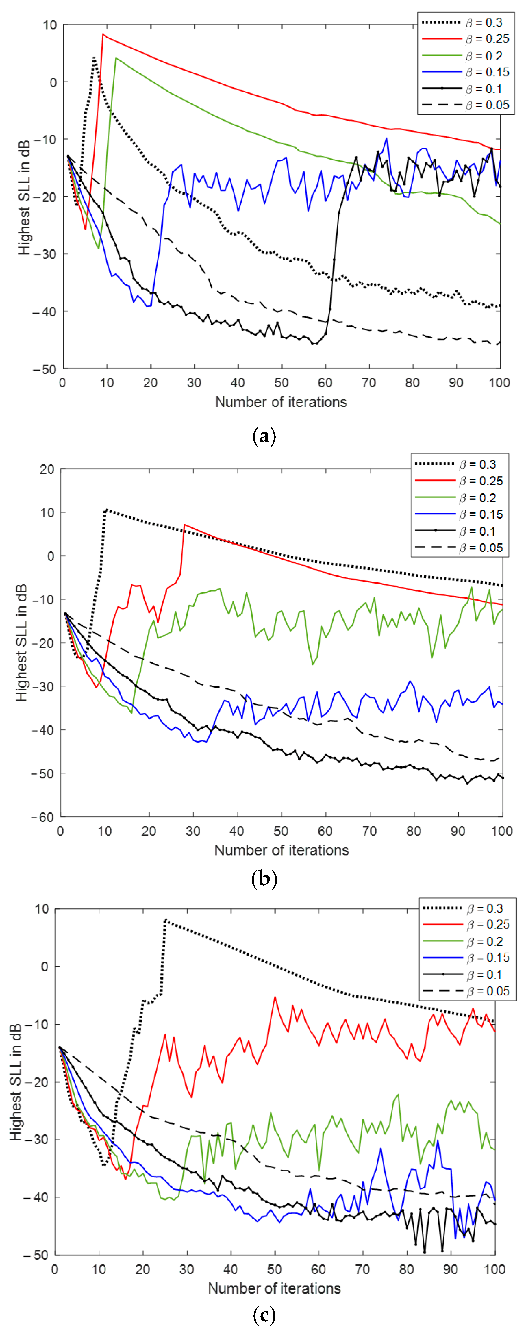
3.1. Performance of MPS Beamformer with the Convergence Control Factor β

The convergence control factor is one of the most important parameters for achieving the convergence towards deep SLL in MPS beamformer design. The cumulative addition of multibeams has some parasitic secondary sidelobes due to the multibeams sidelobes which may result in severe corruption in the overall array factor due to the divergence occurred in Equation (10). If β 1 , then the convergence is assured but with very slow rate while higher values of β leads to faster SLL reduction until a critical value at which divergence occurs. To examine the MPS beamformer performance with β , consider three different square array sizes of 10 × 10 , 20 × 20 and 30 × 30 elements using 48, 108 and 168 multibeams according to Equation (9), respectively, at α = 3 . The SLL learning curves at different values of β are shown in Figure 4 during 100 iterations, where divergence occurs at values of β greater than 0.1 especially when deep SLL below −45 dB are required. The performance of the MPS beamformer for the three array sizes has some consistent convergence properties especially the critical value of β at which divergence occurs and the speed of convergence where the values of β that are greater than 0.1 provide short convergence curves and provides limited deep SLL values. On the other hand, the learning behavior is stable at values of β < 0.1 , however it becomes slower due to the weak reduction in the SLL after each cycle. Therefore, there is a compromise between how deep the required SLL and the processing time. For most array sizes, SLL of −30 dB or less can be achieved faster by using β = 0.2 , while deep SLL values near −45 dB can be achieved at β 0.1 , so, the optimum value of β regarding processing speed depends on the required SLL and the array size.

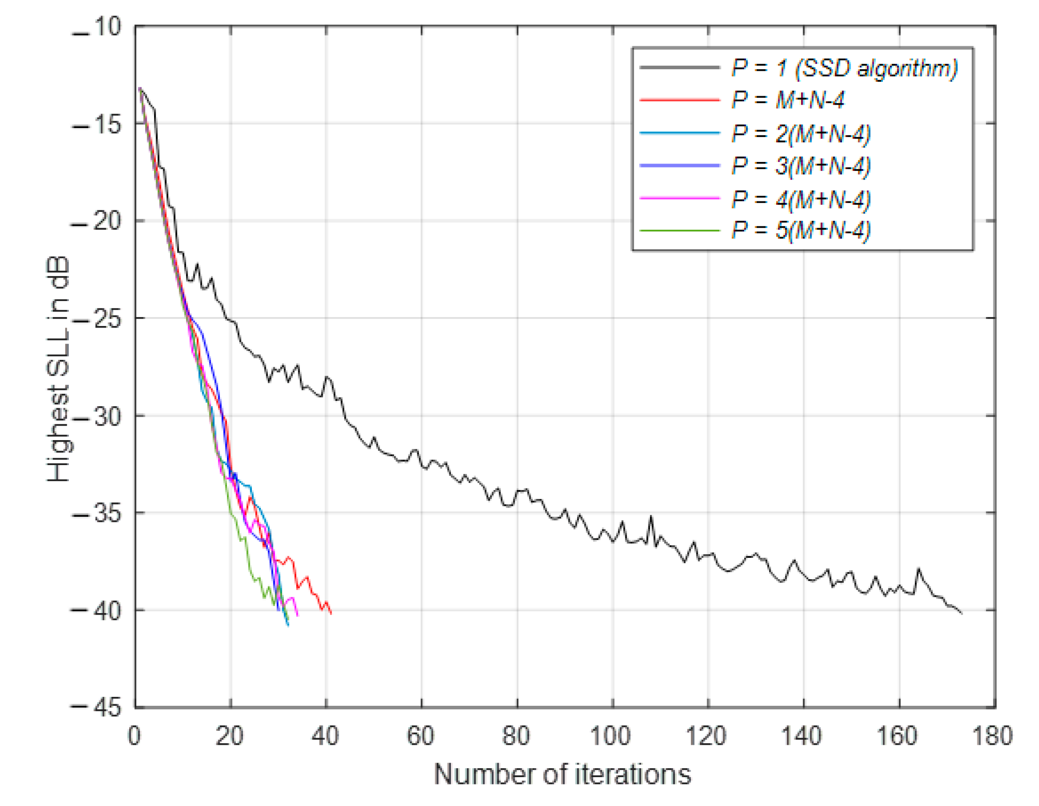
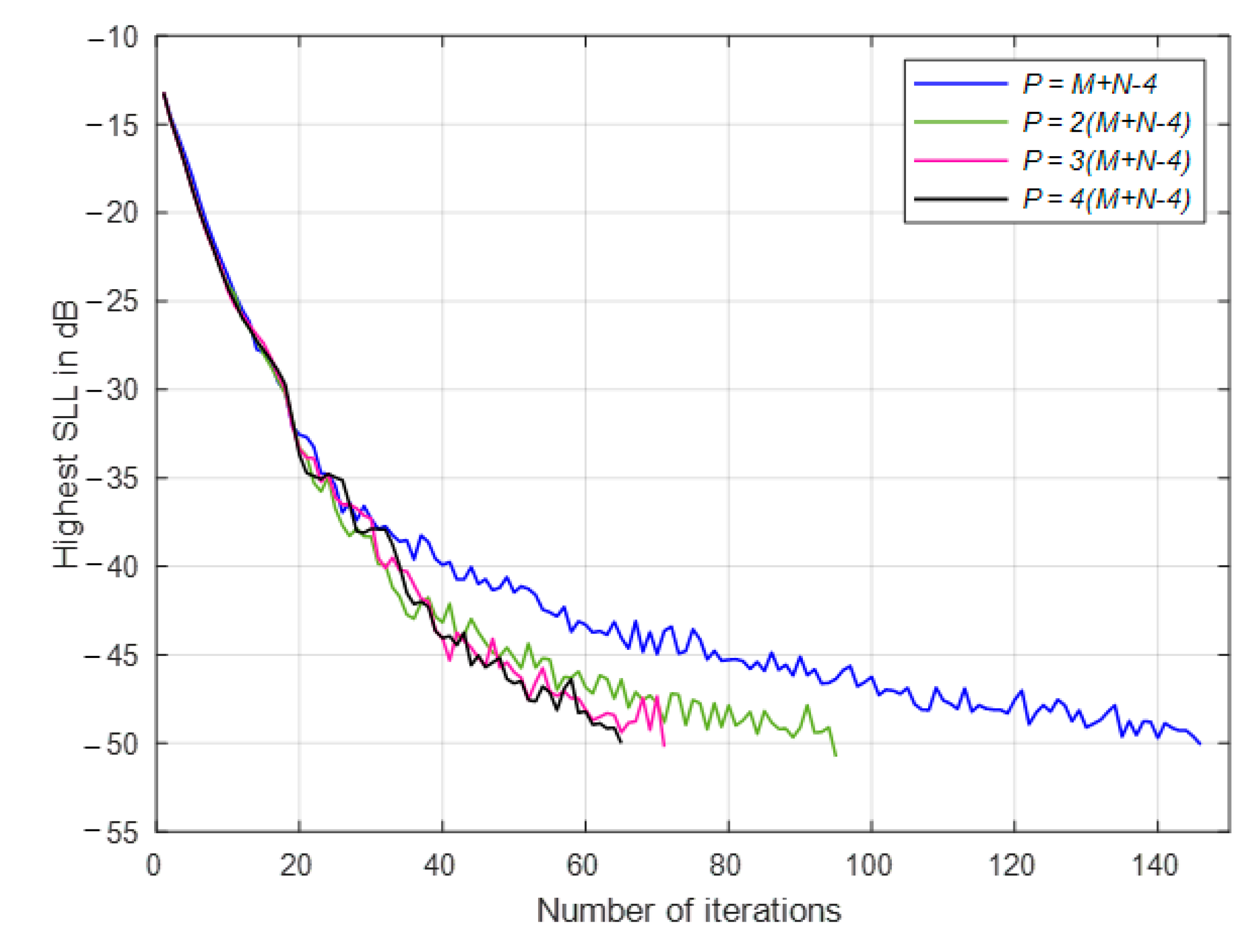
3.2. Performance of MPS Beamformer with the Number of Multibeams P

Adopting larger number of multibeams in Equation (9) is expected to reduce the processing time significantly in the MPS beamformer, however the divergence of the learning curve becomes faster also due to the cumulative addition of multibeams sidelobes especially at higher values of β as discussed in the previous section. To investigate this learning behavior, we examine the learning curves at different values of P as shown in Figure 5 for an array of 16 × 16 elements with β = 0.1 for the multibeam case while we use β = 0.7 for the single sidelobe sequential suppression as in [32] to speed up the convergence for that algorithm and for comparison purposes. The iteration cycles continue to achieve a −40 dB SLL at several values of P as shown in Figure 5 where there is a significant reduction in the required number of iterations in the MPS beamformer if we include larger number of multibeams in the reduction process. The single beam sidelobe sequential damping (SSD) algorithm [33] provides a stable convergence profile, however, it requires very large number of iterations to achieve deep SLL which is more than five times of that required in the MPS beamformer case although a higher value of β is used.
In terms of the absolute processing time in seconds, the comparison in Figure 5 has been conducted by a platform using i7-8550U CPU @ 1.80 GHz with 16 GB RAM. In addition, MATLAB 2021b is used in the simulation of the proposed MPS beamformer and the SSD algorithm as well. The average absolute processing time in seconds is shown Table 1 which is consistent with the data presented in Figure 5.
The performance of MPS beamformer at different number of multiple major sidelobes is almost the same at SLL values of −35 dB or higher, while there is a significant difference at lower SLL values as shown in Figure 6. Utilizing the first major sidelobes can provide deep SLL of −50 dB after 143 iterations while incorporating the second set of major sidelobes quickly achieve this level after approximately 95 iterations. Increasing the number of multibeams to include the third and fourth major sidelobes decreases the processing time where at P = 4 (M + N − 4) the required number of iterations is reduced to only 64 cycles. Any increase in P will not add any tangible performance improvement and it may requires decreasing the value of β to maintain convergence which in turn requires larger number of iterations. Therefore, including the first two to four major sidelobe groups is very sufficient for achieving deep SLL at lower processing time.

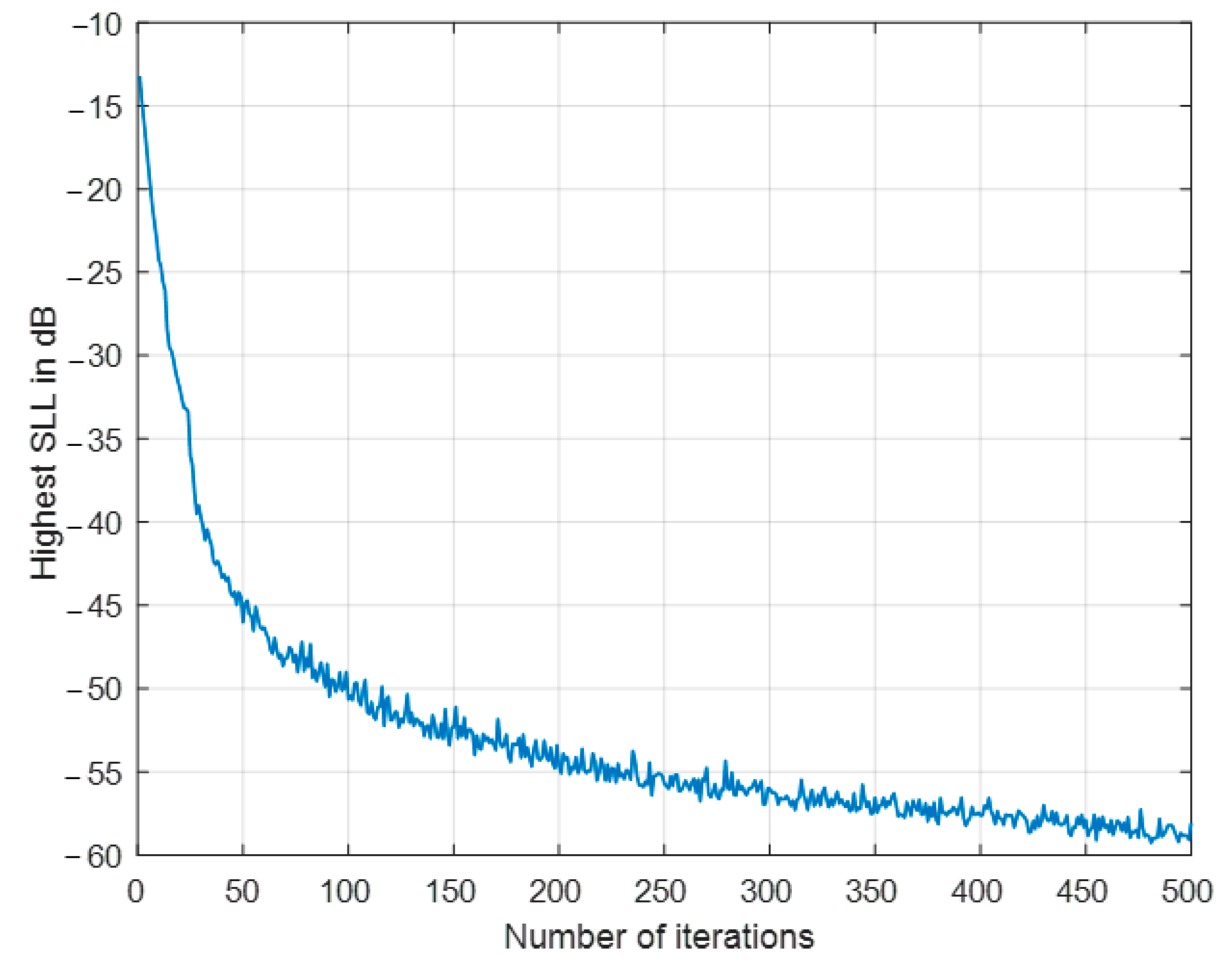
3.3. Performance of MPS Beamformer with the Number of Iterations I

As investigated in the previous section, increasing the number of multibeams in MPS beamformer is very important to speed up the SLL reduction process. On the other hand, for a specific number of multibeams, increasing the number of iterations provides deeper SLL at a decreasing exponential profile due to the increased number of almost near or equal sidelobes in the resulted radiation pattern. Figure 7 demonstrates the convergence profile versus number of iterations for an array of 16 × 16 elements with β = 0.1 using the first two major sidelobe groups (i.e., P = 2(M + N4)). From this figure, approximately 100 iteration cycles are required to achieve −50 dB while decreasing the required SLL to −60 dB requires more than 500 cycles.

3.4. Impact of Array Rounded Corners Structures on the MPS Beamformer Performance

The rounded corners planar arrays have the advantages of azimuth-independent beam scanning as well as lower sidelobe levels. These array designs have slightly different sidelobes patterns and distribution where they tend to be distributed in circular planes rather than perpendicular planes that exist in the square and rectangular arrays designs. Practically, and with uniform feeding, the rounded corners planar arrays have approximately a SLL of about −17 dB which is lower than the square or rectangular arrays by 2.5 dB. The rounded corners planar array can be optimized also using the MPS beamformer where the proposed algorithm is not sensitive to sidelobes distribution and, indeed, can be applied to any array design provided that the original array factor has identified sidelobe peaks to be nulled out. Figure 8a shows a rounded corner square array formed by trimming 8 elements at each corner by setting δ T = 0.8   δ M A X for a 16 × 16 square array. The normalized array factor is depicted in Figure 8b using uniform feeding where the sidelobes tend to be distributed circularly around the main lobe while the optimized normalized array factor to achieve −50 dB SLL is shown in Figure 8c after running 71 iterations using three major sidelobe groups with β = 0.1 as demonstrated in Figure 8d.

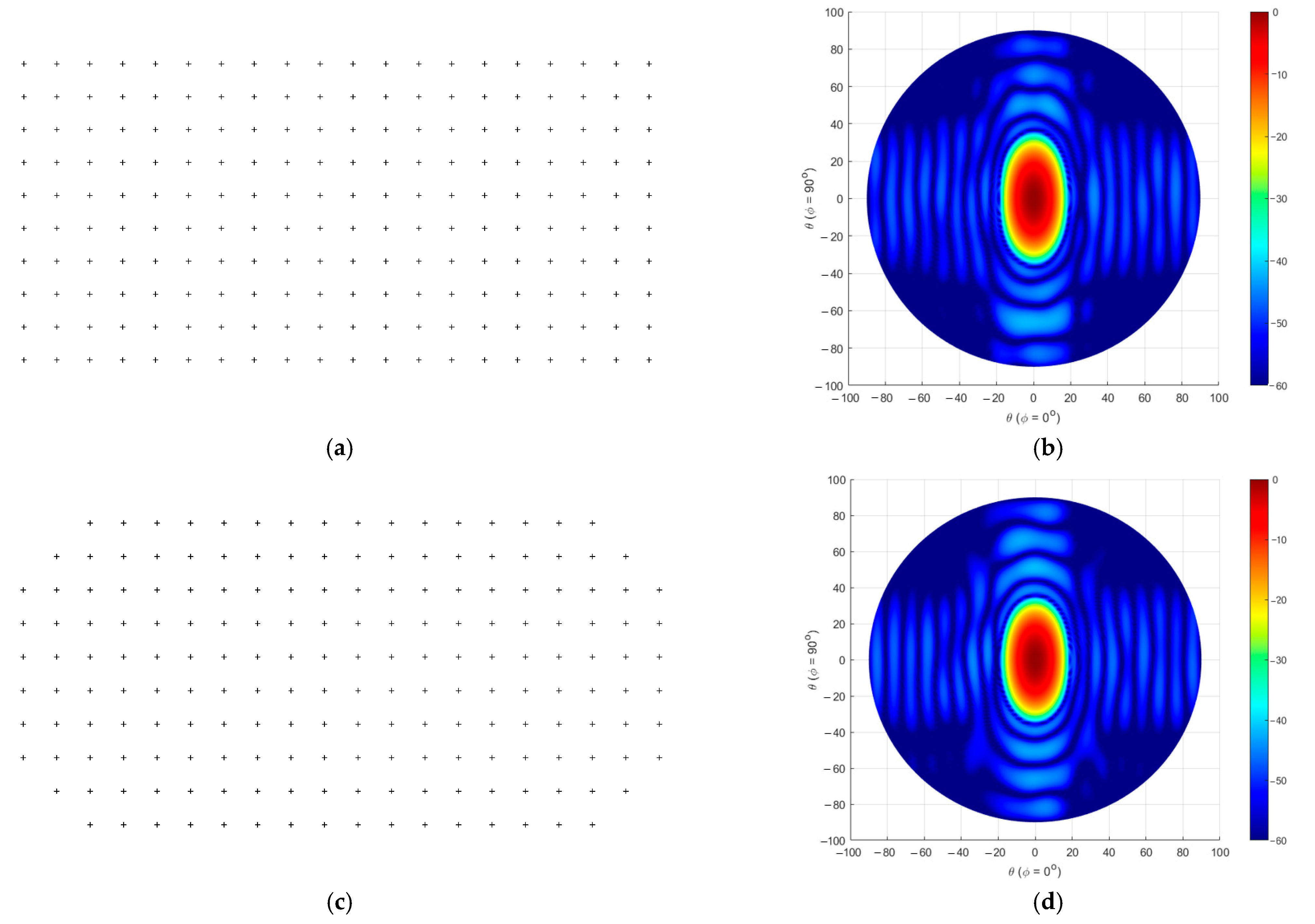
3.5. Performance of MPS Beamformer for Rectangular Arrays

As the MPS beamformer searches for the radiation peaks other than the mainlobe, it is expected to work with rectangular planar arrays also. Figure 9a,b display the configuration and optimized radiation pattern for a rectangular array of 1 0 × 20 elements using the first two major sidelobe planes (i.e., P = 2 (M + N4)) at β = 0.1 to achieve −45 dB SLL. The MPS beamformer converges to the required SLL with elliptic beam cross section due to the rectangular array configuration. The impact of rounded corners on the same optimized rectangular array has minimal effects as shown in Figure 9c,d for   δ T = 0.8   δ M A X where the reduced sidelobes have slightly spread over wider angular ranges.

3.6. Angular Scanning Performance of MPS Beamformer

The previous analysis of the MPS beamformer has been conducted for the case where the mainlobe direction is set at ( 0 ° , 0 ° ) to clearly identify the sidelobes in the radiation pattern. To optimize the array at any other mainlobe directions, we can utilize the same amplitude coefficients obtained at ( 0 ° , 0 ° ) and provide the necessary phase shifts for the new mainlobe direction as in phased arrays. However, the SLL should be at the required level so that the array weights optimization is carried out one time and should not repeated if the mainlobe is changed. According to Equation (10), the resulting overall weighting matrix after executing the algorithm for I iterations at the broadside mainlobe direction ( 0 ° , 0 ° ) is given by:
W o = S ( 0 ° , 0 ° ) β i = 1 I p = 1 P S U M ( A F i H ( θ p , ϕ p ) | N S ( θ p , ϕ p ) )
Therefore, the weighting matrix at any mainlobe direction ( θ o , ϕ o ) is given by the following phasing equation:
  W ( θ o , ϕ o ) = | W o | S ( θ o , ϕ o )
where | W o | is the absolute value of the coefficients of W o .
Figure 10a displays the amplitude coefficients for an array formed by 20 × 20 elements using the first two major sidelobe groups (i.e., P = 2(M + N − 4)) at β = 0.1 to achieve −40 dB SLL. The array weights in this figure exhibits tapered profile as expected for SLL reduction. Providing the proper phasing to this amplitude coefficients as in Equation (12) moves the mainlobe to the desired direction as shown in Figure 10b where the SLL remains at the same required level ( −40 dB). Therefore, the proposed MPS beamformer has consistent and solid performance with the varying mainlobe direction which simplifies the optimization process to be carried out only one time according to the required SLL. In Figure 10b, and for θ o 60 ° , the pattern has higher radiation levels near the array surface due to the array geometrical projection (reduced array effective area) which is known for all array planar structures, however the other side SLL values (towards the broadside direction) has the same required SLL even at directions near the endfire of the array (i.e., θ o = 90 ° ) which is very important for scanning beam applications such as in radar systems.

4. Comparison between MPS Beamformer and Conventional Tapering Windows

There are a lot of efficient amplitude windowing techniques that provides reduced SLLs for linear arrays which may be applied also to planar arrays. In this section, we will examine different efficient tapering windows such as squared cosine, Hamming, and Blackman windows [10] which are then compared with the proposed MPS beamformer. Consider a square array of 16 × 16 elements using the first major sidelobe planes (i.e., P = M + N − 4) at β = 0.1 to achieve −45 dB SLL using MPS beamformer. This array is also fed using the three comparison windows as shown in Figure 11 along with the reference uniform feeding case. The three compared tapered windows provide fixed SLL for each which cannot be adapted to lower values where the squared cosine and Hamming windows provides almost the same SLL of −21.7 dB while Blackman window provides an improved SLL of −32 dB. The proposed MPS beamformer provides deeper SLL according to the number of iterations at the price of increased beamwidth compared to the three tapered windows as investigated in Figure 11 where −45 dB or lower can be achieved. Therefore, the proposed MPS beamformer can be applied to achieve lower and controlled SLL which cannot be achieved by these efficient conventional windows for planar array structures. On the other hand, the achieved lower SLL level of the MPS beamformer is accompanied by some increase in the mainlobe beamwidth which can be overcome by increasing the array size.

5. Conclusions

The optimization of planar two-dimensional arrays has been achieved in this paper where the unwanted sidelobes are reduced using recursive multibeam pattern subtraction (MPS) algorithm. The proposed beamforming technique has been demonstrated and analyzed where the convergence to the desired maximum SLL is guaranteed by including control factor along with the proper number of multibeams in the reduction process. The adoption of multibeams in SLL reductions for planar arrays resulted in significant reduction in the processing time compared with the recent related techniques and can provide deeper SLL values relative to the conventional efficient tapered windows. In addition, the simulation results show that the MPS beamformer can operate with rounded corner structures as it depends on the presence of identified sidelobes in the original array radiation pattern. On the other hand, the optimization can be achieved only one time and the obtained amplitude weights can be applied at any other mainlobe direction after inserting the suitable phase shifts. In addition, the proposed MPS beamformer provides the same SLL over the whole angular ranges from broadside to endfire directions which is very important for beam scanning applications.

Author Contributions

Conceptualization, Y.A.; methodology, Y.A.; software, Y.A. and F.A.; validation, Y.A. and F.A.; formal analysis, Y.A.; investigation, F.A.; writing—original draft preparation, Y.A.; writing—review and editing, F.A. and Y.A.; visualization, Y.A.; funding acquisition, Y.A. All authors have read and agreed to the published version of the manuscript.

Funding

Taif University Researchers Supporting Project number (TURSP-2020/161), Taif University, Taif, Saudi Arabia.

Acknowledgments

The authors would like to thank Taif University Researchers Supporting Project number (TURSP-2020/161), Taif University, Taif, Saudi Arabia, for supporting this work.

Conflicts of Interest

The authors declare no conflict of interest.

References

  1. Akyildiz, I.F.; Nie, S.; Lin, S.-C.; Chandrasekaran, M. 5G roadmap: 10 key enabling technologies. Comput. Netw. 2016, 106, 17–48. [Google Scholar] [CrossRef]
  2. Artiga, X.; Perruisseau-Carrier, J.; Pérez-Neira, A.I. Antenna array configurations for massive MIMO outdoor base stations. In Proceedings of the 2014 IEEE 8th Sensor Array and Multichannel Signal Processing Workshop (SAM), A Coruna, Spain, 22–25 June 2014; pp. 281–284. [Google Scholar] [CrossRef]
  3. Amani, N.; Bencivenni, C.; Glazunov, A.A.; Ivashina, M.V.; Maaskant, R. MIMO channel capacity gains in mm-wave LOS systems with irregular sparse array antennas. In Proceedings of the 2017 IEEE-APS Topical Conference on Antennas and Propagation in Wireless Communications (APWC), Verona, Italy, 1–15 September 2017; pp. 264–265. [Google Scholar] [CrossRef] [Green Version]
  4. Pałczyński, K.; Śmigiel, S.; Gackowska, M.; Ledziński, D.; Bujnowski, S.; Lutowski, Z. IoT Application of Transfer Learning in Hybrid Artificial Intelligence Systems for Acute Lymphoblastic Leukemia Classification. Sensors 2021, 21, 8025. [Google Scholar] [CrossRef] [PubMed]
  5. Hasan, M.Z.; Al-Rizzo, H. Beamforming Optimization in Internet of Things Applications Using Robust Swarm Algorithm in Conjunction with Connectable and Collaborative Sensors. Sensors 2020, 20, 2048. [Google Scholar] [CrossRef] [Green Version]
  6. Cray, B.A.; Kirsteins, I. A Comparison of Optimal SONAR Array Amplitude Shading Coefficients. Acoustics 2019, 1, 808–815. [Google Scholar] [CrossRef] [Green Version]
  7. Li, J.; Ma, Z.; Mao, L.; Wang, Z.; Wang, Y.; Cai, H.; Chen, X. Broadband Generalized Sidelobe Canceler Beamforming Applied to Ultrasonic Imaging. Appl. Sci. 2020, 10, 1207. [Google Scholar] [CrossRef] [Green Version]
  8. Wang, Y.; Yang, W.; Chen, J.; Kuang, H.; Liu, W.; Li, C. Azimuth Sidelobes Suppression Using Multi-Azimuth Angle Synthetic Aperture Radar Images. Sensors 2019, 19, 2764. [Google Scholar] [CrossRef] [Green Version]
  9. Ruiz-de-Azua, J.A.; Garzaniti, N.; Golkar, A.; Calveras, A.; Camps, A. Towards Federated Satellite Systems and Internet of Satellites: The Federation Deployment Control Protocol. Remote Sens. 2021, 13, 982. [Google Scholar] [CrossRef]
  10. Prabhu, K.M.M. Window Functions and Their Applications in Signal Processing; Taylor & Francis: London, UK, 2014. [Google Scholar]
  11. Lau, B.K.; Leung, Y.H. A Dolph-Chebyshev approach to the synthesis of array patterns for uniform circular arrays. In Proceedings of the 2000 IEEE International Symposium on Circuits and Systems, Geneva, Switzerland, 28–31 May 2000; Volume 1, pp. 124–127. [Google Scholar]
  12. Dessouky, M.; Sharshar, H.; Albagory, Y. An Approach for Dolph-Chebyshev Uniform Concentric Circular Arrays. J. Electromagn. Waves Appl. 2007, 21, 781–794. [Google Scholar] [CrossRef]
  13. Aljahdali, S.; Nofal, M.; Albagory, Y. A modified array processing technique based on Kaiser window for concentric circular arrays. In Proceedings of the 2012 International Conference on Multimedia Computing and Systems, ICMCS 2012, Tangiers, Morocco, 10–12 May 2012. [Google Scholar]
  14. Almagboul, M.A.; Shu, F.; Qian, Y.; Zhou, X.; Wang, J.; Hu, J. Atom search optimization algorithm based hybrid antenna array receive beamforming to control sidelobe level and steering the null. AEU Int. J. Electron. Commun. 2019, 111, 152854. [Google Scholar] [CrossRef]
  15. Neroni, M. Ant Colony Optimization with Warm-Up. Algorithms 2021, 14, 295. [Google Scholar] [CrossRef]
  16. Sharaqa, A.; Dib, N. Circular antenna array synthesis using firefly algorithm. Int. J. RF Microw. Comput. Aided Eng. 2014, 24, 139–146. [Google Scholar]
  17. Chakravarthy, V.; Rao, P.M. Circular array antenna optimization with scanned and unscanned beams using novel particle swarm optimization. Indian J. Appl. Res. 2015, 5, 790–793. [Google Scholar]
  18. Meng, X.; Liu, Y.; Gao, X.; Zhang, H. A New Bio-inspired Algorithm: Chicken Swarm Optimization. In Advances in Swarm Intelligence; Tan, Y., Shi, Y., Coello, C.A.C., Eds.; ICSI: Lecture Notes in Computer Science; Springer: Cham, Switzerland, 2014; Volume 8794. [Google Scholar] [CrossRef]
  19. Singh, U.; Salgotra, R. Synthesis of linear antenna array using flower pollination algorithm. Neural Comput. Appl. 2018, 29, 435–445. [Google Scholar] [CrossRef]
  20. Saxena, P.; Kothari, A. Optimal Pattern Synthesis of Linear Antenna Array Using Grey Wolf Optimization Algorithm. Int. J. Antennas Propag. 2016, 2016, 1205970. [Google Scholar] [CrossRef] [Green Version]
  21. Mehrabian, A.; Lucas, C. A novel numerical optimization algorithm inspired from weed colonization. Ecol. Inform. 2006, 1, 355–366. [Google Scholar] [CrossRef]
  22. Sun, G.; Liu, Y.; Chen, Z.; Zhang, Y.; Wang, A.; Liang, S. Thinning of concentric circular antenna arrays using improved discrete cuckoo search algorithm. In Proceedings of the 2017 IEEE Wireless Communications and Networking Conference (WCNC), San Francisco, CA, USA, 19–22 March 2017; pp. 1–6. [Google Scholar]
  23. Li, H.; Liu, Y.; Sun, G.; Wang, A.; Liang, S. Beam pattern synthesis based on improved biogeography-based optimization for reducing sidelobe level. Comput. Electr. Eng. 2017, 60, 161–174. [Google Scholar] [CrossRef]
  24. Van Luyen, T.; Giang, T.V.B. Interference Suppression of ULA Antennas by Phase-Only Control Using Bat Algorithm. IEEE Antennas Wirel. Propag. Lett. 2017, 16, 3038–3042. [Google Scholar] [CrossRef]
  25. Mirjalili, S.; Lewis, A. The Whale Optimization Algorithm. Adv. Eng. Softw. 2016, 95, 51–67. [Google Scholar] [CrossRef]
  26. Liang, S.; Fang, Z.; Sun, G.; Liu, Y.; Qu, G.; Zhang, Y. Sidelobe Reductions of Antenna Arrays via an Improved Chicken Swarm Optimization Approach. IEEE Access 2020, 8, 37664–37683. [Google Scholar] [CrossRef]
  27. Sun, G.; Liu, Y.; Li, H.; Liang, S.; Wang, A.; Li, B. An Antenna Array Sidelobe Level Reduction Approach through Invasive Weed Optimization. Int. J. Antennas Propag. 2018, 2018, 4867851. [Google Scholar] [CrossRef] [Green Version]
  28. Wei, T.; Wang, S.; Zhong, J.; Liu, D.; Zhang, J. A Review on Evolutionary Multi-Task Optimization: Trends and Challenges. IEEE Trans. Evol. Comput. 2021, 1. [Google Scholar] [CrossRef]
  29. Sahalos, J.N. Design of shared aperture radar arrays with minimum sidelobe level of the two-way array factor. IEEE Trans. Antennas Propag. 2020, 68, 5415–5420. [Google Scholar]
  30. Parker, M. Digital Signal Processing 101; Elsevier: Amsterdam, The Netherlands, 2010; pp. 201–211. ISBN 9781856179218. [Google Scholar] [CrossRef]
  31. Gangwar, V.S.; Singh, A.K.; Singh, S.P. An Effective Approach for the Synthesis of Unequally Spaced Antenna Array by Estimating Optimum Elements Density on the Aperture. IEEE Antennas Wirel. Propag. Lett. 2017, 16, 2278–2282. [Google Scholar] [CrossRef]
  32. Albagory, Y.; Alraddady, F. An Efficient Approach for Sidelobe Level Reduction Based on Recursive Sequential Damping. Symmetry 2021, 13, 480. [Google Scholar] [CrossRef]
  33. Albagory, Y. An Efficient Fast and Convergence-Controlled Algorithm for Sidelobes Simultaneous Reduction (SSR) and Spatial Filtering. Electronics 2021, 10, 1071. [Google Scholar] [CrossRef]
  34. Albagory, Y.; Alraddady, F. An Efficient Adaptive and Steep-Convergent Sidelobes Simultaneous Reduction Algorithm for Massive Linear Arrays. Electronics 2022, 11, 170. [Google Scholar] [CrossRef]
Figure 1. Planar two-dimensional array formed by M × N isotropic elements in the XY-plane.
Electronics 11 01015 g001
Figure 2. Normalized power gain in dB of a broadside beam originating from 16 × 16 planar array with uniform feeding.
Electronics 11 01015 g002
Figure 3. Subtracted multibeam and the resulting array normalized power patterns in dB, respectively: (a,b) after one reduction cycle, (c,d) after 16 reduction cycles, and (e,f) after 68 reduction cycles.
Electronics 11 01015 g003aElectronics 11 01015 g003b
Figure 4. MPS beamformer learning curves variation with the number of iterations of reduction at different values of β and for array sizes: (a) 10 × 10 , (b) 20 × 20 , and (c) 30 × 30 .
Electronics 11 01015 g004
Figure 5. Convergence profiles at different number of subtracted multibeams.
Electronics 11 01015 g005
Figure 6. MPS beamformer convergence profiles at different number of subtracted multibeams.
Electronics 11 01015 g006
Figure 7. MPS beamformer SLL reduction profile with the number of iterations.
Electronics 11 01015 g007
Figure 8. MPS beamformer performance for rounded-corners planar arrays: (a) array structure, (b) normalized array power gain for the uniform feeding case in dB, (c) normalized array power gain after 71 iterations to achieve −50 dB SLL, and (d) the convergence profile of the MPS beamformer to achieve the SLL in (c).
Electronics 11 01015 g008
Figure 9. MPS beamformer performance for rectangular planar arrays: (a) array structure of 10 × 20 elements (b) normalized array power gain in dB to achieve −45 dB SLL, (c) the rounded-corners rectangular array structure at δ T = 0.8   δ M A X , and (d) normalized array power gain in dB to achieve −45 dB SLL for the array in (c).
Electronics 11 01015 g009
Figure 10. The MPS beamformer scanning performance for 20 × 20 array optimized to achieve SLL of −40 dB: (a) normalized element coefficient amplitude and (b) normalized array power gain of the scanning beam at different values of θ o .
Electronics 11 01015 g010
Figure 11. Normalized array power pattern comparison between the MPS beamformer and tapered windows.
Electronics 11 01015 g011
Table 1. Average processing time required for achieving −40 dB SLL using the MPS beamformer at different number of multibeams and SSD algorithm in [32].
Number of MultibeamsAverage Processing Time in Seconds
Single beam (SSD Algorithm in [32])469.59
M + N 4 105.1
2 ( M + N 4 ) 78.0
3 ( M + N 4 ) 86.5
4 ( M + N 4 ) 88.0
5 ( M + N 4 ) 86.6
Publisher’s Note: MDPI stays neutral with regard to jurisdictional claims in published maps and institutional affiliations.

