1. Introduction
The Gough–Stewart (G-S) platform had been extensively employed as a motion base for flight simulators [
1], which will provide high-fidelity motion cueing for pilot training when combined with a visual system and audio system in the cockpit simulator. The theoretical advantages of the parallel structure heavily depend on its motion control strategy. Although an independent PI joint controller in joint space can be applied to the G-S platform motion system, it does not always guarantee high performance due to the strong coupling and high nonlinearity of the dynamic model [
2]. A cross-coupling control scheme was designed to solve the synchronization problem of the G-S platform with an adaptive feedforward gravity compensation [
3].
The high level of performance has to be guaranteed through model-based control strategies on the workspace, such as inverse dynamic control, adaptive control, sliding mode control, incremental nonlinear dynamic inversion control, etc. It is well known that the inverse dynamic control strategy in [
4] heavily depended on the exact modeling of the complete G-S dynamic model, which would inevitably lead to a high computational burden. Meanwhile, the study in [
5] showed that the control strategy based on a simplified model provided better tracking performance than those based on a complete dynamic model.
In addition, due to the fact that the G-S motion systems suffered from parameter uncertainties and unmodeled uncertainties, more advanced model-based control strategies such as adaptive control, robust control, and sliding mode control are necessary. The adaptive control scheme is restricted to simple parallel mechanisms [
6,
7] or a strongly simplified G-S dynamic model [
8] due to the complicated linear form of the complete dynamic model. The robust control scheme provided another way to deal with model uncertainties and had been employed for a six-degrees-of-freedom (DOF) parallel manipulator [
9,
10]. The sliding mode control is another well-studied control scheme to enhance motion system robustness [
11,
12,
13,
14]. In addition, other model-based control [
15], isotropic control [
16], or incremental nonlinear dynamic inversion control [
17] were proposed to enhance the motion tracking performance of the G-S platform.
As for control schemes designed for a six-DOF spatial rigid body, those conventional control schemes based on local motion parameterization for limited motion ranges cannot be applied to rigid body systems with large range of motion [
18]. In order to model a six-DOF spatial rigid body in a geometric framework, the configuration (position and orientation) of a rigid body is represented globally on a six-dimensional special Euclidean space SE(3) in a coordinate-free manner. The nonlinear control problems whose configurations are defined on Lie group space have received considerable attention in the recent literature. The early remarkable contributions from Brockett’s research mainly focused on controllability issues [
19]. Generally, there exist two geometric frameworks to define the configuration error on SE(3). One is related to exponential coordinates on Lie group SE(3) [
20,
21,
22], and another one is expressed with left or right group operation between the current configuration and desired configuration [
23]. Their velocity errors were calculated with the adjoint operator in its Lie algebra tangent space. With these kinematic state error vectors expressed in the Lie group and Lie algebra space, some controllers that were directly designed on SE(3) were provided, and their closed-loop stability was also verified. Bullo focused on exploiting the geometric structure of Lie groups and generalizing the classical PD feedback used for the control of simple mechanical systems in
[
20,
23]. With the configuration error vector based on exponential coordinates on SE(3), Lee proposed a robust adaptive terminal sliding mode control strategy [
24,
25], while Jiang designed an asymptotic law for the spacecraft hovering over an asteroid with the second-order derivative of exponential coordinates [
26]. Furthermore, Wang put forward another new configuration error function to design a geometric terminal sliding mode controller on SE(3) [
27].
In the flight simulator application, the contribution of its cockpit payload mounted at the upper moving platform is much more significant than the six legs in dynamic modeling of the six-DOF spatial G-S motion platform due to its limited motion envelope. Thus, the dynamic model component related with leg movement can be considered as bounded time-varying model uncertainty so as to take the control problem of the G-S platform as a control problem of the rigid body system defined on the Lie group SE(3) with bounded model uncertainty. In addition, acceleration instead of positional accuracy is much more critical for flight simulation motion systems. This gives us the motivation to develop a robust terminal sliding mode controller on SE(3) to provide robustness to counteract imperfect compensation due to its model simplification and payload parameter uncertainties for the flight simulator motion platform. Meanwhile, as pointed out in [
10], in order to reduce the computation time, the inertial matrix and Coriolis matrix of conventional robust control law can be approximated as constants that define at the neutral point without introducing large modeling errors. Hence, the model-based robust control strategy on Cartesian space had to provide robustness to overcome this imperfect configuration-dependent model simplification uncertainty in addition to payload parameter uncertainty. However, the TSMC on Lie group SE(3) does not need to consider this configuration-dependent uncertainty, as the inertial matrix of the upper platform was constant when the kinematic state is expressed in the upper moving platform-fixed coordinate. Thus, the TSMC on SE(3) is expected to provide better robustness than TSMC on Cartesian space. It is designed to guarantee almost global finite-time convergence through the Lyapunov stability theory. Therefore, the main contribution of this work can be summarized as follows:
The outline of this paper is listed as follows. In
Section 2, a mathematical complete dynamic model of the G-S platform in geometric mechanics is derived with its kinematic state expressed in the moving platform-fixed coordinate frame. Meanwhile, a corresponding G-S computer model that was built with the Simcape module from the MATLAB/Simulink package is taken as a forward dynamic model. With exponential coordinate for configuration error and adjoint operator for velocity error, a robust terminal sliding mode controller on SE(3) is designed through the Lyapunov stability analysis in
Section 3. Given the description of two standard tests (the describing function, step acceleration response) and numerical experimental setup, the proposed TSMC strategy on SE(3) is verified and compared with the conventional TSMC strategy on Cartesian space in
Section 4. Finally, the conclusions are drawn in
Section 5.
2. Dynamic Models of Gough-Stewart Platform
In this section, we will first provide a complete mathematical dynamic model of the G-S motion platform system in the body-fixed kinematic state, which preserves the geometric mechanical structure of the upper moving platform. In addition, a computer model based on the Simscape module from the MATLAB/Simulink package is built as a forward dynamic model and has been verified with its mathematical model.
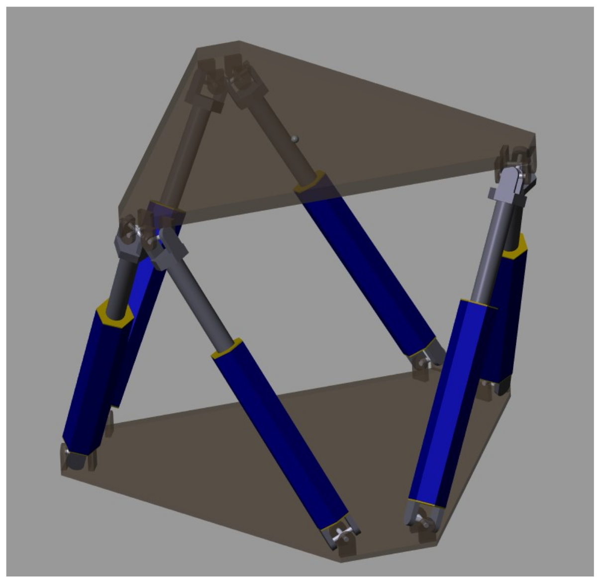
The geometric structure of a general G-S motion platform is shown in
Figure 1. One inertial coordinate frame
is fixed on the lower fixed platform, and one body frame
is fixed on the upper moving platform. Let
denote the configuration pose of the upper moving platform, which belongs to a special Euclidean group space
.
can be expressed with a
homogeneous matrix as follows,
Here,
is the translational vector of geometric center
of the upper moving platform described in the lower fixed frame
. R is the orientation matrix between these two coordinate frames, which can be parameterized by three Euler angles
in Z–Y–X order (Yaw–Pitch–Roll). Therefore, the configuration pose
can be locally parameterized through a six-dimensional Cartesian coordinate vector
. In order to exploit the geometric structure of the G-S dynamic model for the following controller design, we transform the Cartesian coordinate velocity
in frame
into body velocity
expressed in moving platform frame
,
where
is the transformation matrix between the body angular velocity
and Euler angle derivatives
.
As the upper moving platform contributes to the major part of the G-S complete dynamic model, especially when the ratio of the platform to the leg is obviously large, we can derive a complete dynamic model among which we can preserve the geometric mechanics of the upper moving platform.
where
denotes the inertia tensor matrix for the moving platform with payload,
is the gravity component vector for the moving platform payload,
is the gravity component of six legs, and
denotes the other residual component vector due to leg movement. Here,
denotes the kinematic Jacobian matrix with respect to new kinematic state
. The six-dimensional vector
is the actuator force that drives the six legs.
Here, is the moment of inertial parameters of the moving platform (including payload) in frame , is the mass parameters of the moving platform (including payload), is the CoG positional vector of the moving platform with its cockpit payload, which is expressed in the body-fixed frame . The operator is defined so that for all . The vector g is the constant gravitational acceleration.
The kinematic Jacobian matrix
and co-adjoint operator
are formulated as follows. The co-adjoint operator is applied to derive the dual of the Lie algebra.
where
denote link vectors of six legs expressed in the lower fixed frame
(see
Figure 1).
are the position vectors of six lower joints in the lower frame
, and
are the lengths of six links.
In addition, we also need to construct a forward dynamic model of the G-S motion platform as a controlled system plant. As a Simscape Multibody-based dynamic model is more insensitive to the floating-point calculation error, it is chosen as the forward dynamic simulation for the G-S platform motion system instead of its mathematical model. In this work, we modify the G-S example model in the Simscape Multibody Library with our custom parameters to construct an integrated simulation environment for controller performance evaluation. The Simscape model structure for the whole G-S platform and its 3D animation is shown in the following
Figure 2 and
Figure 3, respectively. Each leg model in
Figure 4 is composed of two universal joints connected to the upper and lower platform base, one extensive piston at the upper part of this leg and another one rotating cylinder at the lower part, while a two-DOF cylindrical joint connects the upper part and lower part of this leg.
Finally, a mutual inverse dynamic model output verification experiment between the mathematical model and Simscape-based computer model had been carried out by comparing the actuator force output when given the same trajectory for these two G-S models.
3. Robust Controller Design on Lie Group Space SE(3)
Recently, Lee had provided a robust adaptive terminal sliding mode control on SE(3) in the framework of geometric mechanics for the autonomous rendezvous and docking of two spacecraft with unknown disturbances and moment of inertia uncertainty [
24]. Inspired by this control scheme, we propose a TSMC strategy on SE(3) for the G-S motion platform to deal with fast-varying yet bounded model uncertainties due to model simplification as well as bounded slow-varying payload parameter variation. The control objective is to design control input such that the trajectory errors converge to zero asymptotically in finite time.
For a general G-S motion system, let
SE(3) be the desired configuration pose and
SE(3) be the current configuration pose. Thus, a natural configuration tracking error between
and
on Lie group space SE(3) can be defined with the right group operation as follows.
In this work, the configuration tracking error of the G-S platform can be further expressed in exponential coordinates using the following logarithm map,
where
is the logarithm map that maps a group element in SE(3) space to Lie algebra space
. We can regard the logarithmic map as a local chart of the manifold group SE(3) (more details can be seen in [
20]). Thus, the configuration tracking error is expressed in vector form of exponential coordinates as follows,
where
and
are exponential coordinate vectors for the attitude tracking error (principal rotation vector) and position tracking error, respectively. We should notice that the logarithm map is bijective when the principal angle of rotation has a magnitude less than
radians, i.e.,
.
The velocity error
between the current velocity
and desired velocity
can be derived in the Lie algebra vector space as follows,
where
is adjoint action on SE(3) that is defined as follows,
As given in reference [
20], the kinematics of exponential coordinates provided the relations between
and velocity error
as follows,
The explicit expansion formulation for matrix
can be found in [
20].
The time derivative of the velocity error
can be derived as follows,
where
is the Lie bracket operator for the Lie algebra vector (see Lie bracket definition in [
28]).
Substituting the acceleration Equation (12) to the G-S platform dynamic, Equation (3) produces the following configuration error dynamic equation,
where
is a composition for the gravity component of the moving platform and legs.
In flight simulation application, the characteristic of the G-S dynamic model depends on the commanded trajectory that provides high-quality motion cues for flight training. For example, in low-frequency motion, the actuators’ position and velocity constraint limit the maximal available acceleration. Moreover, the high-frequency motion keeps the moving platform not far away from its neutral position. Thus, the imperfect compensation due to model simplification also depends on its motion envelope for flight simulation.
As for the model simplification strategy, when a G-S dynamic model in Cartesian coordinate
q (see reference [
1]) was employed in model-based controller law for flight simulator application, the matrices
,
, and
need to be considered approximated as constant components with acceptable modeling errors. Under its motion envelope, the configuration pose-dependent inertial matrix for the upper moving platform with payload
could present
variation of its nominal inertial matrix at neutral pose in the low-frequency high-amplitude motion, contributing to
of the whole model simplification error. However, the model simplification based on dynamic model Equation (3) with configuration-independent inertial matrix
only presents model simplification error related to leg movement. For the leg part of both of these two dynamic models, its gravity component
and residual component
can be considered as a constant vector without generating large modeling errors under the limited motion envelope.
In addition, there are always slow time-varying or unknown parameter uncertainties for the upper platform with a changeable payload due to pilot adjustment or additional equipment. Therefore, both model simplification error and payload parameter uncertainties contribute to the G-S model uncertainties boundedness in the following Assumption 1. Based on this model simplification scheme and uncertainty boundedness, the derivation of model-based robust control law becomes much simpler, which would reduce the computation time significantly.
Assumption 1. (G-S Motion System imperfect model compensation boundedness) The simplified G-S dynamic model provided in Equation (3) contains imperfect model compensation from the intentional simplification of the leg component and inaccurate constant and time-varying model parameters. The generalized forces and torques corresponding to model error are assumed to be bounded. Thus, it is assumed that there exists a constant boundary vector such that It is obvious that the G-S model uncertainty in Equation (3) does not need to deal with configuration-dependent uncertainty related to a moving platform so as to provide us with a more reasonable boundary to enhance the robustness of the control law. The sliding mode control scheme is capable of dealing with model uncertainties. It is well known that a fundamental difference in flight simulator motion systems w.r.t usual robotics is the fact that acceleration instead of positional accuracy is more important. Thus, this work is devoted to designing a robust terminal sliding mode control scheme for the G-S motion system with model uncertainties.
The terminal sliding plane on the Lie group SE(3) is defined as follows,
where
is the sliding plane,
,
is a positive definite matrix, and the positive odd integers
are chosen such that
.
Theorem 1. For the nonlinear error kinematics and dynamics described in Equations (11) and (13), if the sliding plane is designed as Equation (15), the system motion will converge to zero along the sliding plane in finite time, and the control law is designed as follows,where , are saturation functions, and is a positive definite gain matrix satisfying the following inequality, Proof. Consider the following Laypunov function candidate,
Taking the time derivative of the Laypunov function
V results in,
Substituting the error dynamic Equation (13) and kinematic Equation (11) into Equation (19), the derivative will be written as,
Finally, taking the control law Equation (16) into Equation (20) yields the following equation.
where
and
is the minimum eigenvalue of inertia matrix
. Therefore, through the finite-time stability theorem in [
29], we can draw the conclusion that the G-S platform kinematic state will reach the sliding surface
in finite time. The closed-loop system under control law (16) will globally stabilize
in finite time. □
Remark 1. As mentioned in [30], in order to avoid the possible singularity problem in the TSMC as η converges to zero, the parameters p and q are properly chosen so that . The controller framework for the G-S motion system is shown in
Figure 5. Those six legs are actuated through a PMSM drive modeled through a simplified transfer function as clarified in reference [
12], and it can meet the controller demand output with a current loop bandwidth over 100 Hz in torque control mode. The forward kinematics of the G-S platform can be computed in real time by employing a Newton–Raphson method.
4. Controller Performance Evaluation and Analysis
This section is devoted to evaluating the robustness performance of the TSMC strategy on SE(3) through a comparison with the conventional TSMC strategy on Cartesian space in a G-S motion platform simulated testbed. The main parameters of the G-S motion system are shown in
Table 1 and
Table 2. In this work, two standard methods from the AGARD report 144 [
31] are considered: the describing function test for frequency domain evaluation and the step acceleration response for time domain evaluation. For each degree of freedom, six describing functions can be calculated at operating points in the following
Table 3. The primary describing function is the comparison of the response of motion base in the driven DOF to the excitation signal. The amplitudes of sinusoidal input were chosen to keep the motion below approximately
of the system limits in position, velocity, and acceleration. The amplitude of the step acceleration input is chosen to be
of the system limits. The simulation step size is chosen to be 0.01 ms, and the ODE45 solver is used.
For the Simscape-based G-S platform model plant, the parameter uncertainties of its moving platform payload are set with the following equations.
These payload parameter uncertainty equations show that the actual payload parameters vary in the range of 6–8% of its nominal values, which include a constant uncertainty and a slow time-varying uncertainty. With the known dynamic model simplification characteristic of G-S dynamics under a limited motion envelope, it is easy to determine a conservative boundary vector for a flight simulator motion system. Therefore, the controller parameters for TSMC on SE(3) are set as shown in
Table 4.
After the description of the test procedure and experimental setup, the amplitude and phase frequency characteristics of the closed-loop G-S motion system under the TSMC controller law on SE(3) from 0.3 to 20 Hz are shown in
Figure 6 and
Figure 7. Meanwhile, given the same describing function test and experimental setup, a TSMC strategy in Cartesian space provides the amplitude and phase frequency characteristics in the following
Figure 8 and
Figure 9.
For the TSMC strategy on SE(3), it can be seen that the systems presented a flat response with a bandwidth of approximately 20 Hz in the surge, sway, roll, pitch, and yaw directions. Meanwhile, the dB point of heave direction can be found around 13 Hz. In all six DOFs, the phase lag remains well within . However, for the TSMC strategy on Cartesian space, it is only in the surge, sway, roll, and yaw directions that the bandwidth can arrive at 20 Hz. In the heave direction, the dB point has dropped to 7.1 Hz. In the pitch direction, the dB point also falls to below 10 Hz, and the phase lag has exceeded around 15 Hz. Thus, we can draw the conclusion that the TSMC strategy on SE(3) provides better robustness with high bandwidth in two DOFs more than TSMC on Cartesian space.
Furthermore, given another set of controller parameters for the step acceleration response test (
,
, other parameters remain unchanged), the rise time comparisons in six DOFs are shown in
Table 5. This comparison shows that the TSMC on SE(3) represents a relatively faster step response than TSMC on Cartesian space in all six DOFs, especially in the roll and yaw direction. The acceleration step responses in the roll and yaw direction are shown in the following
Figure 10 and
Figure 11, respectively. It tells us that the TSMC on SE(3) also behaves with smaller acceleration tracking error than TSMC on Cartesian space. This is due to the fact that the TSMC strategy had to cost much more robustness in dealing with its configuration-dependent model simplification error in the high-amplitude rotation motion.
As stated by Koekebakker [
1], the controlled simulator motion system requires a bandwidth over 10 Hz so as to have minimal influence on the pilot–aircraft model loop characteristics. Through the performance comparison in the frequency-domain and time-domain, we can conclude that the TSMC strategy on SE(3) would be beneficial for robust controller design for a flight simulator motion base. In addition, it should be noticed that the frequency-domain and time-domain performance of the controlled system would worsen in physical implementation due to the increased response time of inner-loop PMSM drive systems.


