Article

Distributed Online Risk Assessment in the National Cyberspace

by
Andrzej Karbowski
Research and Academic Computer Network NASK—National Research Institute, ul. Kolska 12, 01-045 Warsaw, Poland
Electronics 2022, 11(5), 741; https://doi.org/10.3390/electronics11050741
Submission received: 31 December 2021 / Revised: 10 February 2022 / Accepted: 21 February 2022 / Published: 28 February 2022
(This article belongs to the Special Issue New Challenges on Cyber Threat Intelligence)

Abstract

:
The paper presents a distributed approach to online cyber risk assessment across the country, taking into account cyber threats and vulnerabilities identified by local services operators. It consists in distributed, asynchronous calculations of possible failure scenarios. They are a solution of a set of nonlinear, nonsmooth equations with locally assessed risk activation functions as inputs. These functions indicate whether a given threat is expected in some future period. The convergence condition of the mentioned algorithm is given in the theorem form. At the end, a case study concerning a system consisting of four entities is presented.

1. Introduction

The COVID-19 pandemic, during which many people started to work, learn, and study from home, has shown how important distributed systems are. It concerns especially clouds, their stability and reliability [1]. Microsoft TEAMS, Google Meet, and Zoom saw a very big increase of new people signing into them [1]. The importance of digital services has increased rapidly. Unfortunately, in this time of crisis, cyber criminals have become hyperactive and have been constantly preying on the sensitive data of both individual users and organizations. Because of that, cyber security needs to be upgraded to protect users against rising cyber crimes [2,3].
The distributed nature of the system implies that the underlying security controls and monitoring facilities should be also distributed, with the ability to apply filtering to minimize the exchange of information concerning security with the central node [4].
An alternative is a hierarchical approach: coordinator–local units, or master–workers, where there exists an entity responsible for national-level risk assessment—the Operations Center (CNT) and local entities (LE)—essential services operators, presented in the previous papers [5,6]. In such a system, local units participating in the calculations do not exchange information related to the risk assessment process for the whole or a part of the system; rather, they send data to the CNT after making their assessments.
A hierarchical approach can be embarrassing when a large amount of information is transferred to the CNT and when there are problems with connectivity to part of the system as a result of an attacker’s success. Moreover, when the CNT serves only to gather the data, calculate some aggregated values, and broadcast the results, the question arises whether the coordination is really necessary.
Therefore, it appears that a peer-to-peer system, closely related to the network topology, where different units perform calculations and exchange information with the direct neighbors [7,8,9], seems to be more appropriate.
The literature on the different approaches to dynamic risk assessment in critical infrastructure, including core IT systems, is very broad [10,11]. However, the models used for online calculations of possible event scenarios, based e.g., on attack graphs [12,13,14,15], system dynamics [16], Bayesian networks [17], and Markov chains [18,19], assume centralized processing. Just recently, an interesting decentralized model based on fuzzy Bayesian Games, looking for a consensus via delegated proof of stake (DPoS) and proof of work (PoW) algorithms was presented [20]. However, it was designed for multimicrogrid systems and uses the adequate low-level information.
The model presented here is the next step to work out a practical mechanism which is [21] “scenario-based, where actors are gathered together to consider scenarios in the round; such scenarios describe risks as a narrative and label them by applying simple categories of likelihood and impact”. However, unlike in references [5,6], likelihood does not have to take values from the interval [ 0 ,   1 ] (in some models it is more convenient to scale it to a different interval, e.g., [ 0 ,   100 ] ) and it is assumed that the influence of the neighbouring nodes is limited. The equations presented here are a little similar to those of studies [22,23,24] but they are nonlinear with saturation functions. In this paper, first such a model is presented in a detailed way, then the theorem concerning the convergence of the proposed iterative algorithm is formulated and proved. Finally, a case study concerning a system built from a power plant, a hospital, a railway operator, and a data center shows a scenario, that is the course of possible events, after an attack on the power plant.

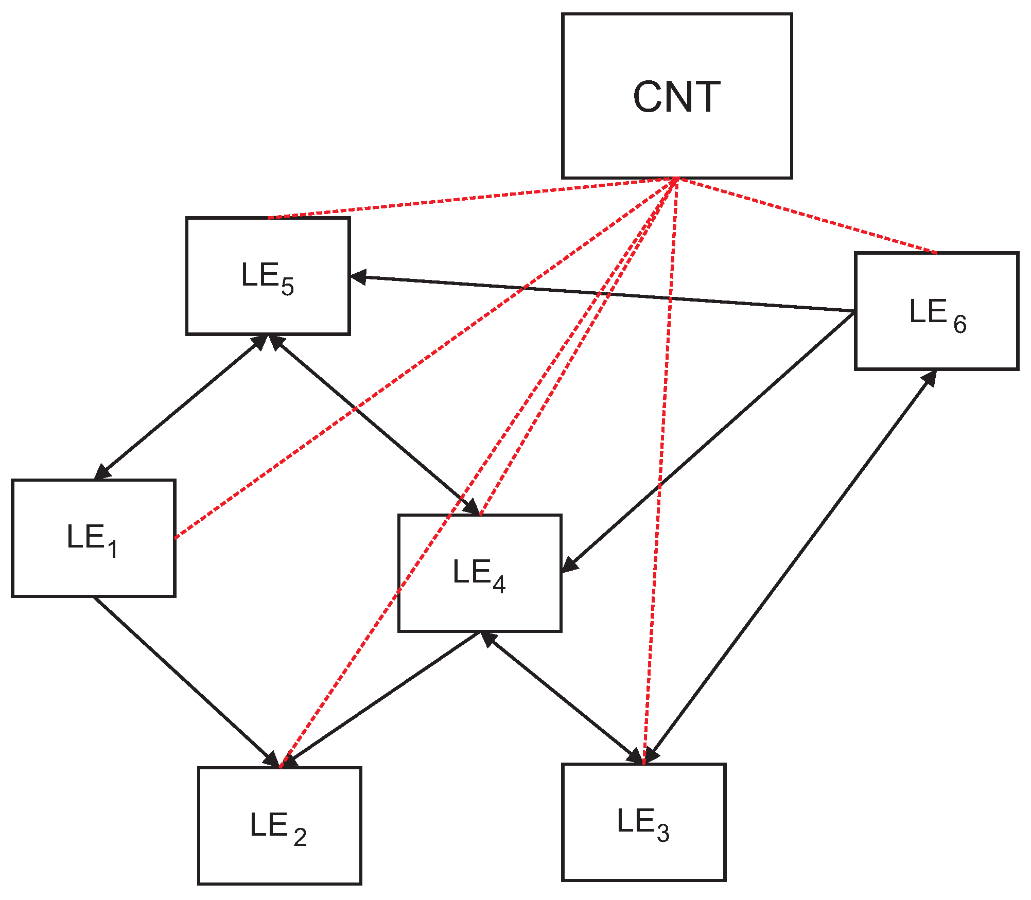
2. Distributed Calculation of Iterated Possible-Failure Scenarios

Let us consider a distributed peer-to-peer system, where the LEs work asynchronously and send information to the CNT when a stable result (convergence) from their calculations is obtained, of course repeating the procedure when the situation changes (Figure 1).
Assume that the scenarios are calculated in a way similar to weather forecasts, that is they may be determined on different horizons and they are updated repetitively at times t c , c = 0 , 1 , 2 , 3 , with a given frequency, e.g., for every 15 min, half an hour, etc. The calculations of these scenarios are performed before every t c , that is at the end of the interval ( t c 1 , t c ) . Assume also that an LE delivers a service s. The set of all services considered by us will be denoted by S. At a given time t k s ( t c 1 , t c ) , while analyzing the risk of its malfunctioning, the s-th LE considers a future time interval T s , which is composed of a number of subintervals T p s , p = 1 , , P s , that is:
T s = T 1 s T 2 s T P s s
For each of these intervals, let us denote with L s ( p , t k s ) the likelihood of a failure of a service s estimated at time t k s < t c . The possible failure scenario (PFS) of the service s estimated at time t k s is defined as L s ( t k s ) = ( L s ( p , t k s ) ; p = 1 , , P s ) . We assume, of course, that every local entity, using its risk assessment method, which takes into account its current cyber-security situation and PFSs of the neighbouring LEs influencing its functioning, is able to determine its own PFS.
Intervals T p s can have different lengths related to the different reaction times of various services. For example, for P s = 4 , T 1 s may refer to a short nearest-future period in which the service s may be affected by current threats. The next, longer, intervals T 2 s , T 3 s (mid term) and T 4 s (long term) (Figure 2) may concern both the threats and reactions on them.
PFSs of essential services will deliver the most important information, and may be used, e.g., for analysis, graphical threat presentation, and, in cases when it is possible to determine numerical cost values for PFSs, for the optimization of different safety measures that may be applied during the incident.

3. LE Working Mode

Now, consider the risk assessment at the local unit level. Suppose that the s-th LE information system has multiple vulnerabilities v V s , exploited by a number of cyber threats m M s , where V s is the set of vulnerabilities, and M s is the set of cyber threats affecting the service s. The vulnerability v V s is exploited with an impact factor I v s on the likelihood of the failure/degradation of the service provided by LE. These impacts may be expressed with appropriate numbers attached, e.g., [25]: low (0, 0.1), medium (0.1, 0.5), and high (0.5, 1). For each threat m M s , it is possible to assign a likelihood L v m s that this threat may exploit vulnerability v V s , and to define the risk activation function as:
R m s ( p ) = 1 when   threat   m   is   expected to   be   present   within   T p s 0 otherwise
Moreover, except these local cyber threats, it may be that the external services influencing s-th LE can also be temporarily disrupted or substantially degraded. Let us denote the set of those entities by U s and the impact of the failure of the service u on the service s by J u s . It is assumed that all compromised services can work in the safe mode, which implies that their likelihood of failure is restricted to L ¯ u , u U s .
Summing up, the likelihood that the service s will fail in the subinterval T p s , issued at time t k + 1 s > t k s , such that t k + 1 s < t c , can be be calculated as follows:
L s ( p , t k + 1 s ) = v V s I v s m M s L v m s R m s ( p )
+ u U s J u s min L ¯ u , L u r u s ( p ) , τ u s ( t k s )
where p = 1 , , P s . The argument r u s ( p ) , indicates the subinterval of T u relevant for the estimation of L s ( p , t k + 1 s ) , the argument τ u s ( t k s ) < t k s is the time from which the image of PFS of the service u possessed by the s t h LE at time t k s comes [7].
Iterations of the algorithm (3) are performed until convergence, which can be detected, e.g., by one of the protocol-free algorithms [26] or by the classical graph algorithm based on the acknowledgment messages [7]. During the iterations, it may happen that the information available at a LE level changes due to, for example, new incidents. This will affect the iterative process and the results until achieving a new stable forecast.

4. Convergence of the Algorithm

Let us analyze the conditions under which the algorithm (3) converges.
In fact, the first sum in (3) is constant in subsequent iterations, hence we may write this algorithm in the following way:
x : = F ( x )
where x R n is the vector of all variables L s ( p , t ) , p = 1 , , P s , s S for some t and for i = 1 , , n
F i ( x ) = b i + j i a i j min ( x ¯ j , x j )
Hence, in general, the algorithm (3) has the following form:
x i : = F i ( x ) =
b i + j i a i j min ( x ¯ j , x j ) , i = 1 , , n
The F ( x ) mapping is nonsmooth, so we cannot use the convergence formula on the nonlinear mappings from reference [7], based on the properties of the Jacobian matrix. Instead, we derive a sufficient convergence condition using a general theory of convergence for asynchronous iterative algorithms [7,8,9].
The basic theory says that a sufficient condition for the (4) algorithm to converge when implemented totally asynchronously is that the mapping F : R n R n is contractive in the maximum norm [7], i.e.,:
F ( x ) F ( y ) < x y x , y R n , x y
Theorem 1.
We consider a mapping F : R n R n with the coordinate functions defined as:
F i ( x ) = b i + j i a i j min ( x ¯ j , x j ) , i = 1 , , n
where the coefficients a i j are non-negative and such that:
j i a i j < 1 , i = 1 , , n
The mapping F is a contraction in the maximum norm.
Proof. 
Consider two arbitrary vectors x , y R n and define as i * = i * ( x , y ) an index of the coordinate determining the value of the maximum norm of x y , that is:
x y = max i = 1 , , n | x i y i | = | x i * y i * |
Due to the definition (8) of functions F i and the assumption that all coefficients a i j are non-negative, we will get for the mapping F:
F ( x ) F ( y )
= max i = 1 , , n | j i a i j min ( x ¯ j , x j ) min ( x ¯ j , y j ) |
max i = 1 , , n j i a i j | min ( x ¯ j , x j ) min ( x ¯ j , y j ) |
Let us analyze deeper the term:
| min ( x ¯ j , x j ) min ( x ¯ j , y j ) |
There are four combinations to analyze:
  • x j < x ¯ j y j < x ¯ j
    We have here:
    | min ( x ¯ j , x j ) min ( x ¯ j , y j ) | = | x j y j |
  • x j x ¯ j y j < x ¯ j
    We have here:
    | min ( x ¯ j , x j ) min ( x ¯ j , y j ) | = | x ¯ j y j |
    = x ¯ j y j x j y j | x j y j |
  • x j < x ¯ j y j x ¯ j
    We have here:
    | min ( x ¯ j , x j ) min ( x ¯ j , y j ) | = | x j x ¯ j |
    = x ¯ j x j y j x j | y j x j | = | x j y j |
  • x j x ¯ j y j x ¯ j
    We have here:
    | min ( x ¯ j , x j ) min ( x ¯ j , y j ) | = | x ¯ j x ¯ j | = 0
    | x j y j |
Thus, for all these cases there will be:
| min ( x ¯ j , x j ) min ( x ¯ j , y j ) | | x j y j |
Taking this, (10), and the assumption (9) into account in the assessment (11), it means that:
F ( x ) F ( y ) max i = 1 , , n j i a i j | x j y j |
max i = 1 , , n j i a i j | x i * y i * |
= | x i * y i * | max i = 1 , , n j i a i j < | x i * y i * | = x y
This means that F is a contractive mapping in the maximum norm. □

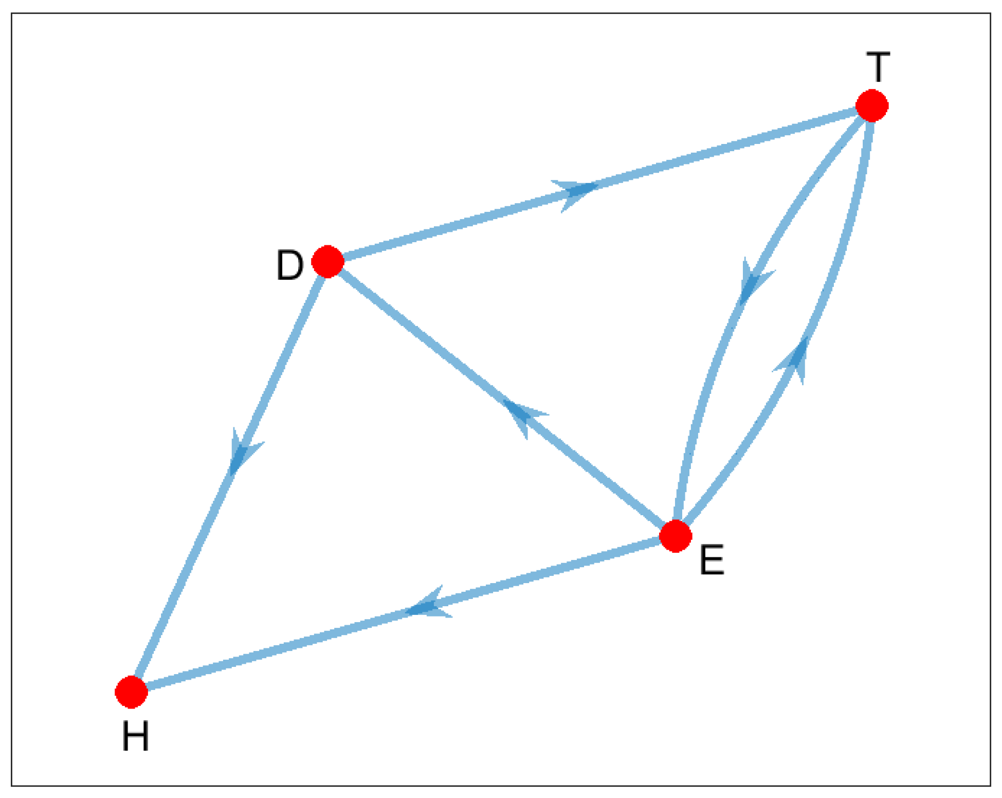
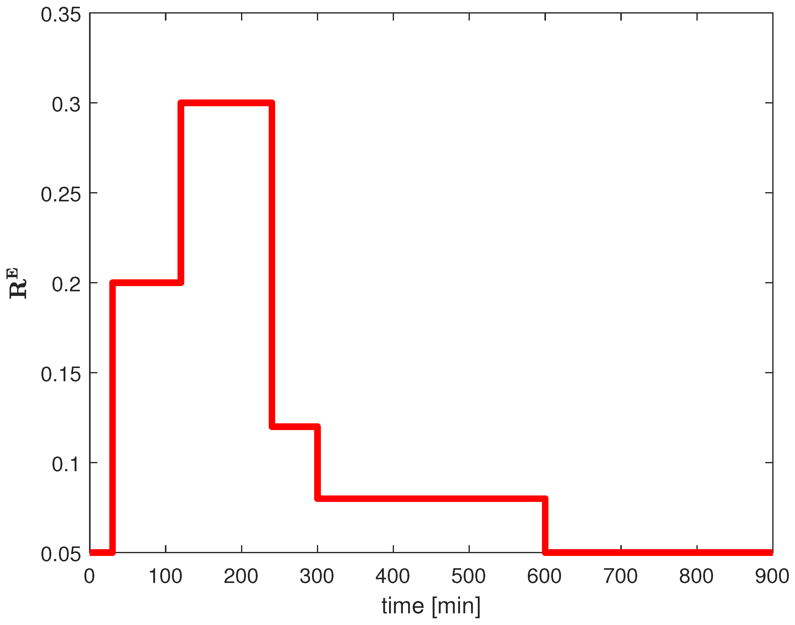
5. An Illustrative Example

To illustrate the ideas which were introduced above, let us consider an example of a system consisting of four service providers:
  • Power company responsible for both a local power plant and the distribution grid (E);
  • Railway transport company (T);
  • Hospital (H);
  • Data center (D).
All the services depend on electricity provided by the power company. In the case of a break in the energy supply, the hospital for few hours may use its own electricity generator and the data center has a UPS system, which holds its work for several dozen minutes. Except energy, some of the hospital and transport services depend also on access to the data center. The facility generating the electricity of the power plant is assumed to be coal fired and depends on the railway transport.
The graph of services and connections between them is presented in Figure 3.
Each local entity has its own information system that may be vulnerable and subject to various cyber threats, leading to the deterioration—in the extreme case to the safe mode level—of the service provided by this entity to its clients and to other entities. For example, the corruption of the control system of the power plant or the energy distribution network will lead to power outages in towns and in the countryside in the area served by the power company, including the hospital, the transport company, and the data center.
In all cases of the entities considered in the example, it is assumed that the Formula (3) is used to compute the possible service failure scenarios. The first term in (3), related to locally assessed threats, is aggregated to a given number:
R s ( p ) = v V s I v s m M s L v m s R m s ( p )
Let us assume that one night at 4 a.m. cyber criminals started a DDOS attack on the IT system controlling the power plant. The abnormally growing traffic was noticed by the operator of the computer network of the company. His predicted scenario of the attack is presented in Figure 4. Namely, he suspects that such a situation may last longer, and if so, the risk factor will rise after the next half an hour from the current normal R E ( 1 ) = 0.05 to a pre-alarm level R E ( 2 ) = 0.2 until 6 a.m., and then to the alarm level R E ( 3 ) = 0.3 until the end of the night shift at 8 a.m. At 8 a.m. the full IT staff will start their work and they will be gradually taking full control over the system and the local risk factors will decrease to R E ( 4 ) = 0.12 , R E ( 5 ) = 0.08 , R E ( 6 ) = 0.05 .
Now, starting from the power company (E), we assume the following timing and formulas defining the relevant scenarios:
L E ( p ) , p = 1 , 2 , , 6 ;
T E = [ 0 ,   30 ) [ 30 ,   120 ) [ 120 ,   240 ) [ 240 ,   300 )
[ 300 ,   600 ) [ 600 ,   900 ] min
L E ( p , t k + 1 E ) = R E ( p ) + 0.3 · min 0.5 , L T ( p 1 , τ T E ( t k E ) )
= 0.05 , p = 1 0.2 , p = 2 0.3 , p = 3 0.12 , p = 4 0.08 , p = 5 0.05 , p = 6 + 0.3 · min 0.5 , L T ( p 1 , τ T E ( t k E ) )
The expressions for likelihoods and possible failure scenarios for the transport company (T) will be as follows:
L T ( p ) , p = 1 , 2 , , 6 ;
T T = [ 0 ,   45 ) [ 45 ,   135 ) [ 135 ,   270 ) [ 270 ,   390 )
[ 390 ,   690 ) [ 690 ,   900 ] min
L T ( p , t k + 1 T ) = 0.06 + 0.7 · min ( 0.4 , L E ( p , τ E T ( t k T ) ) )
+ 0.25 · min ( 0.5 , L D ( p 1 , τ D T ( t k T ) ) )
The likelihoods and scenarios for the data center (D) are defined as:
L D ( p ) , p = 1 , 2 , , 6 ;
T D = [ 0 , 60 ) [ 60 ,   150 ) [ 150 ,   330 ) [ 330 ,   490 )
[ 490 ,   720 ) [ 720 ,   900 ] min
L D ( p , t k + 1 D ) = 0.08 + 0.2 · min ( 0.4 , L E ( p 1 , τ E D ( t k D ) ) ) ,
And, finally, for the hospital (H), the likelihoods and scenarios are specified as:
L H ( p ) , p = 1 , 2 , , 6 ;
T H = [ 0 ,   90 ) [ 90 ,   180 ) [ 180 ,   360 ) [ 360 ,   540 )
[ 540 ,   750 ) [ 750 ,   900 ] min
L H ( p , t k + 1 H ) = 0.07 + 0.2 · min ( 0.4 , L E ( p 1 , τ E H ( t k H ) ) )
+ 0.15 · min ( 0.5 , L D ( p 1 , τ D H ( t k H ) ) ) .
Despite the overall time horizon being 15 h for all local units, the duration of time subintervals varies between the different entities.
The results of the computations are presented in Figure 5. The simulation shows that the rise of the risk of failure in the delivery of electricity results at about 4:30 a.m. in an almost immediate (more precisely, after 15 min) jump growth of the likelihood of failure of the railway transport system, and a little later we can see a similar, but smaller, effect for the data center (after an hour from the beginning of the incident, that is time “0”), and for the hospital (after 1.5 h from time “0”). Fortunately, when the day shift IT staff arrive to work at 8 a.m. (4 h from the beginning of the attack) this risk is attenuated, and this implies the decrease of the likelihood of failure, first of the power plant and then, in the same order as for the degradation, of the other services.

6. Conclusions

In the paper a distributed, predictive, online scheme for national-level risk assessments was proposed. In this scheme, local entities, delivering different important services, repetitively prepare their own assessments, taking into account the temporal dependencies of their services on local cyber threats and services provided by other entities. The iterative, asynchronously convergent algorithm, which calculates the local scenarios, takes into account interdependencies between different services as a linear combination of local and external components. Due to the restriction on the influence function of the external components, the resulting mapping is nonlinear and nonsmooth. It was proved that when the sum of the weights of the external units is less than one, this mapping is a contraction in the maximum norm and the algorithm is convergent. It was confirmed in a numerical case study concerning a system consisting of four entities. Particular attention was paid to the scenario of the external attack on one of the units. This scenario, that is its risk assessment, may depend on local decisions, e.g., the number of staff working in different hours. If this dependence can be described formally, the presented model with slight modifications can be used also for optimization and planning purposes. This will be the subject of future works. The deployment of these distributed, asynchronous mechanisms will speed up the development of decisions to protect the network from attacks and reduce their negative impacts on society and the economy.

Funding

This research received no external funding.

Conflicts of Interest

The author declares no conflict of interest.

Abbreviations

The following symbols were used in the manuscript:
CNTOperations Center
LElocal entity delivering a service
L E i i-th local entity in the system
PFSpossible failure scenario
t c time of calculation of the c-th set of possible failure scenarios
for the whole system
t k s 
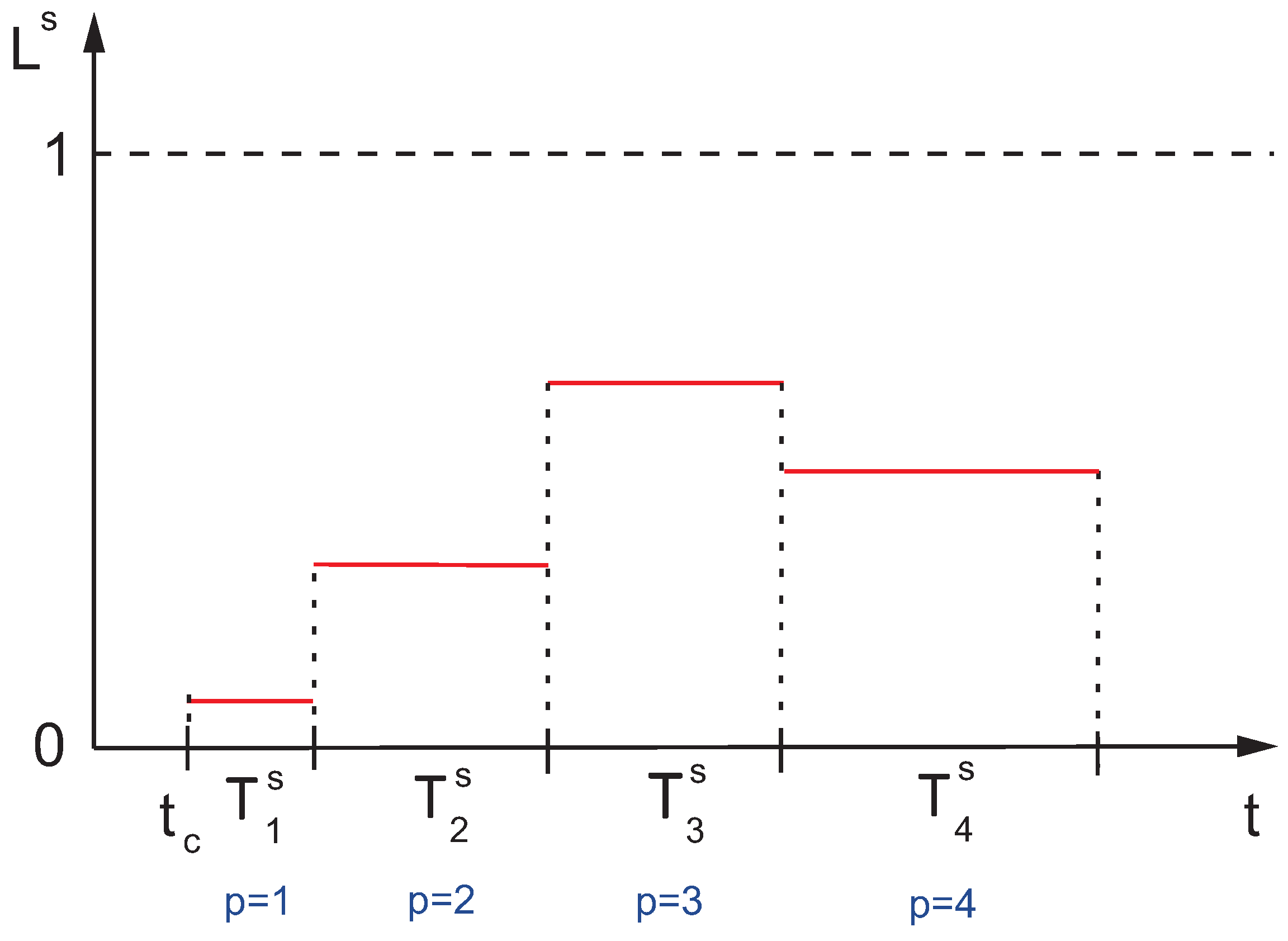
time of the k-th iteration of calculation of the PFS of the service s
P s number of subintervals of the PFSs issued by the service (node) s
L s ( t k s ) the possible failure scenario (PFS) of the service s estimated at time t k s
L s ( p , t k s ) p-th element of the scenario (sequence) L s ( t k s )
T s time interval of the PFSs issued by the s-th LE
T p s p-th subinterval of T s
V s set of vulnerabilities of the s -th LE information system
M s set of cyber threats affecting the service s
L v m s likelihood that the m-th threat may exploit vulnerability v V s of the service s
R m s ( p ) risk activation function of a threat m M s for the service s
in the p-th subinterval of its PFS
R s ( p ) aggregated risk activation function for the service s
in the p-th subinterval of its PFS
I v s impact factor of the vulnerability v V s on the failure/degradation
of the service provided by the s-th LE
U s set of the external services influencing s-th LE
J u s impact factor of the failure of the service u on the service s
r u s ( p ) the subinterval of T u relevant for the estimation of L s ( p , t k + 1 s )
τ u s ( t k s ) time from which the image of PFS of the service u possessed by the s-th LE
at time t k s stems
L ¯ u the maximal likelihood of failure of a service u U s

References

  1. Yadav, R. Cyber Security Threats During COVID-19 Pandemic. Int. Trans. J. Eng. Manag. Appl. Sci. Technol. 2021, 12, 12A3Q. [Google Scholar]
  2. Shah, A.; Ganesan, R.; Jajodia, S.; Samarati, P.; Cam, H. Adaptive Alert Management for Balancing Optimal Performance among Distributed CSOCs using Reinforcement Learning. IEEE Trans. Parallel Distr. Syst. 2020, 31, 16–33. [Google Scholar] [CrossRef]
  3. Baz, M.; Alhakami, H.; Agrawal, A.; Baz, A.; Khan, R.A. Impact of COVID-19 Pandemic: A Cybersecurity Perspective. Intell. Autom. Soft Comput. 2021, 27, 641–652. [Google Scholar] [CrossRef]
  4. European Commission, Joint Research Centre. Recommendations for National Risk Assessment for Disaster Risk Management in EU; Publications Office of the European Union: Luxembourg, 2021. [Google Scholar]
  5. Malinowski, K.; Karbowski, A. Real-Time Hierarchical Predictive Risk Assessment at National Level; Mutually Agreed Predicted Service Disruption Profiles. Int. J. Appl. Math. Comput. Sci. 2020, 30, 597–609. [Google Scholar]
  6. Karbowski, A.; Malinowski, K. Two-Level System of on-Line Risk Assessment in the National Cyberspace. IEEE Access 2020, 8, 181404–181410. [Google Scholar] [CrossRef]
  7. Bertsekas, D.P.; Tsitsiklis, J.N. Parallel and Distributed Computation: Numerical Methods; Athena Scientific: Belmont, MA, USA, 2015. [Google Scholar]
  8. Karbowski, A. Distributed, Asynchronous Algorithms for Data Networks Control—A State of the Art Review. In Artificial Intelligence and Computer Science; Shannon, S., Ed.; Nova Science Publishers, Inc.: Commack, NY, USA, 2005; pp. 59–82. [Google Scholar]
  9. Karbowski, A. Comments on Optimization Flow Control, I: Basic Algorithm and Convergence. IEEE/ACM Trans. Netw. 2003, 11, 338–339. [Google Scholar] [CrossRef]
  10. Mirzaei, O.; de Fuentes, J.M.; González Manzano, L. Dynamic Risk Assessment in IT Environments: A Decision Guide. In Handbook of Research on Information and Cyber Security in the Fourth Industrial Revolution; Fields, Z., Ed.; IGI Global: Hershey, PA, USA, 2018; pp. 234–261. [Google Scholar]
  11. Pirbhulal, S.; Gkioulos, V.; Katsikas, S. A Systematic Literature Review on RAMS analysis for critical infrastructures protection. Int. J. Crit. Infrastruct. Prot. 2021, 33, 100427. [Google Scholar] [CrossRef]
  12. Brændelanda, G.; Refsdal, A.; Stølen, K. Modular analysis and modelling of risk scenarios with dependencies. J. Syst. Softw. 2010, 83, 1995–2013. [Google Scholar] [CrossRef]
  13. Theoharidou, M.; Kotzanikolaou, P.; Gritzalis, D. Risk assessment methodology for interdependent critical infrastructures. Int. J. Risk Assess. Manag. 2011, 15, 128–148. [Google Scholar] [CrossRef]
  14. Gonzalez-Granadillo, G.; Dubus, S.; Motzek, A.; Garcia-Alfaro, J.; Alvarez, E.; Merialdo, M.; Papillon, S.; Debar, H. Dynamic risk management response system to handle cyber threats. Future Gener. Comput. Syst. 2018, 83, 535–555. [Google Scholar] [CrossRef]
  15. Bhuiyan, T.H.; Medal, H.R.; Nandi, A.K.; Halappanavar, M. Risk-averse bi-level stochastic network interdiction model for cyber-security risk management. Int. J. Crit. Infrastruct. Prot. 2021, 32, 100408. [Google Scholar] [CrossRef]
  16. Naumov, S.; Kabanov, I. Dynamic framework for assessing cyber security risks in a changing environment. In Proceedings of the 22nd International Conference on Information and Software Technologies ICIST 2016, Druskininkai, Lithuania, 13–15 October 2016. [Google Scholar]
  17. Amin, M.T.; Khan, F.; Ahmed, S.; Imtiaz, S. A novel data-driven methodology for fault detection and dynamic risk assessment. Can. J. Chem. Eng. 2020, 98, 2397–2416. [Google Scholar] [CrossRef]
  18. Ye, N.; Zhang, Y.; Borror, C.M. Robustness of the Markov-Chain Model for Cyber-Attack Detection. IEEE Trans. Reliab. 2004, 53, 116–123. [Google Scholar] [CrossRef]
  19. Karbowski, A.; Malinowski, K.; Szwaczyk, S.; Jaskóła, P. Critical Infrastructure Risk Assessment Using Markov Chain Model. J. Telecommun. Inf. Technol. 2019, 2019, 15–20. [Google Scholar] [CrossRef]
  20. Hu, B.; Zhou, C.; Tian, Y.-C.; Hu, X.; Junping, X. Decentralized Consensus Decision-Making for Cybersecurity Protection in Multimicrogrid Systems. IEEE Trans. Syst. Man Cybern. Syst. 2021, 51, 2187–2198. [Google Scholar] [CrossRef]
  21. European Union Agency for Network and Information Security. National-level Risk Assessments an Analysis Report—Executive Summary Nov. 2013; ENISA: Heraklion, Greece, 2013.
  22. Kure, H.I.; Islam, S.; Razzaque, M.A. An Integrated Cyber Security Risk Management Approach for a Cyber-Physical System. Appl. Sci. 2018, 8, 898. [Google Scholar] [CrossRef] [Green Version]
  23. Riesco, R.; Villagrá, V.A. Leveraging cyber threat intelligence for a dynamic risk framework. Int. J. Inf. Secur. 2019, 18, 715–739. [Google Scholar] [CrossRef]
  24. Kavallieratos, G.; Spathoulas, G.; Katsikas, S. Cyber Risk Propagation and Optimal Selection of Cybersecurity Controls for Complex Cyberphysical Systems. Sensors 2021, 21, 1691. [Google Scholar] [CrossRef] [PubMed]
  25. National Institute of Standards and Technology, U.S. Department of Commerce. Guide for Conducting Risk Assessments, Information Security. NIST Special Publication 800—30 Revision 1; National Institute of Standards and Technology: Gaithersburg, MD, USA, 2012.
  26. Gbikpi-Benissan, G.; Magoulèsb, F. Protocol-free asynchronous iterations termination. Adv. Eng. Softw. 2020, 146, 102827. [Google Scholar] [CrossRef]
Figure 1. Distributed system of online risk assessment: L E 1 , , L E 6 —local entities delivering services; CNT—Operations Center. Arrows on links show dependencies between services and the information flow during calculations. The red (dotted) lines represent exchange of information between subsequent computations.
Electronics 11 00741 g001
Figure 2. Exemplary possible failure scenario; L s —level of likelihood of failure of the service s during time interval T s consisting of 4 subintervals: T 1 s , T 2 s , T 3 s , T 4 s .
Electronics 11 00741 g002
Figure 3. Graph of services and dependencies: Notation: E—power company; T—transport company; H—hospital; D—data center.
Electronics 11 00741 g003
Figure 4. Scenario of an attack on the power plant.
Electronics 11 00741 g004
Figure 5. Possible failure scenarios for the whole system after an attack on the power plant.
Electronics 11 00741 g005
Publisher’s Note: MDPI stays neutral with regard to jurisdictional claims in published maps and institutional affiliations.

