
An Intelligent Data Analysis System Combining ARIMA and LSTM for Persistent Organic Pollutants Concentration Prediction


Abstract
:1. Introduction
2. Related Work
3. Our Proposed Intelligent System
3.1. Baseline Models
3.1.1. ARIMA Model
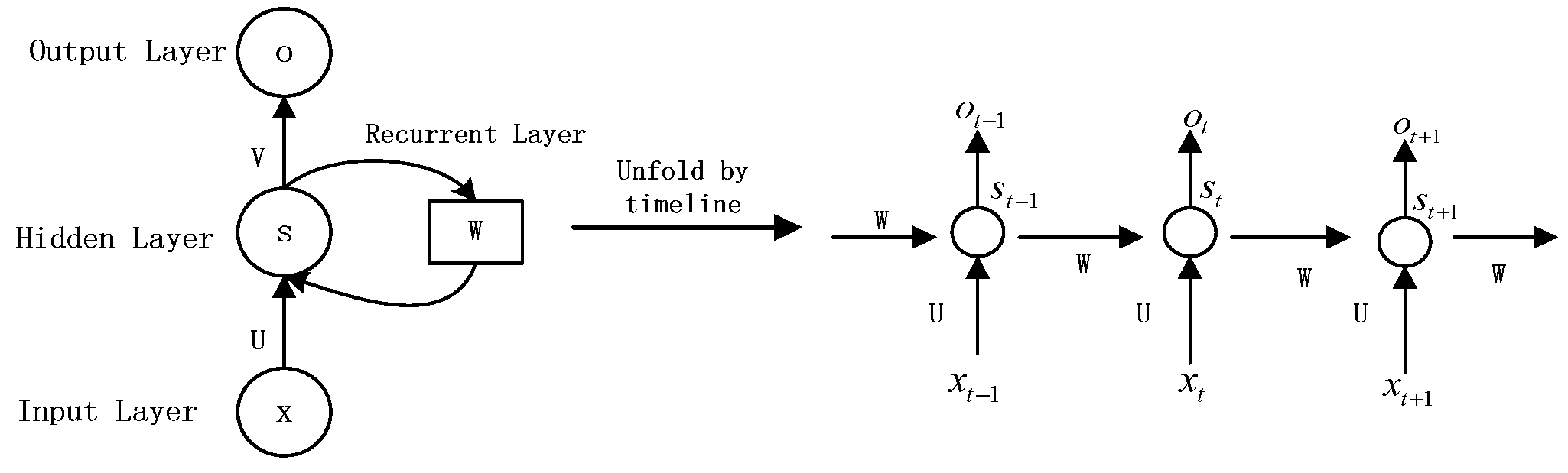
3.1.2. RNN Model
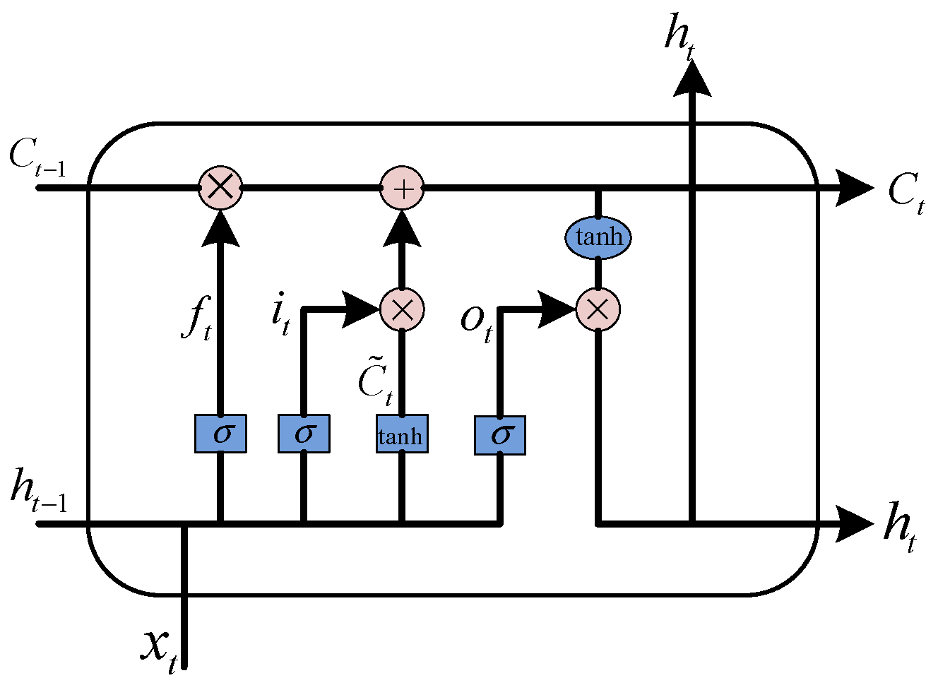
3.1.3. LSTM Model
3.2. Our Proposed Intelligent System Combining ARIMA and LSTM
| Algorithm 1. Description of algorithm of our system. |
| Input: x is concentration sequence |
| Output: predicted values |
| # Obtain linear predictions from ARIMA model |
| ADF(x) d = 0 while x is not stationary do x = diff(x) d = d + 1 end while |
| for p in range(1,pmax + 1) |
| for q in range(1,qmax + 1) |
| model = ARIMA(x,(p,d,q)) |
| BIC = bic(model) |
| end for |
| end for |
| p,q = Minindex(BIC) |
| model = ARIMA(x,(p,d,q)) |
| L, e = model.predict() # linear predictions and residuals |
| # Obtain residual predictions from the first LSTM |
| training_set = create_datasets(e,x,d) # d is external factors |
| op = get the optimal hyperparameter using grid search |
| model1 = Sequential() |
| model1.add(LSTM(op)) |
| model1.compile(loss = ’mse’, optimizer = ’adam’) |
| model1.fit(training_set) |
| N = model1.predict() # residual predictions |
| # Obtain the predictions from the second LSTM |
| training_set1 = create_datasets(N, L) |
| op1 = get the optimal hyperparameter using grid search |
| model2 = Sequential() |
| model2.add(LSTM(op1)) |
| model2.compile(loss = ’mse’, optimizer = ’adam’) |
| model2.fit(training_set1) |
| model2.predict() # predictions |
4. Experiments and Performance Analysis
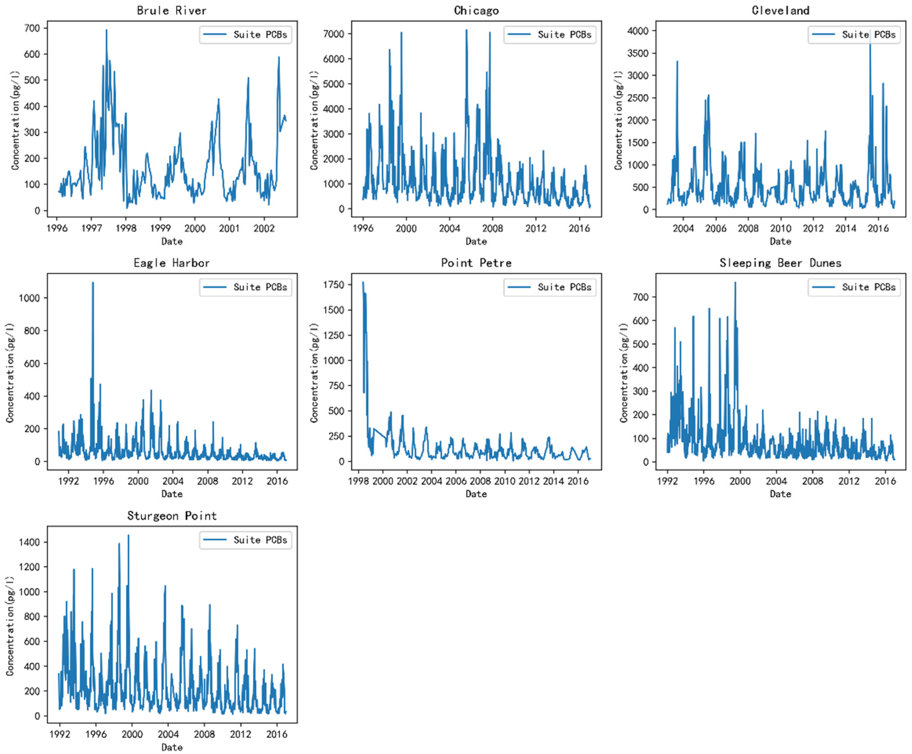
4.1. Datasets
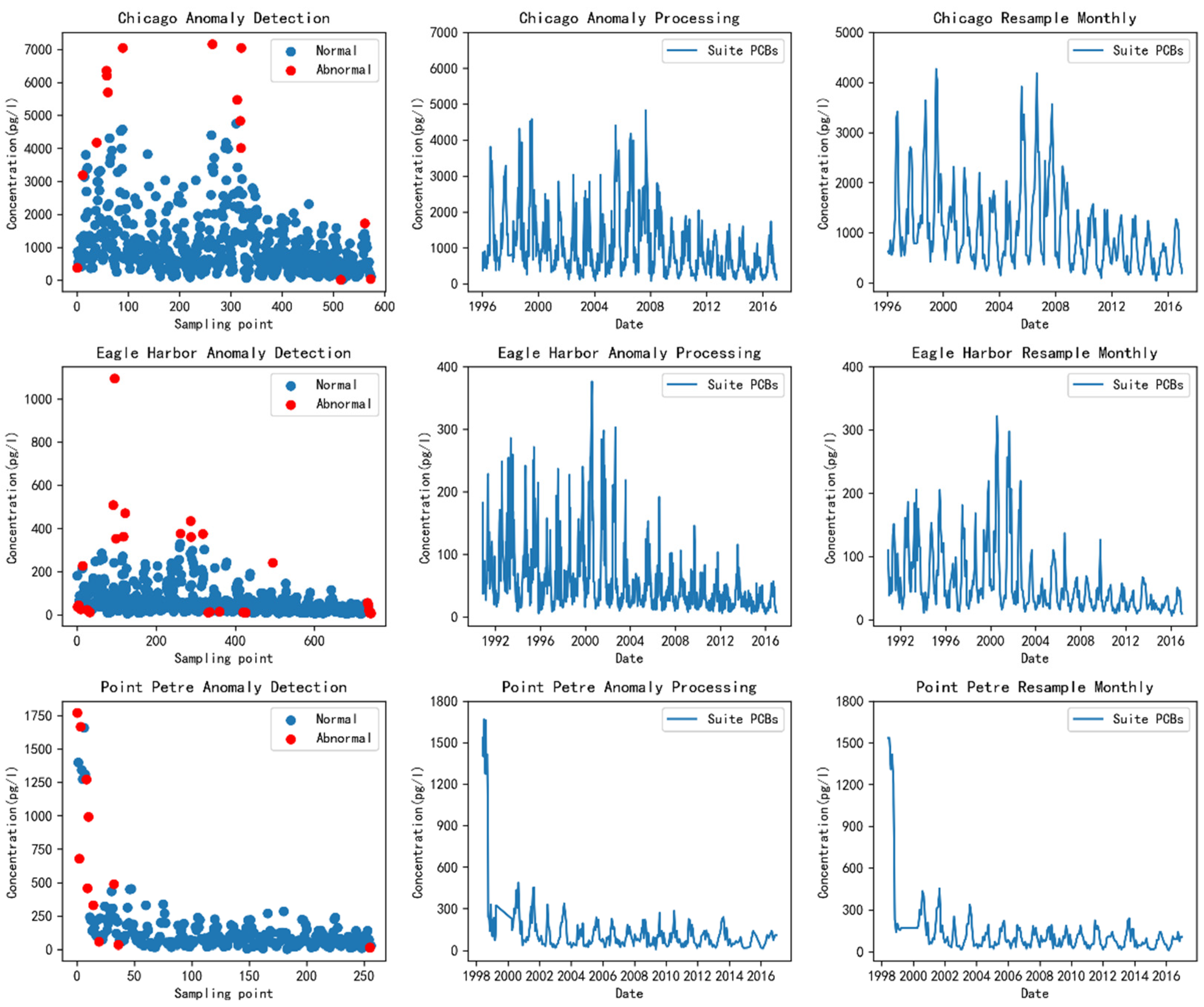
4.2. Data Preprocessing
4.3. Parameter Tuning
4.3.1. Parameter Setting for ARIMA
- Determine the value of d. Augmented Dickey Fuller (ADF) test [55] is applied to test the stability of concentration sequence. The essence of ADF test is to judge whether the sequence has a unit root. If sequence is stationary, there is no unit root. If the p-value > 0.05, we cannot reject the null hypothesis (H0) and the sequence has a unit root. Then the subsequent difference operation must be performed. The ADF test was applied to Chicago, Eagle Harbor and Point Petre, respectively, and the results are shown in Table 2. If the ADF statistic value is less than the corresponding Critical Value, then there are, correspondingly, 99%, 95% and 90% probability of rejecting the null hypothesis. However, this paper uses the p-value to determine the value of d. The p-value of Chicago is 0.646, which is greater than 0.05, so a difference operation is required. Similarly, the p-value of Eagle Harbor is 0.363, which is also larger than 0.05, and a difference operation is also required. However, the p-value of Point Petre is 0.001, which is smaller than 0.05, and this series is stationary without difference operation.
- Determine the parameter order of p and q. The values of p and q are preliminarily determined according to their respective ACF and PACF graphs [55], and then BIC method [56] is used to choose the best parameter order, obtain the minimum value of BIC, and then the corresponding values of p, q are determined.
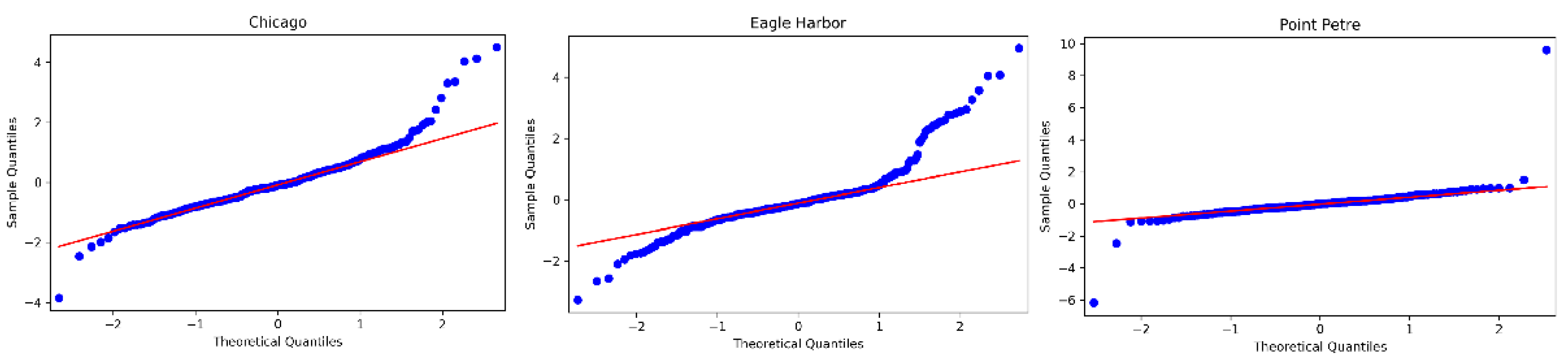
- Model evaluation. The test of model is mainly carried out from the following two aspects: Firstly, using the QQ chart [55] to test whether the residual is normally distributed. It can be seen from Figure 6 that the residuals of ARIMA model on the three datasets conform to the normal distribution. Secondly, the D–W (Durbin–Watson) [57] method is used to evaluate the auto-correlation of residuals. The corresponding D–W values are 2.0078, 2.0012, and 1.9988, respectively, which are all close to 2. Hence, there is no auto-correlation of residuals. Finally, the model for Chicago is ARIMA (8,1,3), Eagle Harbor is ARIMA (5,1,3), Point Petre is ARIMA (4,0,2).
4.3.2. Parameter Setting for RNN and LSTM
4.3.3. Parameter Setting for Our System
4.4. Performance Analysis
4.4.1. Evaluation Metrics
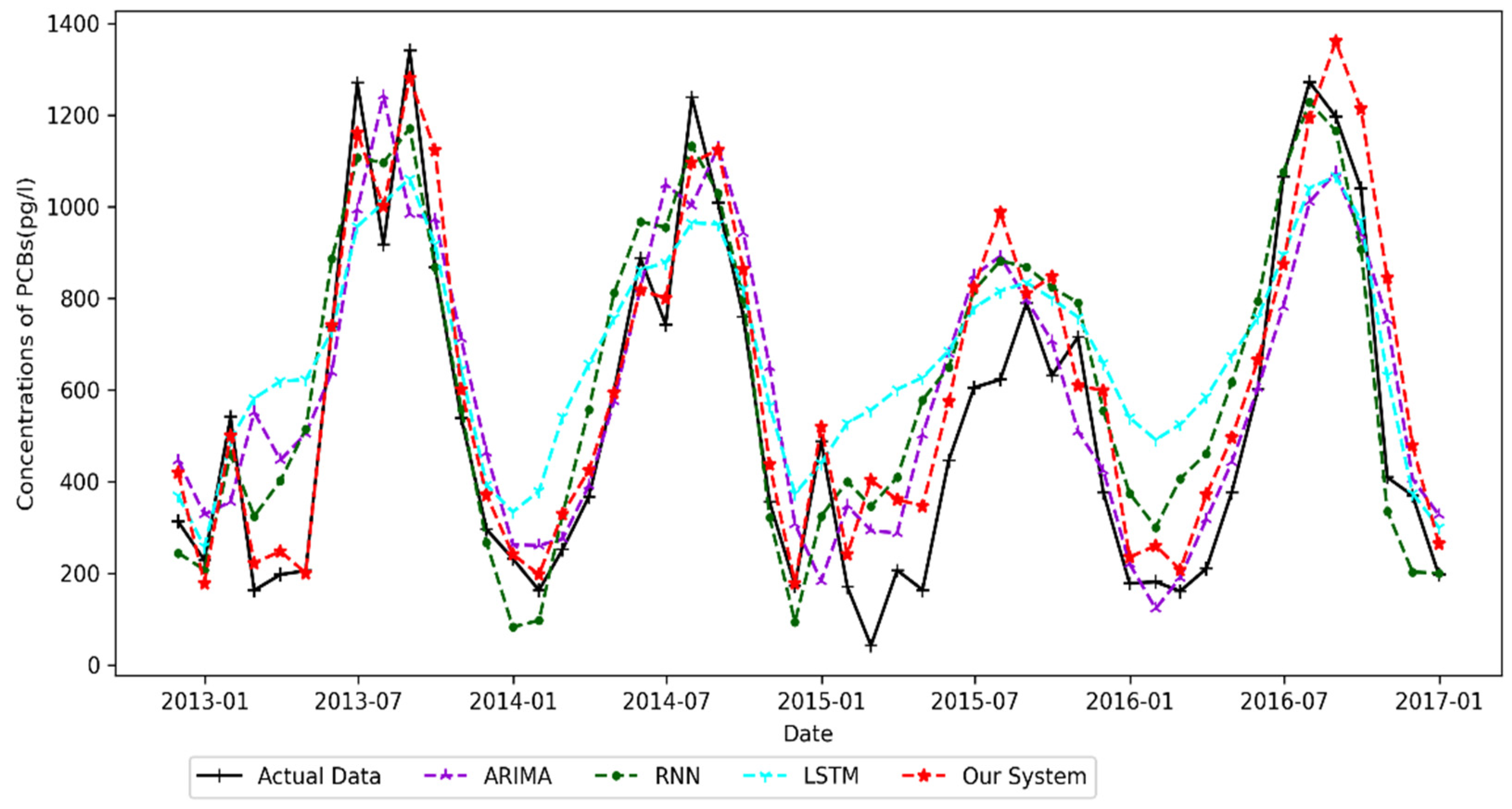
4.4.2. Chicago Result
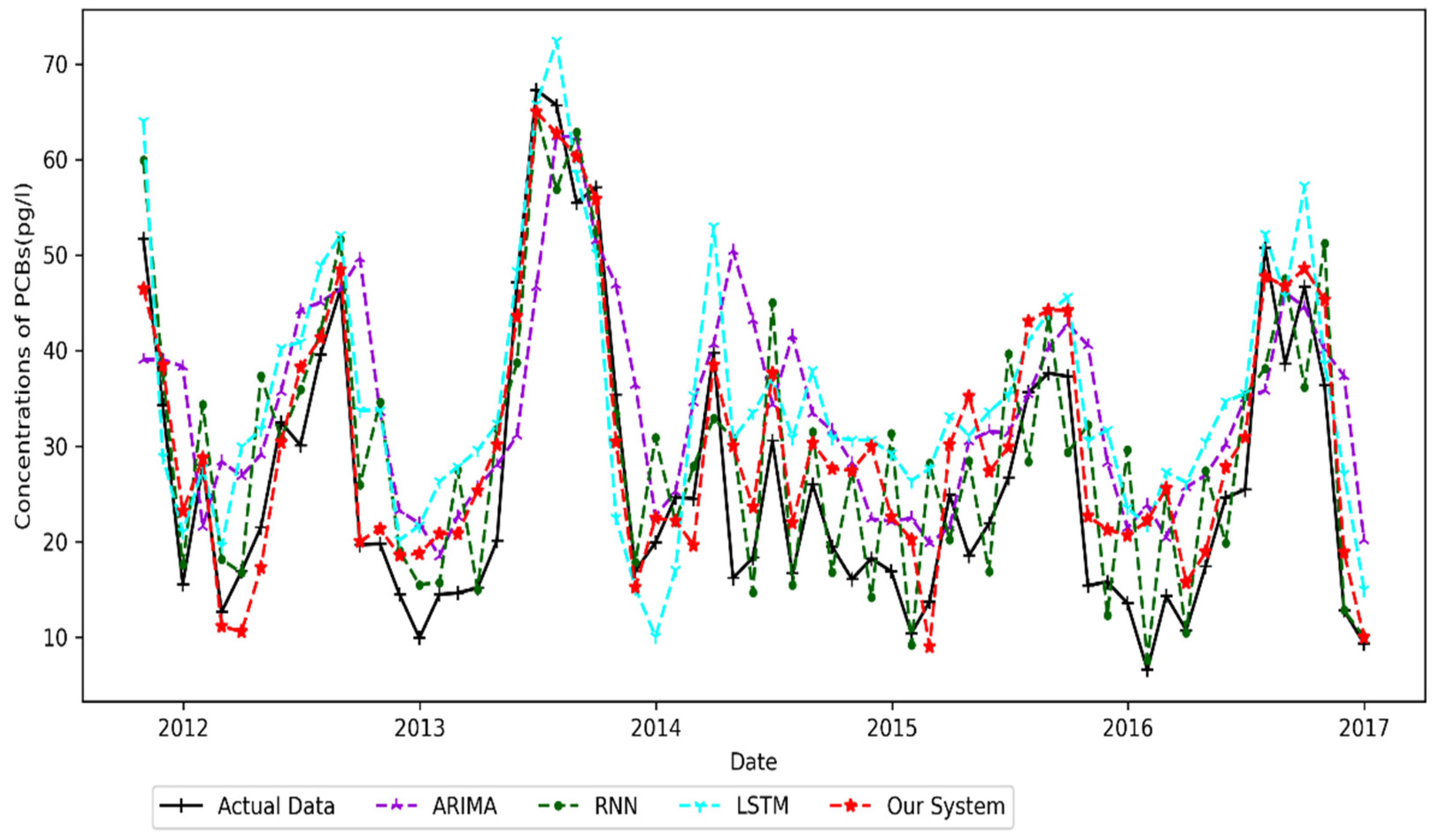
4.4.3. Eagle Harbor Result
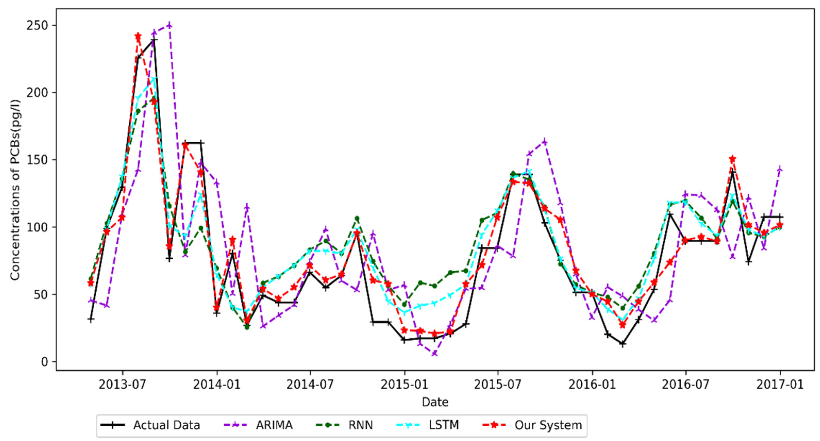
4.4.4. Point Petre Result
4.5. Future Prediction
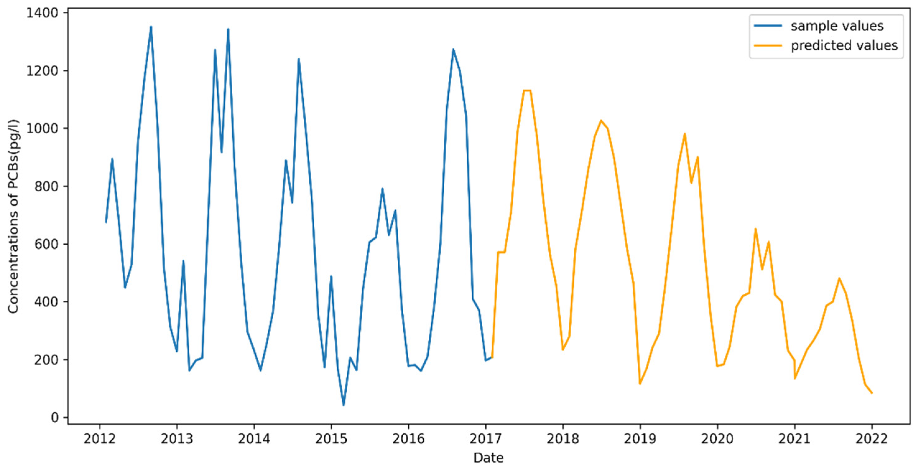
4.5.1. Chicago Prediction Result
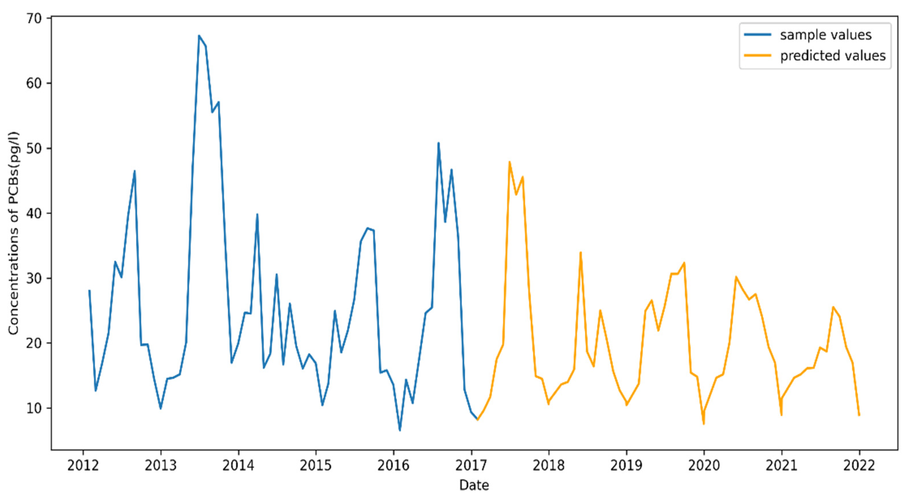
4.5.2. Eagle Harbor Prediction Result
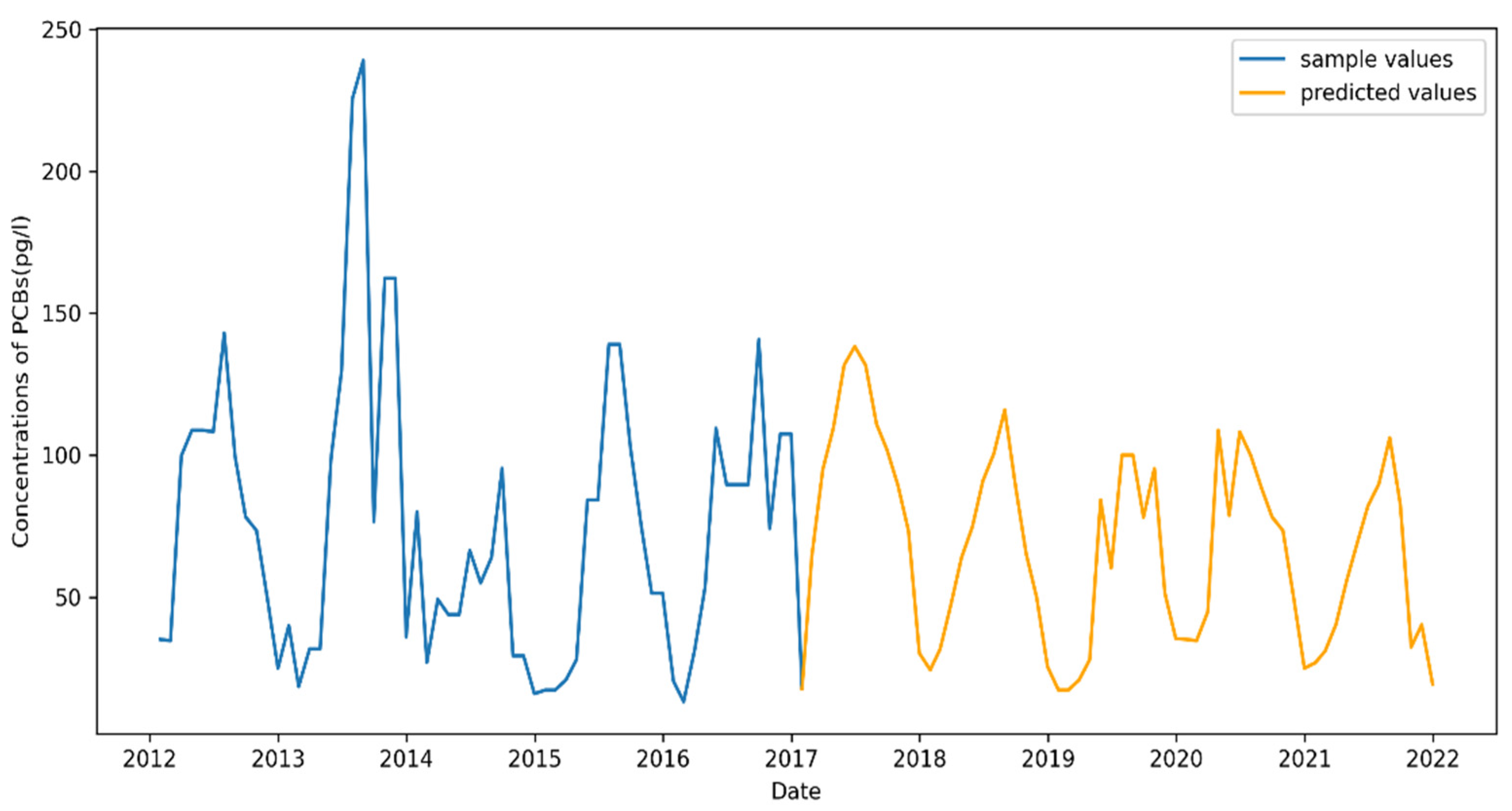
4.5.3. Point Petre Prediction Result
5. Conclusions and Future Work
Author Contributions
Funding
Data Availability Statement
Acknowledgments
Conflicts of Interest
References
- Magulova, K.; Priceputu, A. Global monitoring plan for persistent organic pollutants (POPs) under the Stockholm Convention: Triggering, streamlining and catalyzing global POPs monitoring. Environ. Pollut. 2016, 217, 82–84. [Google Scholar] [CrossRef] [PubMed]
- Zheng, M.; Tan, L.; Gao, L.; Ma, L.; Dong, S.; Yao, Y. Global Monitoring Plan of POPs Under the Stockholm Convention for Effectivenes Evaluation. Environ. Monit. China 2019, 35, 6–12. [Google Scholar]
- Ping, S.; Basu, I.; Blanchard, P.; Backus, S.M.; Hites, R.A. Temporal and Spatial Trends of Atmospheric Toxic Substances near the Great Lakes IADN Results Through 2003; Environment Canada and the United States Environmental Protection Agency: Chicago, IL, USA, 2002.
- Xia, F.; Hao, R.; Li, J.; Xiong, N.; Yang, L.T.; Zhang, Y. Adaptive GTS allocation in IEEE 802.15.4 for real-time wireless sensor networks. J. Syst. Archit. 2013, 59, 1231–1242. [Google Scholar] [CrossRef]
- Akyildiz, I.F.; Su, W.; Sankarasubramaniam, Y.; Cayirci, E. A Survey on Sensor Networks. IEEE Commun. Mag. 2002, 40, 102–114. [Google Scholar] [CrossRef] [Green Version]
- Gao, K.; Han, F.; Dong, P.; Xiong, N.; Du, R. Connected Vehicle as a Mobile Sensor for Real Time Queue Length at Signalized Intersections. Sensors 2019, 19, 2059. [Google Scholar] [CrossRef] [PubMed] [Green Version]
- Huang, S.; Liu, A.; Wang, T.; Xiong, N.N. BD-VTE: A Novel Baseline Data based Verifiable Trust Evaluation Scheme for Smart Network Systems. IEEE Trans. Netw. Sci. Eng. 2020, 8, 2087–2105. [Google Scholar] [CrossRef]
- Baothman, F.A. An Intelligent Big Data Management System Using Haar Algorithm-Based Nao Agent Multisensory Communication. Wirel. Commun. Mob. Comput. 2021, 2021, 9977751. [Google Scholar] [CrossRef]
- Yao, Y.; Xiong, N.; Park, J.H.; Ma, L.; Liu, J. Privacy-preserving max/min query in two-tiered wireless sensor networks. Comput. Math. Appl. 2013, 65, 1318–1325. [Google Scholar] [CrossRef]
- Wu, M.; Tan, L.; Xiong, N. A Structure Fidelity Approach for Big Data Collection in Wireless Sensor Networks. Sensors 2014, 15, 248. [Google Scholar] [CrossRef] [Green Version]
- Berthold, M.R.; Borgelt, C.; Höppner, F.; Klawonn, F. Intelligent Data Analysis; Springer: Berlin, Germany, 1999. [Google Scholar]
- Box, G.; Jenkins, G. Time Series Analysis Forecasting and Control. J. Time Ser. Anal. 1970, 3, 131–133. [Google Scholar]
- Jiang, Y.; Tong, G.; Yin, H.; Xiong, N. A Pedestrian Detection Method Based on Genetic Algorithm for Optimize XGBoost Training Parameters. IEEE Access 2019, 7, 118310–118321. [Google Scholar] [CrossRef]
- Paula, A.J.; Ferreira, O.P.; Filho, A.G.S.; Filho, F.N.; Andrade, C.E.; Faria, A.F. Machine Learning and Natural Language Processing Enable a Data-Oriented Experimental Design Approach for Producing Biochar and Hydrochar from Biomass. Chem. Mater. 2022, 34, 979–990. [Google Scholar] [CrossRef]
- He, R.; Xiong, N.; Yang, L.T.; Park, J.H. Using Multi-Modal Semantic Association Rules to fuse keywords and visual features automatically for Web image retrieval. Inf. Fusion 2011, 12, 223–230. [Google Scholar] [CrossRef]
- Li, H.; Liu, J.; Wu, K.; Yang, Z.; Liu, R.W.; Xiong, N. Spatio-Temporal Vessel Trajectory Clustering Based on Data Mapping and Density. IEEE Access 2018, 6, 58939–58954. [Google Scholar] [CrossRef]
- Wang, Y.; Li, Y.; Sui, J.; Gao, Y. Data Factory: An Efficient Data Analysis Solution in the Era of Big Data. In Proceedings of the 2020 5th IEEE International Conference on Big Data Analytics (ICBDA), Xiamen, China, 8–11 May 2020. [Google Scholar]
- Wang, Z.; Li, T.; Xiong, N.; Pan, Y. A novel dynamic network data replication scheme based on historical access record and proactive deletion. J. Supercomput. 2012, 62, 227–250. [Google Scholar] [CrossRef]
- Yang, P.; Xiong, N.N.; Ren, J. Data Security and Privacy Protection for Cloud Storage: A Survey. IEEE Access 2020, 8, 131723–131740. [Google Scholar] [CrossRef]
- Dien, N.T.; Hirai, Y.; Koshiba, J.; Sakai, S.I. Factors affecting multiple persistent organic pollutant concentrations in the air above Japan: A panel data analysis. Chemosphere 2021, 277, 130356. [Google Scholar] [CrossRef]
- Guo, W.; Xiong, N.; Vasilakos, A.V.; Chen, G.; Cheng, H. Multi-Source Temporal Data Aggregation in Wireless Sensor Networks. Wirel. Pers. Commun. 2011, 56, 359–370. [Google Scholar] [CrossRef]
- Yin, J.; Lo, W.; Deng, S.; Li, Y.; Wu, Z.; Xiong, N. Colbar: A collaborative location-based regularization framework for QoS prediction. Inf. Sci. Int. J. 2014, 265, 68–84. [Google Scholar] [CrossRef]
- Simcik, M.F.; Basu, I.; Sweet, C.W.; Hites, R.A. Temperature Dependence and Temporal Trends of Polychlorinated Biphenyl Congeners in the Great Lakes Atmosphere. Environ. Sci. Technol. 1999, 33, 1991–1995. [Google Scholar] [CrossRef]
- Sun, P.; Basu, I.; Hites, R.A. Temporal trends of polychlorinated biphenyls in precipitation and air at Chicago. Environ. Sci. Technol. 2006, 40, 1178. [Google Scholar] [CrossRef] [PubMed]
- Hites, R.A. Statistical Approach for Assessing the Stockholm Convention’s Effectiveness: Great Lakes Atmospheric Data. Environ. Sci. Technol. 2019, 53, 8585–8590. [Google Scholar] [CrossRef] [PubMed]
- Venier, M.; Salamova, A.; Hites, R.A. Temporal trends of persistent organic pollutant concentrations in precipitation around the Great Lakes. Environ. Pollut. 2016, 217, 143–148. [Google Scholar] [CrossRef] [PubMed]
- Zhao, Y. Statistical Analysis of Climate Change Signals in Typical Persistent Organic Pollutants in the Arctic and Great Lakes Regions. Ph.D. Thesis, Lanzhou University, Lanzhou, China, 2017. [Google Scholar]
- Yuan, Q. Prediction of Air/Particulate Matter Partition Coefficient (K_p) for Some Persistent Organic Pollutants; Zhejiang Normal University: Jinhua, China, 1956. [Google Scholar]
- Jones, K.C. Persistent Organic Pollutants (POPs) and Related Chemicals in the Global Environment: Some Personal Reflections. Environ. Sci. Technol. 2021, 55, 9400–9412. [Google Scholar] [CrossRef]
- Girones, L.; Oliva, A.L.; Negrin, V.L.; Marcovecchio, J.E.; Arias, A.H. Persistent organic pollutants (POPs) in coastal wetlands: A review of their occurrences, toxic effects, and biogeochemical cycling. Mar. Pollut. Bull. 2021, 172, 112864. [Google Scholar] [CrossRef]
- Zhang, Q.; Zhou, C.; Tian, Y.C.; Xiong, N.; Qin, Y.; Hu, B. A Fuzzy Probability Bayesian Network Approach for Dynamic Cybersecurity Risk Assessment in Industrial Control Systems. IEEE Trans. Ind. Inform. 2018, 14, 2497–2506. [Google Scholar] [CrossRef] [Green Version]
- Zhu, T.; Tao, C. Prediction models with multiple machine learning algorithms for POPs: The calculation of PDMS-air partition coefficient from molecular descriptor. J. Hazard. Mater. 2021, 423, 127037. [Google Scholar] [CrossRef]
- Das, M.; Ghosh, S.K. A probabilistic approach for weather forecast using spatio-temporal inter-relationships among climate variables. In Proceedings of the 2014 9th International Conference on Industrial and Information Systems (ICIIS), Gwalior, India, 15–17 December 2014; IEEE: Manhattan, NY, USA, 2014. [Google Scholar]
- Mellit, A.; Pavan, A.M.; Benghanem, M. Least squares support vector machine for short-term prediction of meteorological time series. Theor. Appl. Climatol. 2013, 111, 297–307. [Google Scholar] [CrossRef]
- Wu, C.; Wang, C.; Fan, Q.; Wu, Q.; Xu, S.; Xiong, N.N. Design and Analysis of an Data-Driven Intelligent Model for Persistent Organic Pollutants in the Internet of Things Environments. IEEE Access 2021, 9, 13451–13463. [Google Scholar] [CrossRef]
- Alabdulrazzaq, H.; Alenezi, M.N.; Rawajfih, Y.; Alghannam, B.A.; Al-Hassan, A.A.; Al-Anzi, F.S. On the accuracy of ARIMA based prediction of COVID-19 spread. Results Phys. 2021, 27, 104509. [Google Scholar] [CrossRef]
- Zhao, Y.; Wang, L.; Luo, J.; Huang, T.; Ma, J. Deep Learning Prediction of Polycyclic Aromatic Hydrocarbons in the High Arctic. Environ. Sci. Technol. 2019, 53, 13238–13245. [Google Scholar] [CrossRef] [PubMed]
- Abbasimehr, H.; Shabani, M.; Yousefi, M. An optimized model using LSTM network for demand forecasting. Comput. Ind. Eng. 2020, 143, 106435. [Google Scholar] [CrossRef]
- Wu, C.; Li, B.; Xiong, N. An Effective Machine Learning Scheme to Analyze and Predict the Concentration of Persistent Pollutants in the Great Lakes. IEEE Access 2021, 9, 52252–52265. [Google Scholar] [CrossRef]
- Phan, T.; Hoai, N.X. Combining Statistical Machine Learning Models with ARIMA for Water Level Forecasting: The Case of the Red River. Adv. Water Resour. 2020, 142, 103656. [Google Scholar] [CrossRef]
- Xu, G.; Cheng, Y.; Liu, F.; Ping, P.; Sun, J. A Water Level Prediction Model Based on ARIMA-RNN. In Proceedings of the 2019 IEEE Fifth International Conference on Big Data Computing Service and Applications (BigDataService), San Francisco, CA, USA, 4–9 April 2019. [Google Scholar]
- Kim, T.Y.; Cho, S.B. Predicting Residential Energy Consumption using CNN-LSTM Neural Networks. Energy 2019, 182, 72–81. [Google Scholar] [CrossRef]
- Xiaofei, Y.; Qiming, Y.; Xingchen, Y.; Tao, W.; Jun, C.; Song, L. Demand Forecasting of Online Car-Hailing with Combining LSTM + Attention Approaches. Electronics 2021, 10, 2480. [Google Scholar]
- Fang, W.; Zhu, R. Air quality prediction model based on spatial-temporal similarity LSTM. Appl. Res. Comput. 2021, 38, 2640–2645. [Google Scholar] [CrossRef]
- Li, Y.; Zhu, Z.; Kong, D.; Hua, H.; Yao, Z. EA-LSTM: Evolutionary Attention-based LSTM for Time Series Prediction. Knowl. Based Syst. 2018, 181, 104785. [Google Scholar] [CrossRef] [Green Version]
- Liang, Y.; Ke, S.; Zhang, J.; Yi, X.; Yu, Z. GeoMAN: Multi-level Attention Networks for Geo-sensory Time Series Prediction. In Proceedings of the Twenty-Seventh International Joint Conference on Artificial Intelligence {IJCAI-18}, Freiburg, Germany, 13–19 July 2018. [Google Scholar]
- Rumelhart, D.; Hinton, G.E.; Williams, R.J. Learning Representations by Back Propagating Errors. Nature 1986, 323, 533–536. [Google Scholar] [CrossRef]
- Graves, A. Long Short-Term Memory; Springer: Berlin/Heidelberg, Germany, 2012. [Google Scholar]
- Blázquez-García, A.; Conde, A.; Mori, U.; Lozano, J.A. A review on outlier/anomaly detection in time series data. ACM Comput. Surv. 2020, 54, 1–33. [Google Scholar] [CrossRef]
- Patil, R.; Biradar, R.; Ravi, V.; Biradar, P.; Ghosh, U. Network traffic anomaly detection using PCA and BiGAN. Internet Technol. Lett. 2022, 5, e235. [Google Scholar] [CrossRef]
- Binbusayyis, A.; Vaiyapuri, T. Unsupervised deep learning approach for network intrusion detection combining convolutional autoencoder and one-class SVM. Appl. Intell. 2021, 51, 7094–7108. [Google Scholar] [CrossRef]
- Olkopf, B.S.; Williamson, R.; Smola, A.; Shawe-Taylor, J.; Platt, J. Support Vector Method for Novelty Detection. In Proceedings of the Advances in Neural Information Processing Systems, Cambridge, MA, USA, 7 April 2000. [Google Scholar]
- Fei, T.L.; Kai, M.T.; Zhou, Z.H. Isolation Forest. In Proceedings of the IEEE International Conference on Data Mining, Washington, DC, USA, 15–19 December 2008. [Google Scholar]
- Guo, H.; Li, Y.; Js, D.; Gu, M.A.; Huang, Y.A.; Gong, B.E. Learning from class-imbalanced data: Review of methods and applications. Expert Syst. Appl. 2017, 73, 220–239. [Google Scholar]
- Otnes, R.K.; Enochson, L.; Maqusi, M. Applied Time Series Analysis, Vol. 1. IEEE Trans. Syst. Man Cybern. 1981, 11, 292–293. [Google Scholar] [CrossRef]
- De, H.; Acquah, G. Comparison of Akaike information criterion (AIC) and Bayesian information criterion (BIC) in selection of an asymmetric price relationship. J. Dev. Agric. Econ. 2010, 2, 1–6. [Google Scholar]
- Yang, W. Time Series Analysis and Dynamic Data Modeling; Beijing Institute of Technology Press: Beijing, China, 1986. [Google Scholar]
- Kingma, D.; Ba, J. Adam: A Method for Stochastic Optimization. In Proceedings of the 3rd International Conference on Learning Representations, ICLR 2015, San Diego, CA, USA, 7–9 May 2015. [Google Scholar]


| Site | Period | Frequency | Number of Samples | Site Type |
|---|---|---|---|---|
| Chicago | 1996–2016 | 12 days | 574 | urban site |
| Eagle Harbor | 1990–2016 | 12 days | 744 | remote site |
| Point Petre | 1998–2016 | 24 days | 257 | rural site |
| Chicago | Eagle Harbor | Point Petre | |
|---|---|---|---|
| ADF Statistic | −1.263 | −1.835 | −4.019 |
| p-value | 0.646 | 0.363 | 0.001 |
| Critical Value 1% | −3.458 | −3.452 | −3.462 |
| Critical Value 5% | −2.874 | −2.871 | −2.875 |
| Critical Value 10% | −2.573 | −2.572 | −2.574 |
| Hyperparameter | Search Space |
|---|---|
| Time step | (1, 2, 3, 4, 5, 6, 7, 8, 9, 10, 11, 12) |
| The number of hidden layers | (1, 2, 3) |
| The number of units | (8, 16, 32, 64, 128) |
| Batch size | (1, 4, 8) |
| Epoch size | (50, 100, 150, 200) |
| Hyperparameter | Chicago | Eagle Harbor | Point Petre | |||
|---|---|---|---|---|---|---|
| RNN | LSTM | RNN | LSTM | RNN | LSTM | |
| Time Step | 8 | 6 | 5 | 5 | 4 | 4 |
| The number of hidden layers | 1 | 2 | 2 | 2 | 2 | 1 |
| The number of units | 32 | 16 | 8 | 32 | 32 | 64 |
| Batch size | 11 | 1 | 1 | 1 | 1 | 1 |
| Epoch size | 100 | 50 | 100 | 200 | 100 | 150 |
| Hyperparameter | Chicago | Eagle Harbor | Point Petre | |||
|---|---|---|---|---|---|---|
| The First LSTM | The Second LSTM | The First LSTM | The Second LSTM | The First LSTM | The Second LSTM | |
| Time Step | 6 | 6 | 4 | 5 | 4 | 6 |
| The number of hidden layers | 2 | 1 | 2 | 3 | 2 | 2 |
| The number of units | 8 | 32 | 16 | 8 | 64 | 8 |
| Batch size | 1 | 1 | 1 | 1 | 1 | 1 |
| Epoch size | 100 | 50 | 100 | 150 | 50 | 50 |
| Method | Training Set | Testing Set | ||||
|---|---|---|---|---|---|---|
| MAE | RMSE | SMAPE | MAE | RMSE | SMAPE | |
| ARIMA | 384.961 | 533.994 | 0.324 | 166.580 | 199.353 | 0.319 |
| RNN | 376.999 | 526.746 | 0.185 | 139.434 | 166.979 | 0.207 |
| LSTM | 392.453 | 549.771 | 0.358 | 201.262 | 242.328 | 0.323 |
| Our System | 205.010 | 350.325 | 0.104 | 110.279 | 143.914 | 0.102 |
| Method | Training Set | Testing Set | ||||
|---|---|---|---|---|---|---|
| MAE | RMSE | SMAPE | MAE | RMSE | SMAPE | |
| ARIMA | 26.343 | 38.953 | 0.306 | 5.613 | 6.667 | 0.249 |
| RNN | 27.116 | 46.047 | 0.373 | 7.889 | 10.425 | 0.297 |
| LSTM | 20.377 | 30.139 | 0.168 | 9.88 | 9.75 | 0.112 |
| Our System | 15.444 | 20.198 | 0.084 | 4.013 | 5.667 | 0.092 |
| Method | Training Set | Testing Set | ||||
|---|---|---|---|---|---|---|
| MAE | RMSE | SMAPE | MAE | RMSE | SMAPE | |
| ARIMA | 56.494 | 93.632 | 0.272 | 36.530 | 48.686 | 0.299 |
| RNN | 47.305 | 65.827 | 0.208 | 23.981 | 29.490 | 0.173 |
| LSTM | 47.032 | 70.649 | 0.206 | 18.975 | 23.196 | 0.161 |
| Our System | 29.939 | 44.221 | 0.105 | 10.421 | 14.726 | 0.087 |
Publisher’s Note: MDPI stays neutral with regard to jurisdictional claims in published maps and institutional affiliations. |
© 2022 by the authors. Licensee MDPI, Basel, Switzerland. This article is an open access article distributed under the terms and conditions of the Creative Commons Attribution (CC BY) license (https://creativecommons.org/licenses/by/4.0/).
Share and Cite
Yu, L.; Wu, C.; Xiong, N.N. An Intelligent Data Analysis System Combining ARIMA and LSTM for Persistent Organic Pollutants Concentration Prediction. Electronics 2022, 11, 652. https://doi.org/10.3390/electronics11040652
Yu L, Wu C, Xiong NN. An Intelligent Data Analysis System Combining ARIMA and LSTM for Persistent Organic Pollutants Concentration Prediction. Electronics. 2022; 11(4):652. https://doi.org/10.3390/electronics11040652
Chicago/Turabian StyleYu, Lu, Chunxue Wu, and Neal N. Xiong. 2022. "An Intelligent Data Analysis System Combining ARIMA and LSTM for Persistent Organic Pollutants Concentration Prediction" Electronics 11, no. 4: 652. https://doi.org/10.3390/electronics11040652
APA StyleYu, L., Wu, C., & Xiong, N. N. (2022). An Intelligent Data Analysis System Combining ARIMA and LSTM for Persistent Organic Pollutants Concentration Prediction. Electronics, 11(4), 652. https://doi.org/10.3390/electronics11040652