Article

An Intelligent Data Analysis System Combining ARIMA and LSTM for Persistent Organic Pollutants Concentration Prediction

1
School of Optical-Electrical and Computer Engineering, University of Shanghai for Science and Technology, Shanghai 200093, China
2
Department of Mathematics and Computer Science, Northeastern State University, Tahlequah, OK 74464, USA
*
Author to whom correspondence should be addressed.
Electronics 2022, 11(4), 652; https://doi.org/10.3390/electronics11040652
Submission received: 11 January 2022 / Revised: 16 February 2022 / Accepted: 18 February 2022 / Published: 19 February 2022
(This article belongs to the Section Artificial Intelligence)

Abstract

:
Persistent Organic Pollutants (POPs) are toxic and difficult to degrade, which will cause huge damages to human life and the ecological environment. Therefore, based on historical measurements, it is important to use intelligent methods and data analysis technologies to build an intelligent prediction system to accurately predict the future POPs concentrations in advance. This work has extremely important significance for policy formulation, human health, environmental protection and the sustainable development of society. Since the POPs concentrations sequence contains both linear and nonlinear components, this paper proposes an intelligent data analysis system combining autoregressive integrated moving average (ARIMA) and long short-term memory network (LSTM) to analyze and predict the POPs concentrations in the Great Lakes region. ARIMA is used to capture linear components while LSTM is used to process nonlinear components, which overcomes the deficiency of single models. Moreover, a one-class SVM algorithm is used to detect outliers during data preprocessing. Bayesian information criterion and grid search methods are also used to obtain the optimal parameter combinations of ARIMA and LSTM, respectively. This paper compares our intelligent data analysis system with other single baseline models by using multiple evaluation indicators and finds that our system has the smallest MAE, RMSE and SMAPE values on all datasets. Meanwhile, our system can predict the trends of concentration changes well and the predicted values are closer to true values, which prove that it can effectively improve the precision of prediction. Finally, our system is used to predict concentration values of sites in the Great Lakes region in the next 5 years. The predicted concentrations present a large fluctuation trend in each year, but the overall trend is downward.

1. Introduction

Persistent organic pollutants (POPs) are natural or artificially synthesized, difficult to degrade, toxic, bio-accumulative, and can migrate long distances in the atmospheric environment and deposit in remote polar regions of the earth, which is critically harmful to human health and the ecological environment. POPs are widespread all over the world, and the United Nations Environment Programme (UNEP) regards them as “one of the biggest environmental challenges facing the world.” Because they are more severe and more complicated than other conventional pollutants, POPs have always been a hot spot in environmental scientific research [1]. Acquiring accurate and timely predicted concentrations in air, soil and water in advance in any country is extremely useful for political decision making, human health, environmental protection and the sustainability of society. Many countries have established POPs monitoring sites [2]. The research area of this article comes from one of the POPs monitoring projects called the Integrated Atmospheric Deposition Network (IADN) [3] of the Great Lakes in North America.
With the development of sensor networks [4,5,6] and the Internet of Things (IoT) technology, billions of sensors and devices are connected to the network and generate large amounts of data [7]. IADN is a comprehensive pollutants concentration monitoring site in the Great Lakes region. It is an important and meaningful application of IoT technology in the field of ecological environment, in which the monitoring devices cooperate with each other to jointly measure and analyze pollutant concentrations. Moreover, the IADN is a successful case of an intelligent communication system (ICS). For the ICS, the predecessors have also made unremitting efforts [8], and many popular data processing technologies, including data mining, machine learning, data fusion and so on, can be used to build and optimize ICS. Yao et al. [9] studied the privacy protection of sensor networks. Wu et al. [10] studied the collection of continuous data sets and proposed a structure fidelity data collection (SFDC) framework, where lots of active sensor nodes are cut with the strategy of analyzing the spatial correlation between them.
The IADN has been measuring the concentrations of persistent toxic chemicals in the air and precipitation in the Great Lakes since 1990 and over a million concentration measurements of POPs have been made. Although physics-based models and measurements often produce good results, the construction and application of these physical models require expensive manpower, materials and financial resources. On the other hand, physics-based measurement methods can only obtain current results, not future results. Today is an era of big data, and intelligent data analysis (IDA) [11] is widely used to solve various problems in life including climate change, habitat loss, education and health care and so on. IDA is an interdisciplinary field that refers to the comprehensive application of effective data acquisition, data analysis, artificial intelligence, high-performance computing, mathematics, statistics, and engineering methods to discover knowledge from massive data. IDA helps scientists turn data into knowledge, and optimizes the trade-off between data quality and quantity. Hence, this paper proposed an intelligent data analysis system, rather than traditional physics-based models, to mine the hidden relationships between sequence data and predict the future concentration values in advance. This work has positive significance for policy formulation, human health, environmental protection and the sustainable development of society. If it is predicted that the concentration in a certain month or a certain year in the future will be at a high level, then the government can take some interventions in advance, and individuals can also take protective measures.
The observed values of POPs concentrations are typical time series data. Developed by Box and Jenkins in the 1970s, the autoregressive integrated moving average (ARIMA) model [12] is one of the most noted univariate models for time series. However, the most obvious defect of ARIMA is that it only captures linear relationships and not nonlinear relationships. Recently, intelligent methods such as machine learning and deep learning techniques have made great strides due to the improvement in computing power. They have begun to be developed from laboratory research to practical application, and have generated considerable economic benefits. These methods have made major breakthroughs in computer vision [13], natural language processing [14] and other fields [15,16], and they are also powerful and effective tools for time series analysis and forecasting. The most famous models are the recurrent neural network (RNN) and its variants such as gated recurrent units (GRU) and long short-term memory network (LSTM) which are good at capturing nonlinear relationships. Considering POPs concentration data include both complex linear and nonlinear relationships, an individual model cannot model them fully. Based on intelligent methods, this paper proposes to build an intelligent data analysis system combining ARIMA and LSTM to intelligently analyze and predict the POPs concentration values in the Great Lakes. For the purpose of making experimental data representative, the monitoring data of Chicago belong to an urban site, Point Petre to a rural site and Eagle Harbor to a remote site, which are each selected, respectively. This paper focuses on the total concentrations sequence of PCBs (called Suite PCBs) in the vapor phase of these three monitoring sites. The main contributions of this paper are as follows: (1) This paper puts forward an intelligent data analysis system combining ARIMA and LSTM for POPs concentrations prediction, in which the ARIMA model is used to obtain the linear components and LSTM is used to perceive nonlinear components, which can model two relationships simultaneously and overcome the deficiency of single models. (2) For improving the robustness of the system, the one-class SVM (OCSVM) method is used to detect the outliers of the POPs concentration sequence before the experiment, and then these outliers are processed. (3) The Bayesian Information Criterion (BIC) is used to acquire the optimal parameter values of the ARIMA model and the grid search method is used to obtain the optimal parameter combinations of neural network models, which overcome the problem of poor modeling performance caused by improper parameter selection. (4) Comparing our proposed intelligent system with other baseline models on MAE, RMSE and SMAPE indicators, we find that our system can achieve the best predictive performance. (5) Our intelligent data analysis system is used to predict and analyze the POPs concentration values of monitoring sites in the Great Lakes region in the next 5 years and the results are instructive.
The rest of this paper is organized as follows. Section 2 briefly introduces the related researches of time series prediction. Section 3 presents the structure of our intelligent data analysis system and explains each part of the model at length. Section 4 demonstrates the experimental procedures and analyzes performance. Finally, Section 5 draws the main conclusions of this work and future expectations.

2. Related Work

Data analysis [17] is driven by data, adopting specific methods to summarize, understand and digest the acquired data, so as to develop data functions to a greater extent and utilize the value of data. Data analysis has extensive application prospects, including data exploration, data dimension reduction, classification, clustering, prediction and other fields concerned with data [18,19,20]. Among them, data prediction is the problem of quantitative data, through exploring and discovering the trend or regulation of known data, so as to make reasonable predictions about future situation.
The prediction problem has always been a hot research topic in various fields. Many scholars have made persistent explorations on it. Guo et al. [21] used BP neural network (BPNN) and particle swarm optimization (PSO) to model an energy-saving multisource temporal data to predict the future values. Yin et al. [22] proposed a new collaborative location-based regularization framework (Colbar) to solve the issue of personalized QoS prediction.
In the field of forecasting, one of the most popular research fields is time series forecasting. Different from other forecasting problems, an obvious feature of time series is that the data changes with time. Usually, time series data refers to data in a broad sense, including numerical data, audio data, video data and so on. The POPs concentrations sequence data studied in this paper are a set of numerical data that change over time.
POPs pose a great threat to human beings and ecological environment, and they have always been the focus of research by environmental scientists from all over the world. They want to identify the sources of POPs in a certain area and understand its concentrations change trend like halving times and spatial distribution. Matt et al. [23] found that the gas-phase PCBs concentrations were influenced by both temperature and time factors. Chicago, located in urban areas, was affected by short-range transport, while other remote sites were affected by long-range transport. Sun et al. [24] adopted the data analysis method of constructing a time-dependent function to fit the monthly concentration of total PCBs and analyzed the temporal trend. The study found much higher PCB concentrations in both precipitation and the gas phase at Chicago compared to Sleeping Bear Dunes. And Chicago was a gathering place of PCBs to the Great Lakes. Hites [25] compared the rate of changes in measurements with an earlier or later time and thus proved the effectiveness of the Stockholm Convention. Venier et al. [26] carried out researches to determine the rate and the time of compounds concentrations take to decrease. Zhao [27] conducted researches on the concentrations of POPs in Arctic and Great Lakes, and established the data linkage between concentrations and climate change, so as to analyze the changing trends of POPs from multiple aspects. Yuan [28] studied the factors of the distribution of each compound between the two phases from the perspective of molecular structure and constructed the quantitative structure-property relationship (QSPR) prediction model to analyze the molecular mechanism. Dien et al. [20] performed a large scale of panel data analysis of POPs in the air in Japan and found numerous external factors affecting POPs distribution. In addition, some scholars have done lots of analysis and researches on other characteristics of POPs [29,30].
However, previous studies usually analyze the experimental results from a perspective of statistical approaches or chemical molecules. Recently, with the development of computational intelligence, many advanced and intelligent methods [31] have been applied to solve time series problems. Zhu et al. [32] built seven machine learning algorithm models to predict PDMS-air partition coefficient, which can help researches better understand the distribution behavior of POPs. Das et al. [33] predicted the condition of specific area with a probabilistic approach based on fuzzy Bayesian network, which took consideration of spatial-temporal relationships between climate factors. Mellit et al. [34] predicted the meteorological condition in short-term range with least squares support vector machine (LS-SVM), and many comparative experiments were conducted with artificial neural networks. Also, the most basic and frequently used model is ARIMA model [12] which is the most powerful tool for modeling linear sequence data. Wang et al. [35] constructed an intelligent model with ARIMA to analyze the temporal and spatial trends of POPs in the Great Lakes. Ha et al. [36] constructed the ARIMA model to predict the spread of COVID-19.
However, the most obvious defect of ARIMA is that it supposes time series contain only linear components and it is insufficient for modeling nonlinear relationships. With the development of deep learning technologies, neural network-based methods are introduced into time series forecasting, which are powerful tools to model nonlinear relationships between sequences. Zhao et al. [37] developed an RNN model based on a nonparametric deep learning algorithm to predict air concentrations of PAH at high Arctic monitoring stations monthly. Compared with traditional atmospheric transport models, this model showed higher prediction accuracy. Abbasimehr et al. [38] used LSTM network, selecting hyperparameter with grid search, to forecast demand. And many other baseline models were trained to make comparisons with this model. Wu et al. [39] used several single intelligent models to model POPs concentrations in Great Lakes and found that the LSTM model achieved the best performance.
Since actual time series data is always complex and diverse, modeling with a single model often cannot fully capture the complex relationships between them. Through a large amount of literature researches, it is found that many scholars will merge two or more basic models together, and each model has its own applicable conditions, so that a complementary advantage is formed between the hybrid model, which can make up for the shortcomings of a single model. Phan et al. [40] combined many statistical machine learning models with ARIMA to predict water level and compared the performance of different single and combined models. Xu et al. [41] incorporated the ARIMA and RNN to predict water level, which took both linear and nonlinear components into account rather than simple addition. Kim et al. [42] combined CNN and LSTM to forecast the consumption of housing energy, which can cover spatial and temporal features simultaneously. Ye et al. [43] constructed a combined attention-based LSTM to predict the demand of online car-hailing in the short term, which considered the temporal, spatial and weather factors. Fang et al. [44] proposed a prediction model based on temporal-spatial similarity LSTM in order to select more effective data at the temporal and spatial level. Li, Y et al. [45] proposed an evolution-based modes that applied attention mechanisms to LSTM networks. And this model used a method similar to biological evolution to perceive different importance of sub-window feature. Liang et al. [46] applied multi-level attention mechanism in the model, including spatial attention and temporal attention. And the performances on air quality and water quality datasets were excellent than other nine baseline models.
In this paper, applying intelligent methods and data analysis technologies, an intelligent data analysis system is proposed to analyze and predict the concentrations of POPs in Great Lakes region. Because the concentrations sequence consists both linear and nonlinear components, single model cannot model both of them sufficiently, so this paper uses two baseline models, ARIMA and LSTM, to construct an intelligent system. In our system, the ARIMA model is used to capture linear components of sequence and the LSTM model is used to capture nonlinear components. Our system achieves good prediction performance, and this work is significant to policy formulation, human health, ecological environmental protection and sustainability of society.

3. Our Proposed Intelligent System

Since the POPs concentrations sequence contains both linear and nonlinear components, in order to model and analyze these two components at the same time, this paper uses intelligent methods to construct an intelligent data analysis system combining ARIMA and LSTM. This system consists of four parts, namely, preprocessing, obtaining a linear predicted value of ARIMA, obtaining a nonlinear predicted value of the residual and obtaining the final POPs concentration predictions. At the same time, several baseline comparison models will be introduced in the first subsection.

3.1. Baseline Models

3.1.1. ARIMA Model

The autoregressive integrated moving average model (ARIMA) [12] is a combination of AR(p), MA(q) and d, where p is the number of past values that are used for predicting future values, d is the number of differences and q represents the number of lagged forecast errors taken into consideration. The ARIMA(p,d,q) can be represented as
y ( t ) = c + i = 1 p α i × y ( t i ) + ε ( t ) + i = 1 q β i × ε ( t i )
where y(t) is the actual value at time t, c is the constant, α i is the autoregressive parameters, ε ( t ) is the white noise at time t, and β i is the moving average coefficients.

3.1.2. RNN Model

The recurrent neural network (RNN) [47] is one of the most famous models for time series problems. In an RNN network, calculation results are mutually dependent, and an RNN will add the former processing results to current calculation. This means that the results of the previous hidden layer will work with the input of the current layer to determine the output of the current layer. The structure of a typical RNN is shown in Figure 1. However, RNN also has shortcomings. When the sequence is too long, problems such as gradient disappearance and gradient explosion may occur when training the RNN model, which will greatly limit the prediction accuracy of the model.

3.1.3. LSTM Model

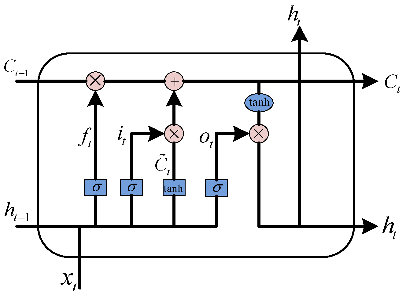
Proposed by Hochreiter Schmidhuber in 1997, the LSTM network [48] is a variant of RNN. Compared with traditional RNN model, it reduces the problem of gradient disappearance by constructing a special neural unit structure, so that the network can use long-distance context information and store knowledge for a long time.
Figure 2 shows the structure of LSTM. The most distinctive feature of LSTM is the usage of gate mechanisms, including a forget gate, input gate and output gate. The input sequence is X = ( x 1 , x 2 , x T ) and then a series of nonlinear mapping functions will be executed and the formulations are as follows
f t = σ ( W f h h t 1 + W f x x t + b f )
i t = σ ( W i h h t 1 + W i x x t + b i )
o t = σ ( W o h h h 1 + W o x x t + b o )
s t = f t s t 1 + i t tanh ( W s h h t 1 + W s x x t + b s )
h t = o t tanh ( s t )
where h t 1 is the previous hidden state, x t is the current input and σ ( ) represents the activation of sigmoid. In addition, f t is the forget gate state, i t is the input gate state, o t is the output gate state, and s t is the memory cell state. Simultaneously, W f , W i , W o , W s and b f , b i , b o , b s are parameters to learn.

3.2. Our Proposed Intelligent System Combining ARIMA and LSTM

Most sequence data in real life involves linear and nonlinear constituents simultaneously, rather than a single constituent. An individual model is not enough to capture complicated relationships between sequences at the same time. Therefore, for the purpose of solving this problem and constructing an accurate system for the POPs concentrations prediction of the Great Lakes, this paper uses intelligent methods to construct an intelligent data analysis system combining ARIMA and LSTM. The architecture of our system is illustrated in Figure 3.
Step 1: Data preprocessing. Before building a system, data preprocessing must be performed on the original data. The quality of data preprocessing will directly affect the performance of the subsequent steps. Our experimental data are derived from the sampling data of POPs concentrations of sites in the Great Lakes region. Usually, due to sampling instrument failure or operator error, there may be abnormal values in the concentration sequence. At this step, abnormal values must be detected and processed. The detailed data preprocessing process will be illustrated in Section 4.2.
Step 2: Construct the optimal ARIMA model. Bayesian Information Criteria (BIC) are used to obtain the optimal parameter values of ARIMA. Since the ARIMA model is good at modeling linear relationships, and the linear predictions can be acquired via this ARIMA model, then the nonlinear residual sequence can be gained correspondingly, according to the following formula
e t = x t L ^ t
where x t is the POPs concentration value, L ^ t is the linear predicted value and e t is the residual error.
Step 3: Construct the first LSTM network to predict the residual sequence. This paper takes the nonlinear external environmental factors such as year, month and season into account. These factors may play an important role to concentration values. After processing, the format of data can be presented by
x ˜ t = ( e t , d 1 , d 2 , d L )
where d l is the external factor. Then, the training data and label data are as follows, and they will be fed into the first LSTM network.
t r a i n X = [ x ˜ 1 x ˜ 2 x ˜ t x ˜ 2 x ˜ 3 x ˜ t + 1 x ˜ n t x ˜ n t + 1 x ˜ n 1 ]
t r a i n Y = [ e t + 1 e t + 2 e t + 3 ]
Furthermore, the optimal parameters of LSTM will be obtained by a grid search, and the nonlinear mapping relationships will be captured between the residual errors and external environmental factors. Then, this model will generate a nonlinear residual prediction sequence N t .
Step 4: Construct the second LSTM network to perceive the mapping relationships between the linear predicted values, nonlinear predictions and true values. The training set is defined by
t r a i n X = [ L 1 N 1 L 2 N 2 L n N n ]
t r a i n Y = [ x 1 x 2 x n ]
This LSTM network will work effectively and generate the final POPs concentrations predictions.
The pseudo-code of our system is presented in Algorithm 1, and the algorithm flow is consistent with the following steps. Firstly, the stationarity of the input series is tested to obtain the value of d of the ARIMA model, and then p and q values are obtained through BIC criterion. The ARIMA model is constructed to obtain linear predictions and residuals. Then, external environmental factors are introduced to construct the first LSTM model to obtain nonlinear residual predictions. Finally, the second LSTM model is constructed to obtain the final POPs concentration predictions. In the pseudo-code, the sequential() method is used to construct a sequential model, the add() method is used to add layers to model, the compile() method is used to compile the built model, the fit() method is used to train data and the predict() method is used to obtain the predictions of the model.
Algorithm 1. Description of algorithm of our system.
Input: x is concentration sequence
Output: predicted values
# Obtain linear predictions from ARIMA model
  ADF(x)
d = 0
while x is not stationary do
x = diff(x)
d = d + 1
end while
  for p in range(1,pmax + 1)
   for q in range(1,qmax + 1)
     model = ARIMA(x,(p,d,q))
     BIC = bic(model)
   end for
  end for
  p,q = Minindex(BIC)
  model = ARIMA(x,(p,d,q))
  L, e = model.predict()    # linear predictions and residuals
# Obtain residual predictions from the first LSTM
  training_set = create_datasets(e,x,d)   # d is external factors
  op = get the optimal hyperparameter using grid search
  model1 = Sequential()
  model1.add(LSTM(op))
  model1.compile(loss = ’mse’, optimizer = ’adam’)
  model1.fit(training_set)
  N = model1.predict()          # residual predictions
# Obtain the predictions from the second LSTM
  training_set1 = create_datasets(N, L)
  op1 = get the optimal hyperparameter using grid search
  model2 = Sequential()
  model2.add(LSTM(op1))
  model2.compile(loss = ’mse’, optimizer = ’adam’)
  model2.fit(training_set1)
  model2.predict()               # predictions

4. Experiments and Performance Analysis

4.1. Datasets

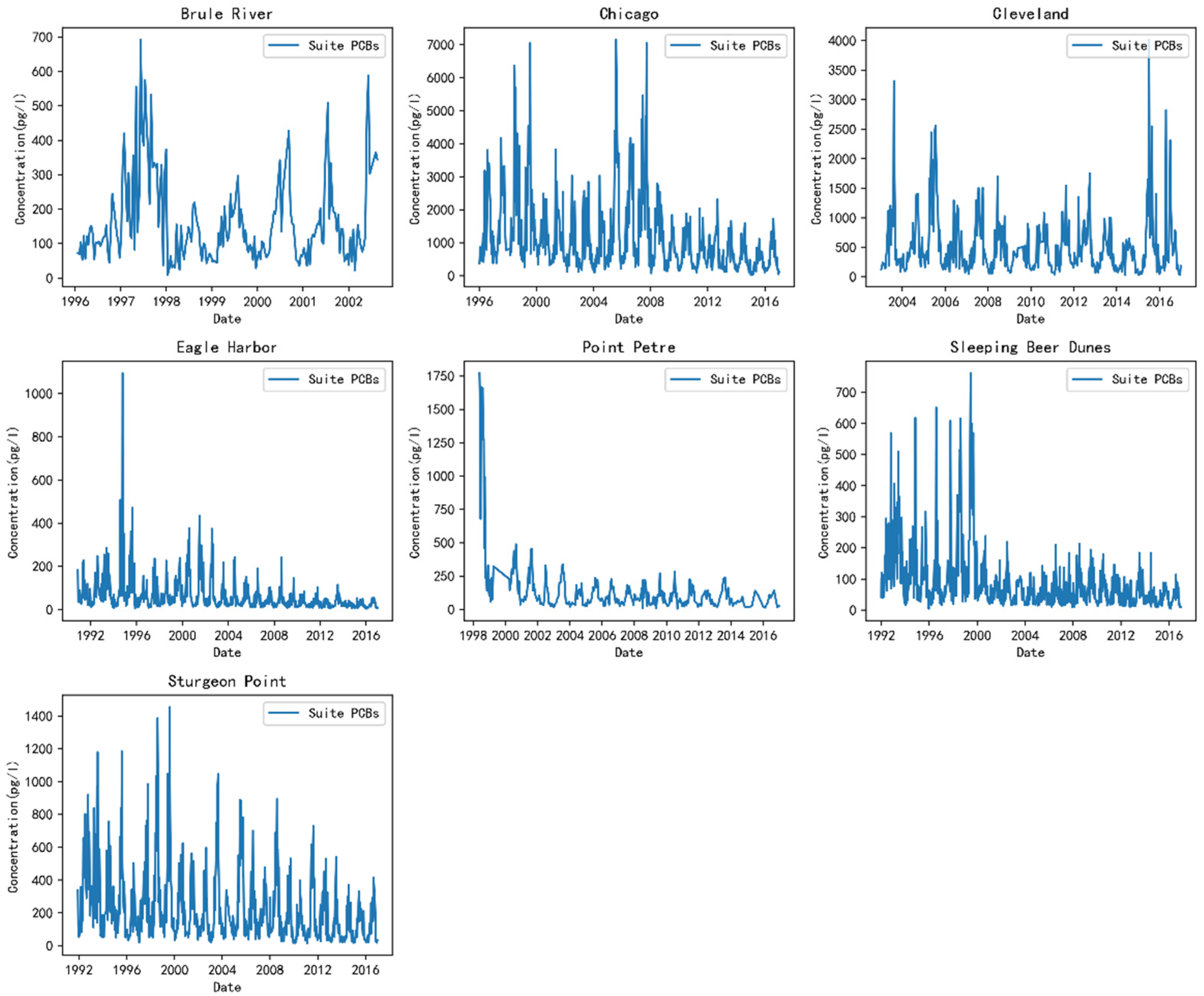
IADN is a collaborative bi-national network of stations that monitor concentrations of persistent toxic chemicals in the phase of air and precipitation in the Great Lakes. Therefore, the data is official, convinced and has extremely high value for research. There are seven monitoring stations in total, Eager Harbor, Brule River, Sleeping Bear Dunes, Sturgeon Point, Point Petre and two satellite stations located in Chicago and Cleveland. These seven sites can be divided into three categories, namely urban sites, rural sites and remote sites. In order to make the experimental data more representative, the monitoring data of Chicago belonging to an urban site, Point Petre belonging to a rural site and Eagle Harbor belonging to a remote site are selected respectively. Moreover, several POPs such as polychlorinated biphenyls (PCBs), organochlorine pesticides (OCs), polycyclic aromatic hydrocarbons (PAHs) and so on were monitored and analyzed at the fixed frequency at these stations. In this paper, we focus on total PCBs concentrations (called Suite PCBs), one of the toxic substances, mainly in vapor phase. Figure 4 is the visualization result of raw data of the Suite PCBs of seven sites. Table 1 details the selected datasets in this paper.

4.2. Data Preprocessing

It can be seen from Figure 4 that the concentrations of PCBs at certain points are abnormally high or low compared to other values, and these points are outliers [49]. Abnormal data, known as outliers, refer to data points that exist in a data set but do not conform to the overall law. In time series data, if the data suddenly change at a certain moment, the data point is likely to be an outlier. If the outliers are not processed reasonably, the accuracy of system will be decreased to a certain extent. Therefore, in the preprocessing stage, performing anomaly detection and fixing outliers are very important. Time series anomaly detection algorithms include statistics-based, distance-based, density-based, cluster-based and tree model-based algorithms. Each algorithm of these categories has their own advantages and disadvantages and is applicable to different scenarios. Patil et al. [50] used PCA for feature extraction to achieve the effect of dimensionality reduction, and then used bidirectional generative adversarial network to detect abnormal network traffic. Binbusayyis et al. [51] adopted an unsupervised deep learning approach, which combined convolutional autoencoder and one-class SVM (OCSVM) for intrusion detection. OCSVM [52], an extension of SVM, is a binary classification method, which is trained using only samples from one class, so it is suitable for unlabeled data. The maximum margin separation between the training points and the original can be found through training, and then the corresponding model can distinguish whether the new data point is a normal value or an outlier. At the same time, the isolation forest [53] is also a commonly used and unsupervised anomaly detection algorithm based on the ensemble method. It requires less time and memory, but it is only sensitive to global outliers, that is to say, it is bad at detecting local outliers. One-class SVM can greatly improve the precision of anomaly detection in the case of small samples, unbalanced sample classification, and supposes no assumptions about data distribution. In view of above discussions, this paper uses the OCSVM method to detect the anomalies of POPs concentration values. Then we use the average sampling concentration in the previous one month to replace this abnormal value. This approach is simple, efficient and can guarantee the authenticity of data to a certain extent.
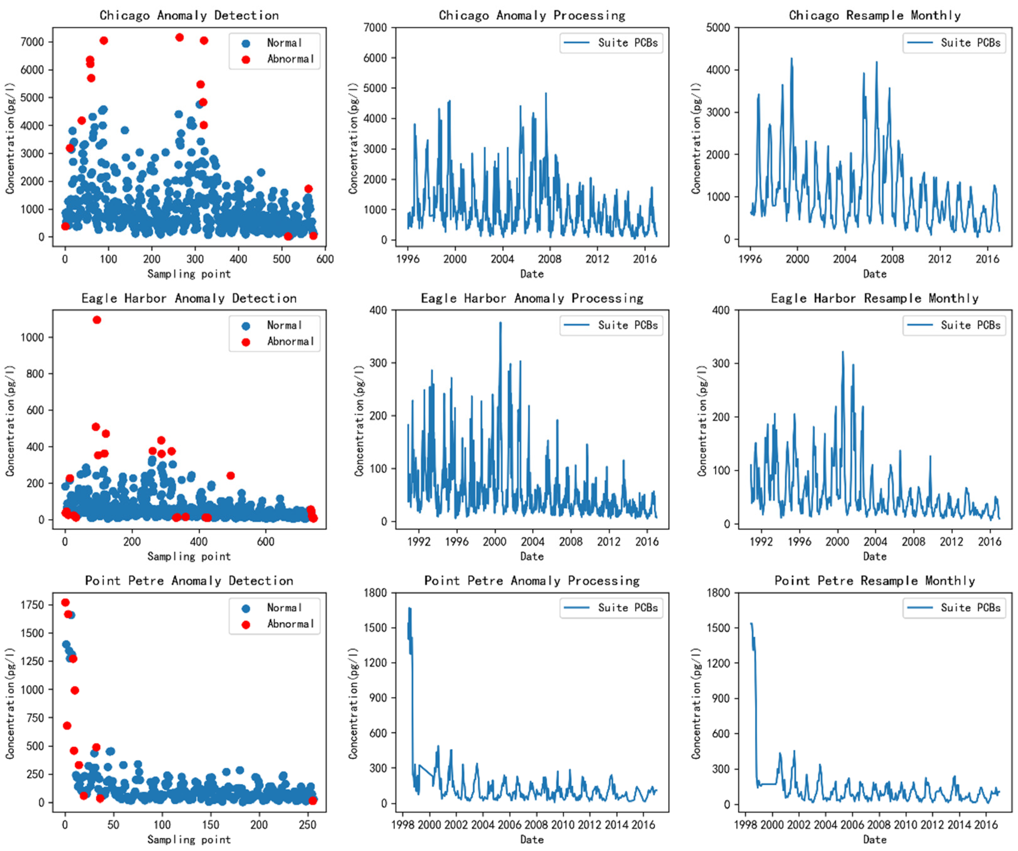
In order to be more suitable for training and prediction of subsequent models, this paper adopts the resampling method to handle data after abnormal processing. Resampling is a commonly used data processing method in statistics [54], which means further processing the current data samples so that the application requirements can be met. Resampling methods in time series domain is the process of converting sequence data from one frequency to another. Converting high-frequency data to low-frequency data is down-sampling, and the reverse is up-sampling. The concentration data were sampled every 12 or 24 days. In order to analyze and predict data more clearly and intuitively, this paper uses down-sampling method to convert the concentration data after abnormal processing into monthly frequency data. That means the average concentration of all sampled values within a month is taken as the concentration value of that month. The results of anomaly detection, processing outliers and resampling monthly in Chicago, Eagle Harbor and Point Petre sites are shown in Figure 5.

4.3. Parameter Tuning

Optimal parameter combination can often greatly improve the performance of model, so it is often essential to look for the optimal parameter combination. The parameter selection process of all models will be introduced in the following subsections.

4.3.1. Parameter Setting for ARIMA

For the ARIMA model, parameters p, d and q should be determined.
  • Determine the value of d. Augmented Dickey Fuller (ADF) test [55] is applied to test the stability of concentration sequence. The essence of ADF test is to judge whether the sequence has a unit root. If sequence is stationary, there is no unit root. If the p-value > 0.05, we cannot reject the null hypothesis (H0) and the sequence has a unit root. Then the subsequent difference operation must be performed. The ADF test was applied to Chicago, Eagle Harbor and Point Petre, respectively, and the results are shown in Table 2. If the ADF statistic value is less than the corresponding Critical Value, then there are, correspondingly, 99%, 95% and 90% probability of rejecting the null hypothesis. However, this paper uses the p-value to determine the value of d. The p-value of Chicago is 0.646, which is greater than 0.05, so a difference operation is required. Similarly, the p-value of Eagle Harbor is 0.363, which is also larger than 0.05, and a difference operation is also required. However, the p-value of Point Petre is 0.001, which is smaller than 0.05, and this series is stationary without difference operation.
  • Determine the parameter order of p and q. The values of p and q are preliminarily determined according to their respective ACF and PACF graphs [55], and then BIC method [56] is used to choose the best parameter order, obtain the minimum value of BIC, and then the corresponding values of p, q are determined.
  • Model evaluation. The test of model is mainly carried out from the following two aspects: Firstly, using the QQ chart [55] to test whether the residual is normally distributed. It can be seen from Figure 6 that the residuals of ARIMA model on the three datasets conform to the normal distribution. Secondly, the D–W (Durbin–Watson) [57] method is used to evaluate the auto-correlation of residuals. The corresponding D–W values are 2.0078, 2.0012, and 1.9988, respectively, which are all close to 2. Hence, there is no auto-correlation of residuals. Finally, the model for Chicago is ARIMA (8,1,3), Eagle Harbor is ARIMA (5,1,3), Point Petre is ARIMA (4,0,2).

4.3.2. Parameter Setting for RNN and LSTM

With the development of deep learning, neural networks have become the latest methods to solve time series problems in recent years. However, obtaining good performance with neural networks is a little difficult, as it involves combinatorial optimizations of hyperparameters, and different hyperparameter values will exert disparate impacts on model performance. There are several important hyperparameters in time series model, i.e., the number of time steps, the number of hidden layers, the number of units of each hidden layer (we set the same units for each layer), batch size and epoch size. To approximate the best performance of model, this paper applies grid search method that is a simple and easily used method to select optimal parameters. The hyperparameters and the search space we tuned are in Table 3. For each combination of hyperparameters, a specified network is trained, and the optimizer is Adam algorithm [58]. Furthermore, the Mean Square Error (MSE) is set as the loss function for all models. The index for selecting the optimal model is Root Mean Square Error (RMSE).
According to the search space of each hyperparameter in Table 3, the RNN and LSTM models are established, respectively, and the hyperparameters are optimized by grid search method. The datasets of Chicago, Eagle Harbor and Point Petre are used to train each model. After extensive experiments, the optimal hyperparameter combinations of RNN and LSTM model on three datasets are obtained, and the results are in Table 4.

4.3.3. Parameter Setting for Our System

The core parts of our intelligent data analysis system are two LSTM networks. The first LSTM network is used to predict nonlinear residual value while adding external nonlinear factors. The second LSTM is used to model linear ARIMA predicted values, nonlinear residual predicted values and true values, and then the final predicted values of our system will be obtained. In Section 4.3.1, the linear prediction values on Chicago, Eagle Harbor and Point Petre datasets have been obtained through ARIMA model, and then the residual values can be obtained by subtracting the linear predictions from true values. Similarly, the optimal hyperparameters of the two LSTM model of our system are obtained by grid search method. The results of hyperparameter selection are shown in Table 5.

4.4. Performance Analysis

To prove the forecasting power of our system, it is compared with three baseline models, namely, ARIMA, RNN and LSTM. The concentration of Suite PCBs at three sites (Chicago site, Eagle Harbor site and Point Petre site) are fitted with these four models. Many experiments are conducted to optimize and train these models. The datasets are split into training set (80%) and testing set (20%) and the performances are separately illustrated as follows.

4.4.1. Evaluation Metrics

For the purpose of analyzing the performance of our system, scientific and effective evaluation criteria should be applied correctly. This paper uses multiple evaluation criteria to estimate the prediction model, including:
Mean Absolute Error (MAE)
MAE = 1 N i = 1 N | y ˜ t i y t i |
Root Mean Square Error (RMSE)
RMSE = 1 N i = 1 N ( y ˜ t i y t i ) 2
Symmetric Mean Absolute Percentage Error (SMAPE)
SMAPE = 100 % N i = 1 N | y ˜ t i y t i | ( | y ˜ t i | + | y t i | ) / 2
where y ˜ t i is predicted value, y t i is actual value and N is the number of samples. All of these indices are widely used in regression tasks. Smaller RMSE and MAE represents better performance, and if SMAPE value is closer to 0, the model’s effect is better.

4.4.2. Chicago Result

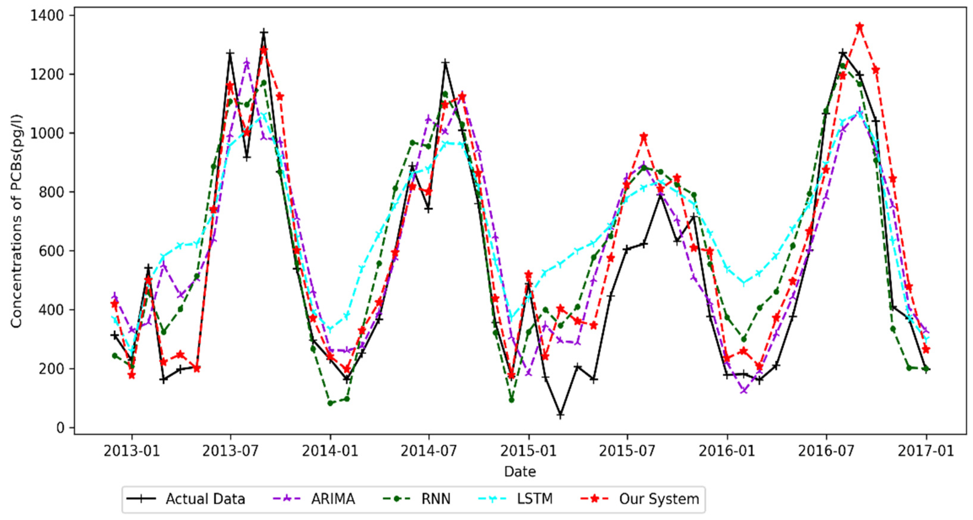
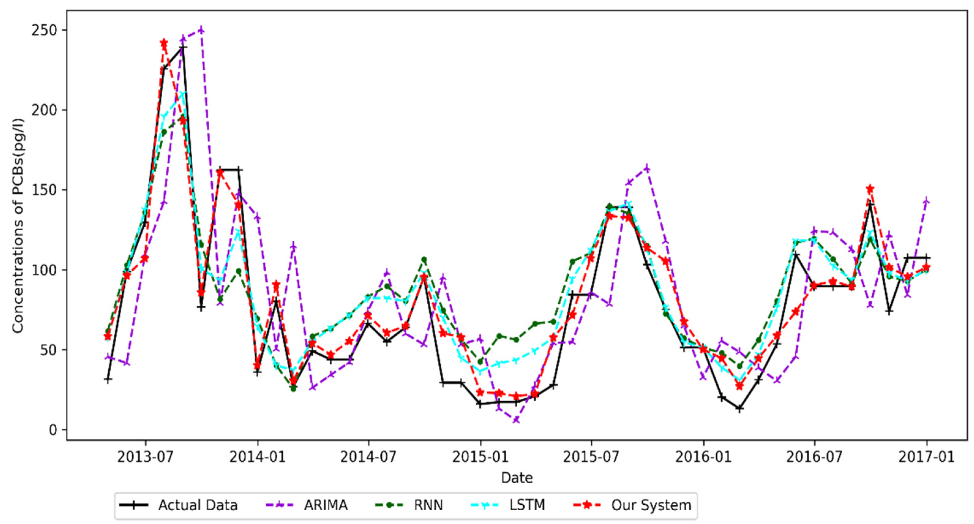
Table 6 shows the results of MAE, RMSE and SMAPE of each model on training set and testing set of Chicago site. On the testing set, the MAE value of RNN model is 139.434, the RMSE value is 166.979 and the SMAPE value is 0.207. Compared with ARIMA and LSTM model, RNN model has better prediction performance. However, our proposed system still shows better prediction accuracy than RNN model. Compared with single model, our proposed system in this paper has the smallest MAE, RMSE and SMAPE on both training set and testing set. The visualization results of predicted values of PCBs concentrations on testing set are shown in Figure 7. It can be noted that the prediction effect of our system is the best. It can not only predict the change trends of PCBs concentrations, but also fit the real concentrations well. The prediction effect of RNN is second and LSTM is the worst.

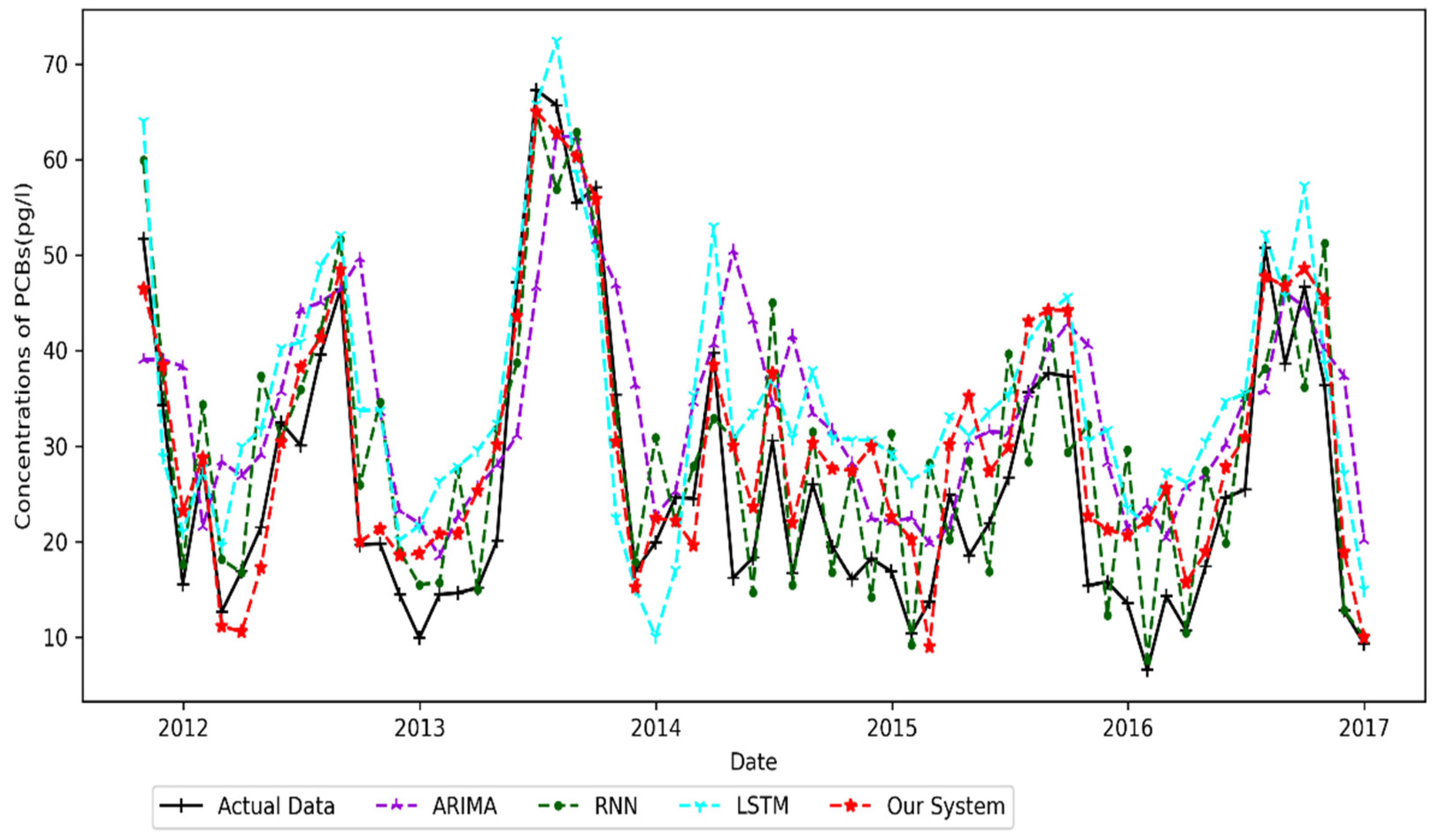
4.4.3. Eagle Harbor Result

Table 7 presents the index values of each prediction model on Eagle Harbor dataset, and Figure 8 shows the fitting curve of each model on testing set. Figure 8 shows a phenomenon that, at the beginning, ARIMA and RNN model have perfect prediction effects, but, over time, the prediction curve of RNN fluctuates greatly. The reason accounting for this phenomenon may be that the relationship between sequence is over-captured. The ARIMA model also cannot predict the change trends of concentrations sequence very well. The reason is that it only learns linear relationships between data. The LSTM model can predict the long-term change trend well, but there is also a certain gap with true values. In comparison, our system shows the best performance in terms of predicting change trend and concentration values. Additionally, our intelligent system has the smallest MAE, RMSE and SMAPE on both training set and testing set. All of these show that our system can still predict well after a period of time.

4.4.4. Point Petre Result

The sampling period of Point Petre was from 1998 to 2016. From the original concentrations diagram in Figure 4, it can be observed that the total concentrations of PCBs in this area have been at a low level. Table 8 shows the predictive performance of each model on dataset. Figure 9 shows the prediction curve of each model on testing set. Figure 9 shows the phenomenon that ARIMA model exhibits the worst fitting effect and has the highest values on MAE, RMSE and SMAPE indicators. From the fitting curve in Figure 9 and index values in Table 8, it can be seen that RNN and LSTM model have similar fitting effects, and both can accurately predict the change trends of concentrations. However, our system has the best predictive performance. On the testing set, its MAE is 10.421, RMSE is 14.726 and SMAPE is 0.087. Additionally, our system can not only predict the trend of concentrations change, but its predictions are very close to the true values. This proves that our system can capture the linear and nonlinear relationships between sequences well, which shows better performance than a single linear or nonlinear model.

4.5. Future Prediction

Based on the historical concentrations measurements, using the intelligent data analysis system proposed in this paper, we predict the concentrations of PCBs in next 5 years of Chicago, Eagle Harbor and Point Petre site, which has critically positive significance for policy formulation, human life, ecosystem environmental protection and sustainability of society. The detailed forecast and analysis results are as follows.

4.5.1. Chicago Prediction Result

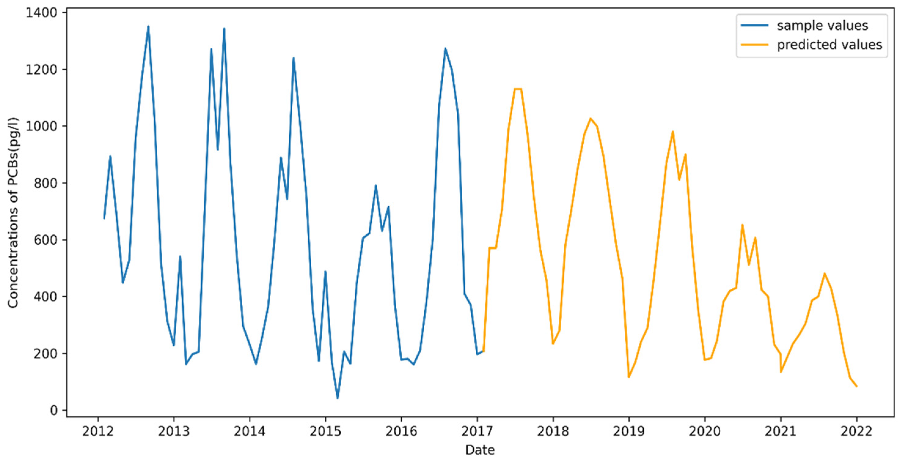
It can be seen from Figure 4 that, from 1996 to 2016, the concentrations of PCBs showed a decreasing trend in general, but among every year there are fluctuations: the concentrations in June, July, August and September reached a high level in a year, and then, in the following months, showed a significant downward trend. All these characteristics show that the concentration values have a strong correlation with environmental factors. Figure 10 presents the predicted values within the next five years that were obtained from our system proposed in this article. It is clear that the concentration values in June, July, August and September of each year are at a higher level, while the other months are at a relatively low level. On the whole, it shows a fluctuating trend that rises firstly and then falls, which shows that our system captures the nonlinear relationship between sequences well.

4.5.2. Eagle Harbor Prediction Result

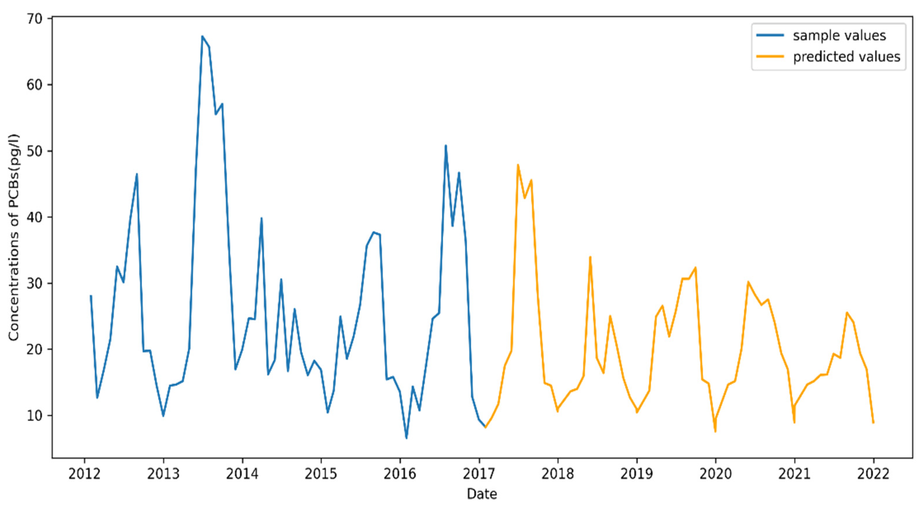
As can be seen from Figure 4, from 1990 to 2016, the total PCBs concentrations at the Eagle Harbor site showed an overall downward trend. After preliminary analysis, the annual average concentration of PCBs in 1990 was 77.59 pg/L, and at the end of 2016 was 24.48 pg/L. The concentration dropped by 53.11 pg/L in 26 years, a 68 percent decline compared with 1990. Although the concentrations of PCBs have shown a downward trend as a whole, they have shown greater fluctuations every year. It can be observed from analysis that the values are at a low level from January to March of each year, and then show a clear upward trend from March to July, and reach the highest level in June or July. After that, there will be an obvious downward trend and it will reach a lower level again in November and December. The predicted concentrations of Eagle Harbor in the following 5 years are shown in Figure 11. It can be seen that the concentration values still show a downward trend in the future, but the fluctuations are still significant every year. By the end of 2021, the annual average concentration is expected to reach 17.19 pg/L, compared with the beginning of 1990, and the rate of decline has reached 77 percent.

4.5.3. Point Petre Prediction Result

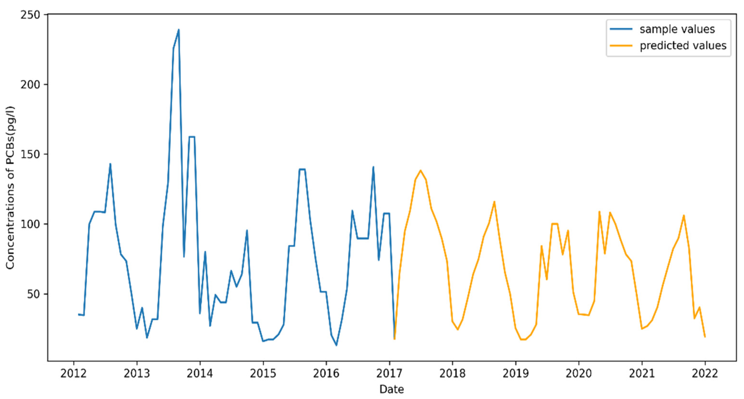
It can be seen from Figure 4 that, from 1998 to 2016, the PCBs concentrations of Point Petre showed a slow downward trend. From 1998 to 2003, the concentrations were at a relatively high level. In 2004, the concentration showed an obvious downward trend, and in the following 10 years, the concentrations were at a relatively stable level with no obvious downward trend. Since 2014, they have shown a slow downward trend. Similar to Chicago and Eagle Harbor site, the concentrations reach the peak from May to August each year and are at a low level in other months. Based on historical concentration observations, our intelligent system combining ARIMA and LSTM is used to predict the total concentrations of PCBs in the next 5 years and the results are presented in Figure 12. From the prediction curve we can note that, in the next 5 years, the PCBs concentrations of Point Petre will show a downward trend, but the decline is still not obvious. At the same time, the concentration values present a fluctuating trend of rising firstly and then falling within each year.

5. Conclusions and Future Work

Based on intelligent methods and data analysis technologies, this paper is dedicated to constructing an intelligent data analysis system to analyze and predict the concentrations of POPs in the Great Lakes region. Considering that the complex concentrations sequence contains linear and nonlinear constituents at the same time and an individual model cannot handle both of them at the same time, this paper combined the ARIMA and LSTM model. In our system, the ARIMA model is used to extract the linear components in the sequence and LSTM is used to capture nonlinear components. Extensive experiments have shown that our intelligent system proposed in this paper shows higher predictive performance than comparison models on experimental datasets. Our intelligent data analysis system can not only predict the concentrations trend more accurately, but also predict the concentrations more accurately. Finally, our system is used to predict the next 5 years concentration values of the Great Lakes region, and the predicted concentrations will show a downward trend on the whole, but there are still great fluctuations in each year.
Our work is critically meaningful to policy formulation, ecological environment protection, the sustainable development of society and so on. This article discusses only one case where the system is used to predict POPs concentrations in the Great Lakes region. However, the application of the work in this paper is not limited, and it can be used to model and analyze other time series data. The computer’s memory requirements of this work depend on the scale of data. If the massive data are to be analyzed, it is necessary to improve the hardware conditions of the computer accordingly. There is still a lot of work to be conducted in the future and this is listed as follows: (1) Although the system shows good prediction performance, there is still a certain gap between predictions and real values, and the accuracy of the system needs to be continuously improved. (2) Consider constructing a fully automated predicting forecasting system to obtain accurate predictions intelligently without human interventions. (3) The system in this paper should be popularized vigorously in the application of pollutants prediction and other time series prediction.

Author Contributions

Conceptualization, C.W.; methodology, L.Y. and C.W.; software, L.Y.; validation, L.Y.; formal analysis, C.W. and L.Y.; investigation, N.N.X.; resources, C.W. and N.N.X.; data curation, L.Y.; writing—original draft preparation, L.Y.; writing—review and editing, L.Y.; visualization, L.Y.; supervision, C.W. and N.N.X. All authors have read and agreed to the published version of the manuscript.

Funding

This research was funded by the National Key Research and Development Program of China (Nos. 2018YFC0810204 and 2018YFB17026), National Natural Science Foundation of China (No. 61872242), Shanghai Science and Technology Innovation Action Plan Project (17511107203), and Shanghai key lab of modern optical system.

Data Availability Statement

All original POPs concentration data of Great Lakes can be found in https://iadnviz.iu.edu/about/index.html (accessed on 1 January 2021) and process data in this study are available from the corresponding author.

Acknowledgments

The authors would like to appreciate all anonymous reviewers for their insightful comments and constructive suggestions to polish this paper to its highest quality.

Conflicts of Interest

The authors declare no conflict of interest.

References

  1. Magulova, K.; Priceputu, A. Global monitoring plan for persistent organic pollutants (POPs) under the Stockholm Convention: Triggering, streamlining and catalyzing global POPs monitoring. Environ. Pollut. 2016, 217, 82–84. [Google Scholar] [CrossRef] [PubMed]
  2. Zheng, M.; Tan, L.; Gao, L.; Ma, L.; Dong, S.; Yao, Y. Global Monitoring Plan of POPs Under the Stockholm Convention for Effectivenes Evaluation. Environ. Monit. China 2019, 35, 6–12. [Google Scholar]
  3. Ping, S.; Basu, I.; Blanchard, P.; Backus, S.M.; Hites, R.A. Temporal and Spatial Trends of Atmospheric Toxic Substances near the Great Lakes IADN Results Through 2003; Environment Canada and the United States Environmental Protection Agency: Chicago, IL, USA, 2002.
  4. Xia, F.; Hao, R.; Li, J.; Xiong, N.; Yang, L.T.; Zhang, Y. Adaptive GTS allocation in IEEE 802.15.4 for real-time wireless sensor networks. J. Syst. Archit. 2013, 59, 1231–1242. [Google Scholar] [CrossRef]
  5. Akyildiz, I.F.; Su, W.; Sankarasubramaniam, Y.; Cayirci, E. A Survey on Sensor Networks. IEEE Commun. Mag. 2002, 40, 102–114. [Google Scholar] [CrossRef] [Green Version]
  6. Gao, K.; Han, F.; Dong, P.; Xiong, N.; Du, R. Connected Vehicle as a Mobile Sensor for Real Time Queue Length at Signalized Intersections. Sensors 2019, 19, 2059. [Google Scholar] [CrossRef] [PubMed] [Green Version]
  7. Huang, S.; Liu, A.; Wang, T.; Xiong, N.N. BD-VTE: A Novel Baseline Data based Verifiable Trust Evaluation Scheme for Smart Network Systems. IEEE Trans. Netw. Sci. Eng. 2020, 8, 2087–2105. [Google Scholar] [CrossRef]
  8. Baothman, F.A. An Intelligent Big Data Management System Using Haar Algorithm-Based Nao Agent Multisensory Communication. Wirel. Commun. Mob. Comput. 2021, 2021, 9977751. [Google Scholar] [CrossRef]
  9. Yao, Y.; Xiong, N.; Park, J.H.; Ma, L.; Liu, J. Privacy-preserving max/min query in two-tiered wireless sensor networks. Comput. Math. Appl. 2013, 65, 1318–1325. [Google Scholar] [CrossRef]
  10. Wu, M.; Tan, L.; Xiong, N. A Structure Fidelity Approach for Big Data Collection in Wireless Sensor Networks. Sensors 2014, 15, 248. [Google Scholar] [CrossRef] [Green Version]
  11. Berthold, M.R.; Borgelt, C.; Höppner, F.; Klawonn, F. Intelligent Data Analysis; Springer: Berlin, Germany, 1999. [Google Scholar]
  12. Box, G.; Jenkins, G. Time Series Analysis Forecasting and Control. J. Time Ser. Anal. 1970, 3, 131–133. [Google Scholar]
  13. Jiang, Y.; Tong, G.; Yin, H.; Xiong, N. A Pedestrian Detection Method Based on Genetic Algorithm for Optimize XGBoost Training Parameters. IEEE Access 2019, 7, 118310–118321. [Google Scholar] [CrossRef]
  14. Paula, A.J.; Ferreira, O.P.; Filho, A.G.S.; Filho, F.N.; Andrade, C.E.; Faria, A.F. Machine Learning and Natural Language Processing Enable a Data-Oriented Experimental Design Approach for Producing Biochar and Hydrochar from Biomass. Chem. Mater. 2022, 34, 979–990. [Google Scholar] [CrossRef]
  15. He, R.; Xiong, N.; Yang, L.T.; Park, J.H. Using Multi-Modal Semantic Association Rules to fuse keywords and visual features automatically for Web image retrieval. Inf. Fusion 2011, 12, 223–230. [Google Scholar] [CrossRef]
  16. Li, H.; Liu, J.; Wu, K.; Yang, Z.; Liu, R.W.; Xiong, N. Spatio-Temporal Vessel Trajectory Clustering Based on Data Mapping and Density. IEEE Access 2018, 6, 58939–58954. [Google Scholar] [CrossRef]
  17. Wang, Y.; Li, Y.; Sui, J.; Gao, Y. Data Factory: An Efficient Data Analysis Solution in the Era of Big Data. In Proceedings of the 2020 5th IEEE International Conference on Big Data Analytics (ICBDA), Xiamen, China, 8–11 May 2020. [Google Scholar]
  18. Wang, Z.; Li, T.; Xiong, N.; Pan, Y. A novel dynamic network data replication scheme based on historical access record and proactive deletion. J. Supercomput. 2012, 62, 227–250. [Google Scholar] [CrossRef]
  19. Yang, P.; Xiong, N.N.; Ren, J. Data Security and Privacy Protection for Cloud Storage: A Survey. IEEE Access 2020, 8, 131723–131740. [Google Scholar] [CrossRef]
  20. Dien, N.T.; Hirai, Y.; Koshiba, J.; Sakai, S.I. Factors affecting multiple persistent organic pollutant concentrations in the air above Japan: A panel data analysis. Chemosphere 2021, 277, 130356. [Google Scholar] [CrossRef]
  21. Guo, W.; Xiong, N.; Vasilakos, A.V.; Chen, G.; Cheng, H. Multi-Source Temporal Data Aggregation in Wireless Sensor Networks. Wirel. Pers. Commun. 2011, 56, 359–370. [Google Scholar] [CrossRef]
  22. Yin, J.; Lo, W.; Deng, S.; Li, Y.; Wu, Z.; Xiong, N. Colbar: A collaborative location-based regularization framework for QoS prediction. Inf. Sci. Int. J. 2014, 265, 68–84. [Google Scholar] [CrossRef]
  23. Simcik, M.F.; Basu, I.; Sweet, C.W.; Hites, R.A. Temperature Dependence and Temporal Trends of Polychlorinated Biphenyl Congeners in the Great Lakes Atmosphere. Environ. Sci. Technol. 1999, 33, 1991–1995. [Google Scholar] [CrossRef]
  24. Sun, P.; Basu, I.; Hites, R.A. Temporal trends of polychlorinated biphenyls in precipitation and air at Chicago. Environ. Sci. Technol. 2006, 40, 1178. [Google Scholar] [CrossRef] [PubMed]
  25. Hites, R.A. Statistical Approach for Assessing the Stockholm Convention’s Effectiveness: Great Lakes Atmospheric Data. Environ. Sci. Technol. 2019, 53, 8585–8590. [Google Scholar] [CrossRef] [PubMed]
  26. Venier, M.; Salamova, A.; Hites, R.A. Temporal trends of persistent organic pollutant concentrations in precipitation around the Great Lakes. Environ. Pollut. 2016, 217, 143–148. [Google Scholar] [CrossRef] [PubMed]
  27. Zhao, Y. Statistical Analysis of Climate Change Signals in Typical Persistent Organic Pollutants in the Arctic and Great Lakes Regions. Ph.D. Thesis, Lanzhou University, Lanzhou, China, 2017. [Google Scholar]
  28. Yuan, Q. Prediction of Air/Particulate Matter Partition Coefficient (K_p) for Some Persistent Organic Pollutants; Zhejiang Normal University: Jinhua, China, 1956. [Google Scholar]
  29. Jones, K.C. Persistent Organic Pollutants (POPs) and Related Chemicals in the Global Environment: Some Personal Reflections. Environ. Sci. Technol. 2021, 55, 9400–9412. [Google Scholar] [CrossRef]
  30. Girones, L.; Oliva, A.L.; Negrin, V.L.; Marcovecchio, J.E.; Arias, A.H. Persistent organic pollutants (POPs) in coastal wetlands: A review of their occurrences, toxic effects, and biogeochemical cycling. Mar. Pollut. Bull. 2021, 172, 112864. [Google Scholar] [CrossRef]
  31. Zhang, Q.; Zhou, C.; Tian, Y.C.; Xiong, N.; Qin, Y.; Hu, B. A Fuzzy Probability Bayesian Network Approach for Dynamic Cybersecurity Risk Assessment in Industrial Control Systems. IEEE Trans. Ind. Inform. 2018, 14, 2497–2506. [Google Scholar] [CrossRef] [Green Version]
  32. Zhu, T.; Tao, C. Prediction models with multiple machine learning algorithms for POPs: The calculation of PDMS-air partition coefficient from molecular descriptor. J. Hazard. Mater. 2021, 423, 127037. [Google Scholar] [CrossRef]
  33. Das, M.; Ghosh, S.K. A probabilistic approach for weather forecast using spatio-temporal inter-relationships among climate variables. In Proceedings of the 2014 9th International Conference on Industrial and Information Systems (ICIIS), Gwalior, India, 15–17 December 2014; IEEE: Manhattan, NY, USA, 2014. [Google Scholar]
  34. Mellit, A.; Pavan, A.M.; Benghanem, M. Least squares support vector machine for short-term prediction of meteorological time series. Theor. Appl. Climatol. 2013, 111, 297–307. [Google Scholar] [CrossRef]
  35. Wu, C.; Wang, C.; Fan, Q.; Wu, Q.; Xu, S.; Xiong, N.N. Design and Analysis of an Data-Driven Intelligent Model for Persistent Organic Pollutants in the Internet of Things Environments. IEEE Access 2021, 9, 13451–13463. [Google Scholar] [CrossRef]
  36. Alabdulrazzaq, H.; Alenezi, M.N.; Rawajfih, Y.; Alghannam, B.A.; Al-Hassan, A.A.; Al-Anzi, F.S. On the accuracy of ARIMA based prediction of COVID-19 spread. Results Phys. 2021, 27, 104509. [Google Scholar] [CrossRef]
  37. Zhao, Y.; Wang, L.; Luo, J.; Huang, T.; Ma, J. Deep Learning Prediction of Polycyclic Aromatic Hydrocarbons in the High Arctic. Environ. Sci. Technol. 2019, 53, 13238–13245. [Google Scholar] [CrossRef] [PubMed]
  38. Abbasimehr, H.; Shabani, M.; Yousefi, M. An optimized model using LSTM network for demand forecasting. Comput. Ind. Eng. 2020, 143, 106435. [Google Scholar] [CrossRef]
  39. Wu, C.; Li, B.; Xiong, N. An Effective Machine Learning Scheme to Analyze and Predict the Concentration of Persistent Pollutants in the Great Lakes. IEEE Access 2021, 9, 52252–52265. [Google Scholar] [CrossRef]
  40. Phan, T.; Hoai, N.X. Combining Statistical Machine Learning Models with ARIMA for Water Level Forecasting: The Case of the Red River. Adv. Water Resour. 2020, 142, 103656. [Google Scholar] [CrossRef]
  41. Xu, G.; Cheng, Y.; Liu, F.; Ping, P.; Sun, J. A Water Level Prediction Model Based on ARIMA-RNN. In Proceedings of the 2019 IEEE Fifth International Conference on Big Data Computing Service and Applications (BigDataService), San Francisco, CA, USA, 4–9 April 2019. [Google Scholar]
  42. Kim, T.Y.; Cho, S.B. Predicting Residential Energy Consumption using CNN-LSTM Neural Networks. Energy 2019, 182, 72–81. [Google Scholar] [CrossRef]
  43. Xiaofei, Y.; Qiming, Y.; Xingchen, Y.; Tao, W.; Jun, C.; Song, L. Demand Forecasting of Online Car-Hailing with Combining LSTM + Attention Approaches. Electronics 2021, 10, 2480. [Google Scholar]
  44. Fang, W.; Zhu, R. Air quality prediction model based on spatial-temporal similarity LSTM. Appl. Res. Comput. 2021, 38, 2640–2645. [Google Scholar] [CrossRef]
  45. Li, Y.; Zhu, Z.; Kong, D.; Hua, H.; Yao, Z. EA-LSTM: Evolutionary Attention-based LSTM for Time Series Prediction. Knowl. Based Syst. 2018, 181, 104785. [Google Scholar] [CrossRef] [Green Version]
  46. Liang, Y.; Ke, S.; Zhang, J.; Yi, X.; Yu, Z. GeoMAN: Multi-level Attention Networks for Geo-sensory Time Series Prediction. In Proceedings of the Twenty-Seventh International Joint Conference on Artificial Intelligence {IJCAI-18}, Freiburg, Germany, 13–19 July 2018. [Google Scholar]
  47. Rumelhart, D.; Hinton, G.E.; Williams, R.J. Learning Representations by Back Propagating Errors. Nature 1986, 323, 533–536. [Google Scholar] [CrossRef]
  48. Graves, A. Long Short-Term Memory; Springer: Berlin/Heidelberg, Germany, 2012. [Google Scholar]
  49. Blázquez-García, A.; Conde, A.; Mori, U.; Lozano, J.A. A review on outlier/anomaly detection in time series data. ACM Comput. Surv. 2020, 54, 1–33. [Google Scholar] [CrossRef]
  50. Patil, R.; Biradar, R.; Ravi, V.; Biradar, P.; Ghosh, U. Network traffic anomaly detection using PCA and BiGAN. Internet Technol. Lett. 2022, 5, e235. [Google Scholar] [CrossRef]
  51. Binbusayyis, A.; Vaiyapuri, T. Unsupervised deep learning approach for network intrusion detection combining convolutional autoencoder and one-class SVM. Appl. Intell. 2021, 51, 7094–7108. [Google Scholar] [CrossRef]
  52. Olkopf, B.S.; Williamson, R.; Smola, A.; Shawe-Taylor, J.; Platt, J. Support Vector Method for Novelty Detection. In Proceedings of the Advances in Neural Information Processing Systems, Cambridge, MA, USA, 7 April 2000. [Google Scholar]
  53. Fei, T.L.; Kai, M.T.; Zhou, Z.H. Isolation Forest. In Proceedings of the IEEE International Conference on Data Mining, Washington, DC, USA, 15–19 December 2008. [Google Scholar]
  54. Guo, H.; Li, Y.; Js, D.; Gu, M.A.; Huang, Y.A.; Gong, B.E. Learning from class-imbalanced data: Review of methods and applications. Expert Syst. Appl. 2017, 73, 220–239. [Google Scholar]
  55. Otnes, R.K.; Enochson, L.; Maqusi, M. Applied Time Series Analysis, Vol. 1. IEEE Trans. Syst. Man Cybern. 1981, 11, 292–293. [Google Scholar] [CrossRef]
  56. De, H.; Acquah, G. Comparison of Akaike information criterion (AIC) and Bayesian information criterion (BIC) in selection of an asymmetric price relationship. J. Dev. Agric. Econ. 2010, 2, 1–6. [Google Scholar]
  57. Yang, W. Time Series Analysis and Dynamic Data Modeling; Beijing Institute of Technology Press: Beijing, China, 1986. [Google Scholar]
  58. Kingma, D.; Ba, J. Adam: A Method for Stochastic Optimization. In Proceedings of the 3rd International Conference on Learning Representations, ICLR 2015, San Diego, CA, USA, 7–9 May 2015. [Google Scholar]
Figure 1. Recurrent neural network structure.
Electronics 11 00652 g001
Figure 2. Long short-term memory network structure.
Electronics 11 00652 g002
Figure 3. The architecture of our intelligent data analysis system combining ARIMA and LSTM.
Electronics 11 00652 g003
Figure 4. Visualization of original concentration values of Suite PCBs at seven monitoring stations in Great Lakes region.
Electronics 11 00652 g004
Figure 5. Anomaly detection, anomaly processing and monthly resampling results of three sites.
Electronics 11 00652 g005
Figure 6. QQ plots of ARIMA model for three sites.
Electronics 11 00652 g006
Figure 7. Prediction results of each model on Chicago dataset.
Electronics 11 00652 g007
Figure 8. Prediction results of each model on Eagle Harbor dataset.
Electronics 11 00652 g008
Figure 9. Prediction results of each model on Point Petre dataset.
Electronics 11 00652 g009
Figure 10. The predicted concentration values of PCBs at Chicago in the next 5 years.
Electronics 11 00652 g010
Figure 11. The predicted concentration values of PCBs at Eagle Harbor in the next 5 years.
Electronics 11 00652 g011
Figure 12. The predicted concentration values of PCBs at Point Petre in the next 5 years.
Electronics 11 00652 g012
Table 1. Details of experimental datasets.
SitePeriodFrequencyNumber of SamplesSite Type
Chicago1996–201612 days574urban site
Eagle Harbor1990–201612 days744remote site
Point Petre1998–201624 days257rural site
Table 2. ADF test.
Table 2. ADF test.
ChicagoEagle HarborPoint Petre
ADF Statistic−1.263−1.835−4.019
p-value0.6460.3630.001
Critical Value 1%−3.458−3.452−3.462
Critical Value 5%−2.874−2.871−2.875
Critical Value 10%−2.573−2.572−2.574
Table 3. Hyperparameters and their specific search space.
HyperparameterSearch Space
Time step(1, 2, 3, 4, 5, 6, 7, 8, 9, 10, 11, 12)
The number of hidden layers(1, 2, 3)
The number of units(8, 16, 32, 64, 128)
Batch size(1, 4, 8)
Epoch size(50, 100, 150, 200)
Table 4. The optimal hyperparameter combination of RNN and LSTM model on three sites.
HyperparameterChicagoEagle HarborPoint Petre
RNNLSTMRNNLSTMRNNLSTM
Time Step865544
The number of hidden layers122221
The number of units32168323264
Batch size1111111
Epoch size10050100200100150
Table 5. Optimal hyperparameter combination of our system on three sites.
HyperparameterChicagoEagle HarborPoint Petre
The First LSTMThe Second LSTMThe First LSTMThe Second LSTMThe First LSTMThe Second LSTM
Time Step664546
The number of hidden layers212322
The number of units832168648
Batch size111111
Epoch size100501001505050
Table 6. Comparison of index values of each model on Chicago dataset.
MethodTraining SetTesting Set
MAERMSESMAPEMAERMSESMAPE
ARIMA384.961533.9940.324166.580199.3530.319
RNN376.999526.7460.185139.434166.9790.207
LSTM392.453549.7710.358201.262242.3280.323
Our System205.010350.3250.104110.279143.9140.102
Table 7. Comparison of index values of each model on Eagle Harbor dataset.
MethodTraining SetTesting Set
MAERMSESMAPEMAERMSESMAPE
ARIMA26.34338.9530.3065.6136.6670.249
RNN27.11646.0470.3737.88910.4250.297
LSTM20.37730.1390.1689.889.750.112
Our System15.44420.1980.0844.0135.6670.092
Table 8. Comparison of index values of each model on Point Petre dataset.
MethodTraining SetTesting Set
MAERMSESMAPEMAERMSESMAPE
ARIMA56.49493.6320.27236.53048.6860.299
RNN47.30565.8270.20823.98129.4900.173
LSTM47.03270.6490.20618.97523.1960.161
Our System29.93944.2210.10510.42114.7260.087
Publisher’s Note: MDPI stays neutral with regard to jurisdictional claims in published maps and institutional affiliations.