
Methodology to Differentiate Legume Species in Intercropping Agroecosystems Based on UAV with RGB Camera


Abstract
:1. Introduction
2. Materials and Methods
2.1. Study Site
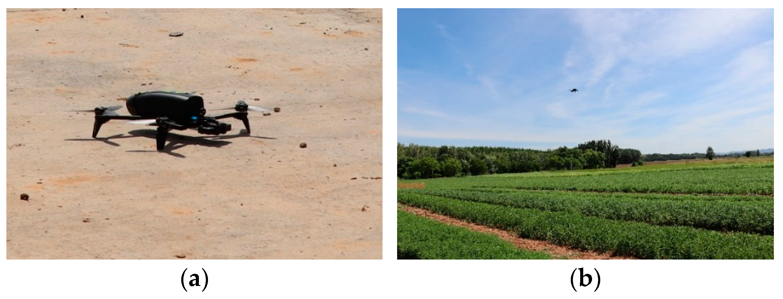
2.2. Image Gathering
2.3. Image Classification Process
- The first step is to obtain the Soil Index (SI) and the Vegetation Index (VI), defined in [18].
- After obtaining the output of both indices (SI and VI), the mathematical combination of both indices is performed to obtain the Vegetation–Soil Index (VSI). To do so, the first step is to reclassify the data of SI to generate a mask. The rule for the reclassification is the following one: if the original pixel value = 0, the newly assigned value is 0. If the original pixel value = “Else”, the newly assigned value is 1. The objective of this soil mask, or Reclassified SI (rSI), is to reduce the variability of soil pixel values in the VI to simplify the reclassification of the results after the aggregation.
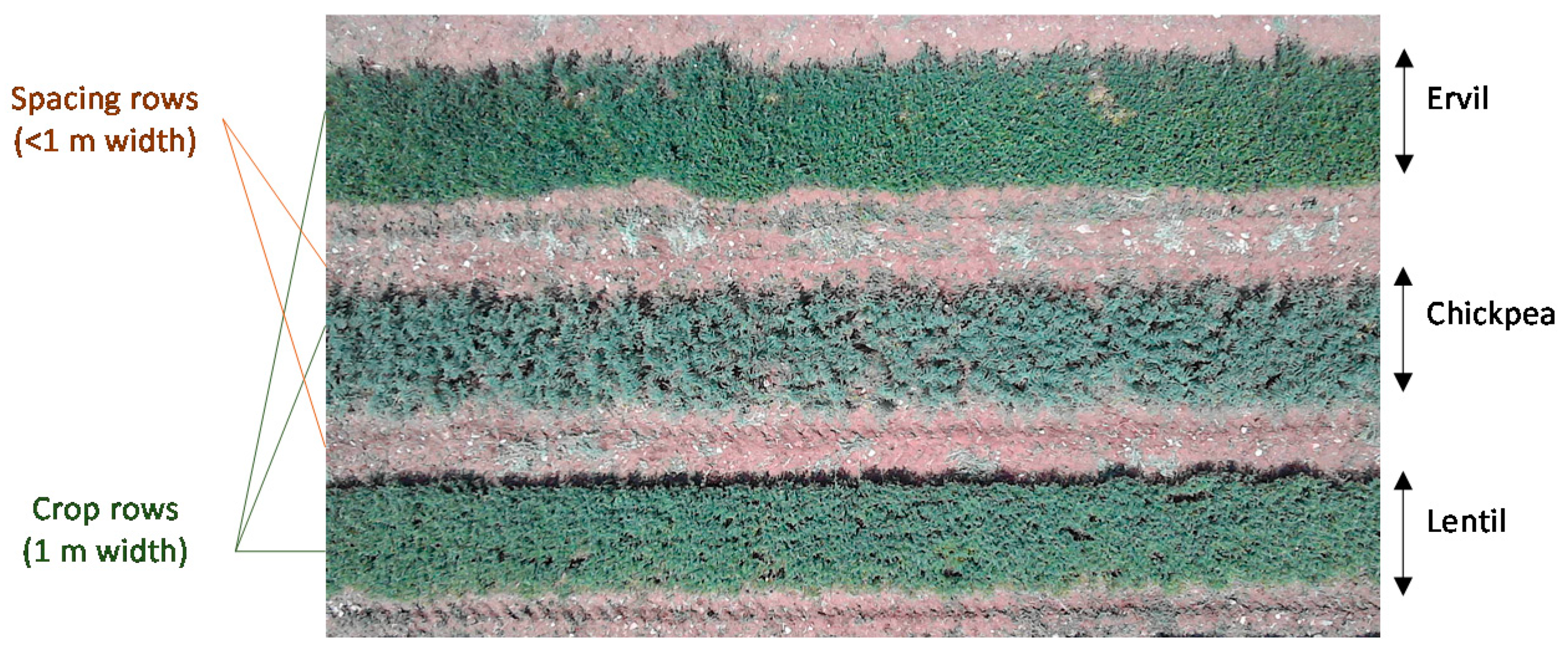
- The next step is to aggregate the VSI to generate the Aggregated VSI (VSIA). The aggregation is performed to reduce the size of the picture and minimize the effect of isolated pixels, which usually represent abnormal values. For this, the operator must be selected in the “beyond node process”. The selected operator will be applied to the VSI with a cell size of 20 pixels. The cell size of 20 was set to ensure a minimum width of 8 pixels for each crop row in the images captured at 16 m.
- Once the VSIA is obtained, the soil mask (the rSI) is applied again, generating the Masked VSIA (VSIAM) to ensure that all soil pixels have a value of 0.
- The subsequent step is the reclassification in 5 classes and obtaining the Reclassified VSIAM (rVSIAM). In this step, the values used for the classification are defined according to the results of thresholds generation in the “beyond node process”.
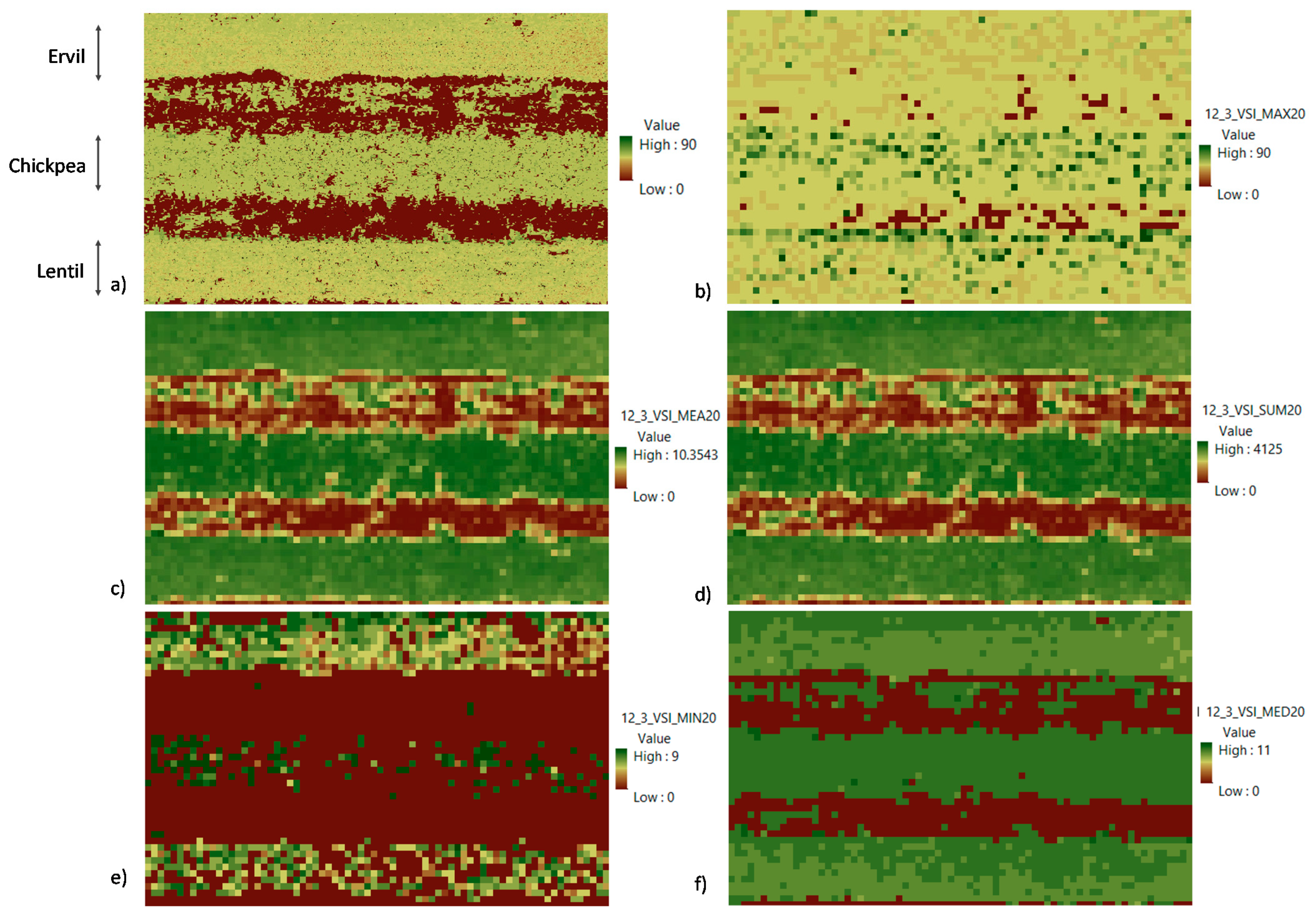
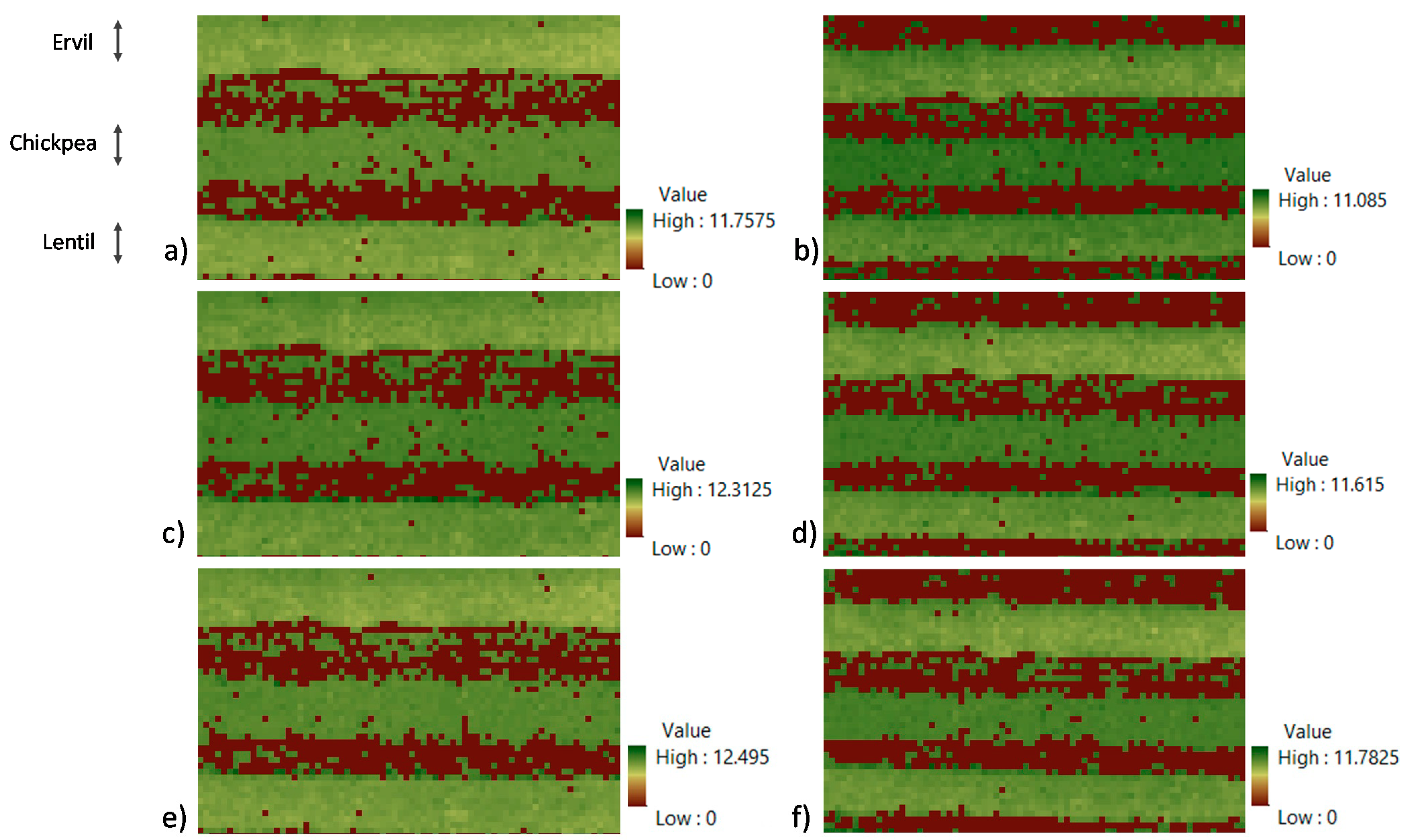
- The first step is to compare the best operator for aggregation of the VSI. The five operators (maximum, summation, mean, median and minimum) are compared for that purpose. The resultant aggregated VSI are compared, first visually, and then by comparing the variance of the three crop rows. In the first comparison the worthless results are excluded. Worthless results are the aggregated images in which the different crop lines cannot be identified or those with the same values. The second comparison extracts each crop row’s mean, maximum, minimum, and standard deviation (σ). After normalizing the data, each crop line’s minimum and maximum values are compared, and the operator that offers the greater variability between crops (inter-crop variability) is selected. If the operators showed similar inter-crop variability, the one with the greater intra-crop variability is selected.
- The next step is the attainment of thresholds for the VSIAM. The initial procedure is to analyze whether it is feasible to distinguish crop type. Therefore, the histograms of each crop row are obtained and mean values are compared with an ANalysis Of VAriance (ANOVA). Once ANOVA identifies whether data can be used to differentiate the crops, unsupervised classification methods are used to generate a variable number of classes. Then, the classes are merged in a supervised classification to attain the thresholds.
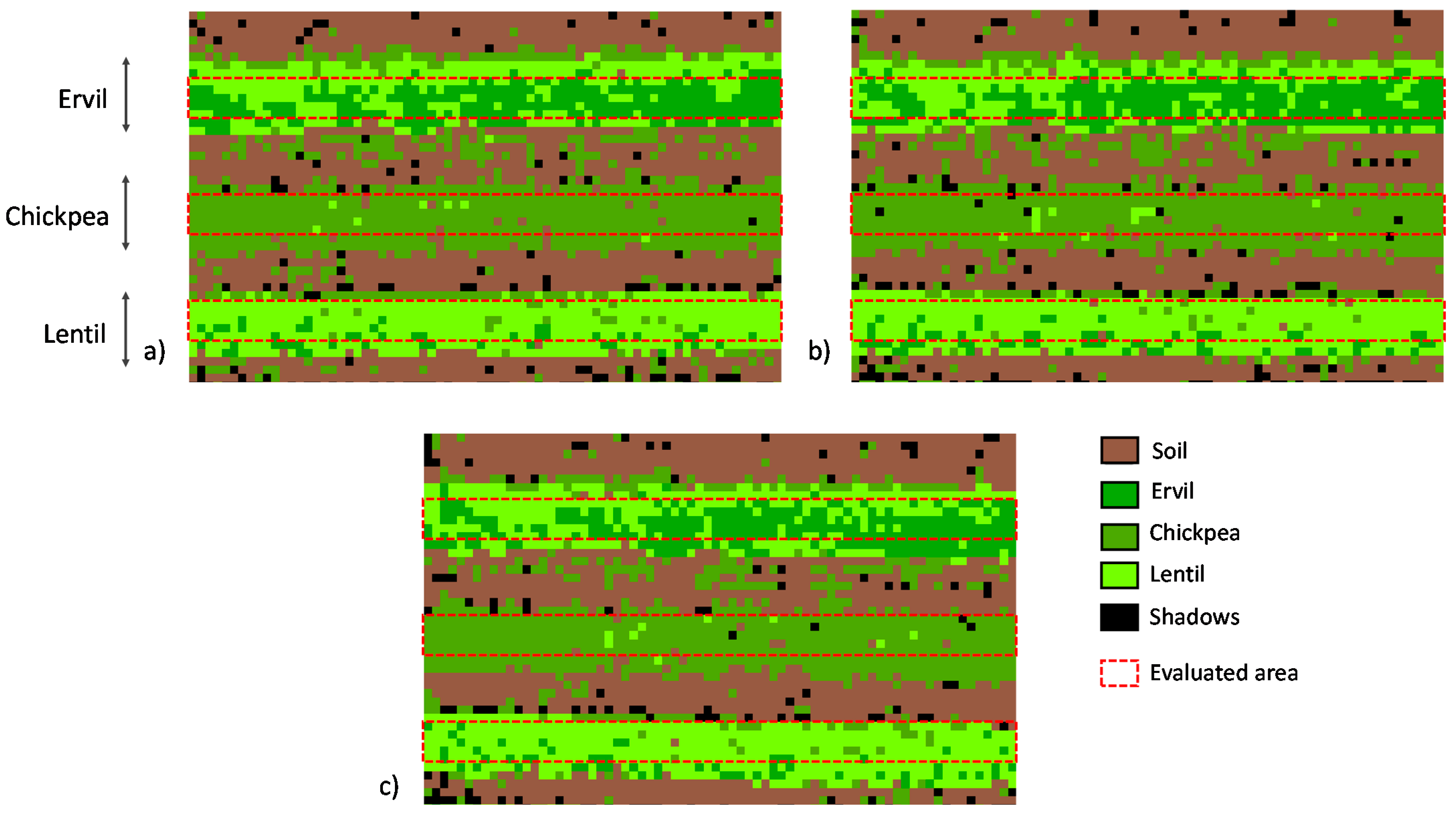
- Finally, the evaluation of the accuracy of rVSIAM is performed. Three areas that contain the majority of each crop row are analyzed to determine the accuracy according to the initial crop type and the classified crop type.
| Algorithm 1: The Code for Aggregate Operation |
| # Code for Aggregate Operation import arcpy from arcpy import env from arcpy.sa import * env.workspace = “C:/sapyexamples/data” outAggreg = Aggregate(“VSI”, 20, “SUMMATION”, “TRUNCATE”, “DATA”) outAggreg.save(“C:/sapyexamples/output/VSIa” |
| Algorithm 2: The Code for Reclassify Operation |
| # Code for Reclassify Operation import arcpy from arcpy import env from arcpy.sa import * env.workspace = “C:/sapyexamples/data” outReclass1 = Reclassify(“VSIam”, “Value”, RemapRange ([[0,1], [0,a,2], [a,b,2], [b,c,3], [c,d,4], [d,e,5]])) outReclass1.save(“C:/sapyexamples/output/rVSIam”) |
3. Results
3.1. Application of Vegetation and Soil Indices
3.2. Selection of Best Aggregation Technique
3.3. Classification of Crops
3.3.1. Crop Types Differentiation
3.3.2. Crop Types Classification
4. Discussion
4.1. Comparison of Results with Literature

| Management | Crop/s | Source | Approach | Accuracy | Ref | ||
|---|---|---|---|---|---|---|---|
| Global | Min. | Max. | |||||
| Mono-crop in heterogeneous mosaic | Alfalta, Almond, Walnut, Vineyards, Corn, Rice, Safflower, Sunflower, Tomato, Meadow, Oat, Rye, and Wheat | ASTER satellite (3 sampling periods) | OBIA | 80 | 69 | 100 | [21] |
| Mono-crop in heterogeneous mosaic | Winter cereal stubble, Vineyards, Olive orchards, and Spring-sown sunflowers | QuickBird | OBIA | - | 16 | 100 | [22] |
| Mono-crop in heterogeneous mosaic | Rice, Greenhouse, Corn, Tree, Unripe wheat, Ripe wheat, Grassland, and Soybean | UAV (RGB camera) + DSM data | SVM | 72.94 * 94.5 ** | - | - | [23] |
| Mono-crop in heterogeneous mosaic | Grassland, Ginsen, Vinly house, Barren Paddy, Radish, and Chinese cabbage | UAV (RGB camera) | OBIA | 85 | 68 | 100 | [24] |
| Heterogeneous mosaic with mono-crop and intercrop (legumes) | Banana, Legumes, and Maize | UAV (RGB camera) | DNN | 86 | 49 | 96 | [14] |
| Mono-crop in heterogeneous mosaic with isolated intercropping | Maize, Beans, Cassava, Bananas, and Intercropped Maize | UAV (RGB camera) | Object contextual representations network | 67 | 91 | [26] | |
| Mono-crop in heterogeneous mosaic with isolated intercropping | Zucchini, Sunflower, Corn, Zucchni+Sunflower | UAV (RGB camera) | Object recognition | 92 | 99 | [25] | |
| Intercropping | Wheat, Barley, Oat, Clover, Alfalfa; Rapeseed, Mustard, Linseed, Kusumbra, Hallon, Methre, Lentil, Chickpea, Fennel, Soo ye, and Black cumin | UAV multispectral camera (8 sampling periods) | Time-series, principal components, and decision tree | 99 | [15] | ||
| Intercropping | Ervil, Chickpea, Lentil | UAV (RGB camera) | Vegetation indices, | 80 | 60 | 95 | - |
4.2. Relevance of Proposed Method for Intercropping Systems and Go TecnoGAR Project
4.3. Limitations of the Proposed Method
5. Conclusions
Author Contributions
Funding
Data Availability Statement
Acknowledgments
Conflicts of Interest
References
- Kopittke, P.M.; Menzies, N.W.; Wang, P.; McKenna, B.A.; Lombi, E. Soil and the intensification of agriculture for global food security. Environ. Int. 2019, 132, 105078. [Google Scholar] [CrossRef] [PubMed]
- Foster, S.; Pulido-Bosch, A.; Vallejos, Á.; Molina, L.; Llop, A.; MacDonald, A.M. Impact of irrigated agriculture on groundwater-recharge salinity: A major sustainability concern in semi-arid regions. Hydrogeol. J. 2018, 26, 2781–2791. [Google Scholar] [CrossRef] [Green Version]
- Zeraatpisheh, M.; Bakhshandeh, E.; Hosseini, M.; Alavi, S.M. Assessing the effects of deforestation and intensive agriculture on the soil quality through digital soil mapping. Geoderma 2020, 363, 114139. [Google Scholar] [CrossRef]
- Layek, J.; Das, A.; Mitran, T.; Nath, C.; Meena, R.S.; Yadav, G.S.; Shivakumar, B.G.; Kumar, S.; Lal, R. Cereal+ legume intercropping: An option for improving productivity and sustaining soil health. In Legumes for Soil Health and Sustainable Management; Springer: Singapore, 2018; pp. 347–386. [Google Scholar]
- Van Oort, P.A.J.; Gou, F.; Stomph, T.J.; van der Werf, W. Effects of strip width on yields in relay-strip intercropping: A simulation study. Eur. J. Agron. 2020, 112, 125936. [Google Scholar] [CrossRef]
- Parra, L.; Torices, V.; Marín, J.; Mauri, P.V.; Lloret, J. The use of image processing techniques for detection of weed in lawns. In Proceedings of the Fourteenth International Conference on Systems (ICONS 2019), Valencia, Spain, 24–28 March 2019; pp. 24–28. [Google Scholar]
- Parra, L.; Marin, J.; Yousfi, S.; Rincón, G.; Mauri, P.V.; Lloret, J. Edge detection for weed recognition in lawns. Comput. Electron. Agric. 2020, 176, 105684. [Google Scholar] [CrossRef]
- Osorio, K.; Puerto, A.; Pedraza, C.; Jamaica, D.; Rodríguez, L. A deep learning approach for weed detection in lettuce crops using multispectral images. AgriEngineering 2020, 2, 471–488. [Google Scholar] [CrossRef]
- Parra, L.; Mostaza-Colado, D.; Yousfi, S.; Marin, J.F.; Mauri, P.V.; Lloret, J. Drone RGB Images as a Reliable Information Source to Determine Legumes Establishment Success. Drones 2021, 5, 79. [Google Scholar] [CrossRef]
- Bégué, A.; Arvor, D.; Bellon, B.; Betbeder, J.; De Abelleyra, D.; Ferraz, R.P.D.; Lebourgeois, V.; Lelong, C.; Simões, M.; Verón, S.R. Remote sensing and cropping practices: A review. Remote Sens. 2018, 10, 99. [Google Scholar] [CrossRef] [Green Version]
- Jin, Z.; Azzari, G.; Burke, M.; Aston, S.; Lobell, D.B. Mapping smallholder yield heterogeneity at multiple scales in Eastern Africa. Remote Sens. 2017, 9, 931. [Google Scholar] [CrossRef] [Green Version]
- Liu, C.; Zhang, Q.; Tao, S.; Qi, J.; Ding, M.; Guan, Q.; Wu, B.; Zhang, M.; Nabil, M.; Tian, F.; et al. A new framework to map fine resolution cropping intensity across the globe: Algorithm, validation, and implication. Remote Sens. Environ. 2020, 251, 112095. [Google Scholar] [CrossRef]
- Li, Z.; Fox, J.M. Mapping rubber tree growth in mainland Southeast Asia using time-series MODIS 250 m NDVI and statistical data. Appl. Geogr. 2012, 32, 420–432. [Google Scholar] [CrossRef]
- Chew, R.; Rineer, J.; Beach, R.; O’Neil, M.; Ujeneza, N.; Lapidus, D.; Miano, T.; Hegarty-Craver, M.; Polly, J.; Temple, D.S. Deep Neural Networks and Transfer Learning for Food Crop Identification in UAV Images. Drones 2020, 4, 7. [Google Scholar] [CrossRef] [Green Version]
- Latif, M.A. Multi-crop recognition using UAV-based high-resolution NDVI time-series. J. Unmanned Veh. Syst. 2019, 7, 207–218. [Google Scholar] [CrossRef]
- Diebel, J.; Norda, J.; Kretchmer, O. The Weather Year Round Anywhere on Earth; Weather Spark: Hennepin County, MN, USA, 2018. [Google Scholar]
- Singh, F.; Diwakar, B. Chickpea Botany and Production Practices. 1995. Available online: http://oar.icrisat.org/2425/1/Chickpea-Botany-Production-Practices.pdf (accessed on 5 February 2022).
- Parra, L.; Yousfi, S.; Mostaza, D.; Marín, J.F.; Mauri, P.V. Propuesta y comparación de índices para la detección de malas hierbas en cultivos de garbanzo. In Proceedings of the XI Congreso Ibérico de Agroingeniería 2021, Valladolid, Spain, 11 November 2021. [Google Scholar]
- Ma, Q.; Han, W.; Huang, S.; Dong, S.; Li, G.; Chen, H. Distinguishing Planting Structures of Different Complexity from UAV Multispectral Images. Sensors 2021, 21, 1994. [Google Scholar] [CrossRef] [PubMed]
- Hall, O.; Dahlin, S.; Marstorp, H.; Archila Bustos, M.F.; Öborn, I.; Jirström, M. Classification of maize in complex smallholder farming systems using UAV imagery. Drones 2018, 2, 22. [Google Scholar] [CrossRef] [Green Version]
- Peña-Barragán, J.M.; Ngugi, M.K.; Plant, R.E.; Six, J. Object-based crop identification using multiple vegetation indices, textural features and crop phenology. Remote Sens. Environ. 2011, 115, 1301–1316. [Google Scholar] [CrossRef]
- Castillejo-González, I.L.; López-Granados, F.; García-Ferrer, A.; Peña-Barragán, J.M.; Jurado-Expósito, M.; de la Orden, M.S.; González-Audicana, M. Object-and pixel-based analysis for mapping crops and their agro-environmental associated measures using QuickBird imagery. Comput. Electron. Agric. 2009, 68, 207–215. [Google Scholar] [CrossRef]
- Liu, B.; Shi, Y.; Duan, Y.; Wu, W. UAV-based Crops Classification with joint features from Orthoimage and DSM data. International Archives of the Photogrammetry. Remote Sens. Spat. Inf. Sci. 2018, 42, 1023–1028. [Google Scholar]
- Park, J.K.; Park, J.H. Crops classification using imagery of unmanned aerial vehicle (UAV). J. Korean Soc. Agric. Eng. 2015, 57, 91–97. [Google Scholar]
- Huang, S.; Han, W.; Chen, H.; Li, G.; Tang, J. Recognizing Zucchinis Intercropped with Sunflowers in UAV Visible Images Using an Improved Method Based on OCRNet. Remote Sens. 2021, 13, 2706. [Google Scholar] [CrossRef]
- Hegarty-Craver, M.; Polly, J.; O’Neil, M.; Ujeneza, N.; Rineer, J.; Beach, R.H.; Lapidus, D.; Temple, D.S. Remote crop mapping at scale: Using satellite imagery and UAV-acquired data as ground truth. Remote Sens. 2020, 12, 1984. [Google Scholar] [CrossRef]
- Machado, S. Does intercropping have a role in modern agriculture? J. Soil Water Conserv. 2009, 64, 55A–57A. [Google Scholar] [CrossRef] [Green Version]
- Horwith, B. A Role for Intercropping in Modern Agriculture. BioScience 1985, 35, 286–291. [Google Scholar] [CrossRef] [Green Version]
- Risch, S.J. Intercropping as cultural pest control: Prospects and limitations. Environ. Manag. 1983, 7, 9–14. [Google Scholar] [CrossRef]
- Ćupina, B.; Mikić, A.; Stoddard, F.L.; Krstić, Đ.; Justes, E.; Bedoussac, L.; Fustec, J.; Pejić, B. Mutual Legume Intercropping for Forage Production in Temperate Regions. In Genetics, Biofuels and Local Farming Systems; Sustainable Agriculture Reviews; Lichtfouse, E., Ed.; Springer: Dordrecht, The Netherlands, 2011; Volume 7. [Google Scholar] [CrossRef]
- Mead, R.; Riley, J. A Review of Statistical Ideas Relevant to Intercropping Research. J. R. Stat. Soc. Ser. A Gen. 1981, 144, 462–487. [Google Scholar] [CrossRef]
- Arcidiacono, C.; Porto, S.M.C. Classification of Crop-Shelter Coverage by Rgb Aerial Images: A Compendium of Experiences and Findings. J. Agric. Eng. 2010, 41, 1–11. [Google Scholar] [CrossRef]
- Fawakherji, M.; Youssef, A.; Bloisi, D.; Pretto, A.; Nardi, D. Crop and Weeds Classification for Precision Agriculture Using Context-Independent Pixel-Wise Segmentation. In Proceedings of the Third IEEE International Conference on Robotic Computing (IRC), Naples, Italy, 25–27 February 2019; pp. 146–152. [Google Scholar] [CrossRef]
- Su, J.; Coombes, M.; Liu, C.; Zhu, Y.; Song, X.; Fang, S.; Chen, W.H. Machine learning-based crop drought mapping system by UAV remote sensing RGB imagery. Unmanned Syst. 2020, 8, 71–83. [Google Scholar] [CrossRef]
- Liu, P.; Chen, X. Intercropping classification from GF-1 and GF-2 satellite imagery using a rotation forest based on an SVM. ISPRS Int. J. Geo-Inf. 2019, 8, 86. [Google Scholar] [CrossRef] [Green Version]
- Abaye, A.O.; Trail, P.; Thomason, W.E.; Thompson, T.L.; Gueye, F.; Diedhiou, I.; Diatta, M.B.; Faye, A. Evaluating Intercropping (Living Cover) and Mulching (Desiccated Cover) Practices for Increasing Millet Yields in Senegal. 2016. Available online: https://pdfs.semanticscholar.org/e11b/debf02cf1d6471c9bef5b9ffea0c17519ec1.pdf?_ga=2.49841638.1325397891.1644977379-1028145369.1629703351 (accessed on 5 February 2022).
- Bogie, N.A.; Bayala, R.; Diedhiou, I.; Dick, R.P.; Ghezzehei, T.A. Intercropping with two native woody shrubs improves water status and development of interplanted groundnut and pearl millet in the Sahel. Plant Soil 2019, 435, 143–159. [Google Scholar] [CrossRef]
- Guo, Y.; Fu, Y.; Hao, F.; Zhang, X.; Wu, W.; Jin, X.; Bryant, C.R.; Senthilnath, J. Integrated phenology and climate in rice yields prediction using machine learning methods. Ecol. Indic. 2021, 120, 106935. [Google Scholar] [CrossRef]
- Chang, C.C.; Lin, C.J. LIBSVM: A library for support vector machines. ACM Trans. Intell. Syst. Technol. TIST 2011, 2, 1–27. [Google Scholar] [CrossRef]
- Joachims, T. Making Large-Scale SVM Learning Practical (No. 1998, 28); Technical Report; Universität Dortmund: Dortmund, Germany, 1998. [Google Scholar]


| Value | ||||
|---|---|---|---|---|
| Min | Max | Mean | σ | |
| 12 m Picture n° 1 | 0 | 90 | 8.89 | 1.18 |
| 12 m Picture n° 2 | 0 | 130 | 8.92 | 1.21 |
| 12 m Picture n° 3 | 0 | 180 | 8.90 | 1.21 |
| 16 m Picture n° 1 | 0 | 100 | 8.86 | 1.14 |
| 16 m Picture n° 2 | 0 | 110 | 8.87 | 1.18 |
| 16 m Picture n° 3 | 0 | 180 | 8.87 | 1.19 |
| Value | ||||
|---|---|---|---|---|
| Min | Max | Mean | σ | |
| 12 m Picture n° 1 | 0 | 41 | 0.74 | 0.65 |
| 12 m Picture n° 2 | 0 | 48 | 0.74 | 0.66 |
| 12 m Picture n° 3 | 0 | 40 | 0.74 | 0.65 |
| 16 m Picture n° 1 | 0 | 52 | 0.69 | 0.66 |
| 16 m Picture n° 2 | 0 | 44 | 0.69 | 0.65 |
| 16 m Picture n° 3 | 0 | 47 | 0.68 | 0.66 |
| Mathematical Operator | Value | ||||
|---|---|---|---|---|---|
| Min | Max | Mean | σ | ||
| 12 m Picture n° 1 | Mean | 0 | 10.95 | 6.16 | 3.11 |
| 12 m Picture n° 2 | Mean | 0 | 10.42 | 6.13 | 3.14 |
| 12 m Picture n° 3 | Mean | 0 | 10.35 | 6.15 | 3.11 |
| 16 m Picture n° 1 | Mean | 0 | 9.78 | 5.70 | 3.31 |
| 16 m Picture n° 2 | Mean | 0 | 9.76 | 5.63 | 3.33 |
| 16 m Picture n° 3 | Mean | 0 | 9.97 | 5.62 | 3.34 |
| 12 m Picture n° 1 | Summation | 0 | 4368 | 2450 | 1233 |
| 12 m Picture n° 2 | Summation | 0 | 4161 | 2435 | 1242 |
| 12 m Picture n° 3 | Summation | 0 | 4125 | 2446 | 1229 |
| 16 m Picture n° 1 | Summation | 0 | 3873 | 2271 | 1314 |
| 16 m Picture n° 2 | Summation | 0 | 3904 | 2244 | 1322 |
| 16 m Picture n° 3 | Summation | 0 | 3980 | 2239 | 1325 |
| Crop Type | ||||
|---|---|---|---|---|
| Ervil | Chickpea | Lentil | p-Value | |
| Average value for 12 m | 8.27 a | 8.67 b | 8.28 a | 0.0006 |
| Average value for 16 m | 7.79 a | 8.57 c | 8.21 b | 0.0011 |
| Category | Interval | New Class | |
|---|---|---|---|
| Soil | 0 | 0 | |
| Ervil | 0 | 7.99 | 1 |
| Lentil | 7.99 | 8.78 | 2 |
| Chickpea | 8.78 | 9.52 | 3 |
| Shadows | >9.52 | 4 | |
| Crop Type | Assigned Crop Type | |||
|---|---|---|---|---|
| Ervil | Chickpea | Lentil | Other | |
| Ervil | 60% (649) | 0% (0) | 40% (436) | 0% (1) |
| Chickpea | 1% (9) | 95% (1021) | 1% (14) | 3% (36) |
| Lentil | 8% (82) | 5% (54) | 86% (932) | 1% (7) |
| Crop Type | Assigned Crop Type | |||
|---|---|---|---|---|
| Ervil | Chickpea | Lentil | Other | |
| Ervil | 67% (483) | 1% (6) | 32% (232) | 0% (0) |
| Chickpea | 0% (1) | 95% (687) | 4% (26) | 0% (0) |
| Lentil | 18% (130) | 4% (27) | 77% (556) | 0% (0) |
Publisher’s Note: MDPI stays neutral with regard to jurisdictional claims in published maps and institutional affiliations. |
© 2022 by the authors. Licensee MDPI, Basel, Switzerland. This article is an open access article distributed under the terms and conditions of the Creative Commons Attribution (CC BY) license (https://creativecommons.org/licenses/by/4.0/).
Share and Cite
Parra, L.; Mostaza-Colado, D.; Marin, J.F.; Mauri, P.V.; Lloret, J. Methodology to Differentiate Legume Species in Intercropping Agroecosystems Based on UAV with RGB Camera. Electronics 2022, 11, 609. https://doi.org/10.3390/electronics11040609
Parra L, Mostaza-Colado D, Marin JF, Mauri PV, Lloret J. Methodology to Differentiate Legume Species in Intercropping Agroecosystems Based on UAV with RGB Camera. Electronics. 2022; 11(4):609. https://doi.org/10.3390/electronics11040609
Chicago/Turabian StyleParra, Lorena, David Mostaza-Colado, Jose F. Marin, Pedro V. Mauri, and Jaime Lloret. 2022. "Methodology to Differentiate Legume Species in Intercropping Agroecosystems Based on UAV with RGB Camera" Electronics 11, no. 4: 609. https://doi.org/10.3390/electronics11040609
APA StyleParra, L., Mostaza-Colado, D., Marin, J. F., Mauri, P. V., & Lloret, J. (2022). Methodology to Differentiate Legume Species in Intercropping Agroecosystems Based on UAV with RGB Camera. Electronics, 11(4), 609. https://doi.org/10.3390/electronics11040609