Abstract
Mixed crops are one of the fundamental pillars of agroecological practices. Row intercropping is one of the mixed cropping options based on the combination of two or more species to reduce their impacts. Nonetheless, from a monitoring perspective, the coexistence of different species with different characteristics complicates some processes, requiring a series of adaptations. This article presents the initial development of a procedure that differentiates between chickpea, lentil, and ervil in an intercropping agroecosystem. The images have been taken with a drone at the height of 12 and 16 m and include the three crops in the same photograph. The Vegetation Index and Soil Index are used and combined. After generating the index, aggregation techniques are used to minimize false positives and false negatives. Our results indicate that it is possible to differentiate between the three crops, with the difference between the chickpea and the other two legume species clearer than that between the lentil and the ervil in images gathered at 16 m. The accuracy of the proposed methodology is 95% for chickpea recognition, 86% for lentils, and 60% for ervil. This methodology can be adapted to be applied in other crop combinations to improve the detection of abnormal plant vigour in intercropping agroecosystems.
1. Introduction
Nowadays, the agricultural industry must become more productive while maintaining or decreasing its environmental impact. If agriculture is not properly managed, the soil and aquifers might be polluted or lost [1,2]. During the last decades, farmers have adopted intensive practices that are damaging the soil and making an inefficient use of resources [3]. Therefore, part of the current technological revolution of agriculture must include adopting agroecological practices that reduce the impact of this sector. Intercropping is one of those options. This practice is based on combining two or more crop species in the same field. There are different options to mix the crops; sowing in rows alternating the species is one of the most usual spatial arrangements used in intercropping [4].
Thus, intercropping is a part of the future of agriculture that will ensure the maintenance of productivity and will minimize environmental impacts. Nonetheless, intercropping might cause a series of problems from the monitoring perspective. First of all, intercropping supposes a break with traditional and intensive agriculture in which the whole field is composed of a single species. It requires, in certain cases, the existence of areas not sowed in-between species to ensure that they do not compete for resources (nutrients, soil moisture, solar radiation, etc.) [4]. Moreover, the included species might have different characteristics such as height, colour, or susceptibility to diseases. This might be challenging when colour indices are used to monitor the vegetation vigour and plant health conditions or even for yield prediction based on plant vigour.
Most of the monitoring solutions in agriculture for monitoring plant status are based on the use of remote sensing, using both drones and satellites. The adaptation of those solutions to the intercropping scenarios can be laborious. Considering that in most cases, the rows have a limited width of less than 1 m [5], it is not feasible to use satellite imagery due to the constraints in spatial resolution. Therefore, drones are the only suitable option for intercropping monitoring according to the currently available spatial resolution of open-access satellites. Nevertheless, the use of drones enforces a strong restriction in terms of spectral resolution. In most cases, due to the high economic costs of hyperspectral and multispectral cameras, a limited number of spectral bands are available. The most common drone images are composed of only three bands: red, green, and blue (RGB). While the RGB cameras generate images composed of three bands, multispectral and hyperspectral cameras generate images with a higher number of bands. In some cases, hyperspectral cameras can record up to 50 bands.
Thus, the actual systems for plant monitoring in intercropping should be based on RGB data from drones. The first step to adapt the plant status monitoring to the intercropping is the proper identification of the species of each row. This is necessary in order to analyze each crop independently since different indices or thresholds might be necessary for each species. This problem can be solved following the same principles used in weed detection in traditional agriculture. In this case, two main approaches can be identified: basic operations with RGB images (such as band combination or edge detection) and more powerful algorithms and artificial intelligence such as object recognition [6,7,8]. In order to have near real-time results, and considering the current processing limitations of nodes, it is recommended to focus on the first option if images must be processed locally in the field. Very few papers have addressed the possibility of drone imagery for intercropping; an example of this can be seen in [9].
In [10], A. Bégué et al. pointed out that a limited number of studies based on remote sensing address the intercropping scenarios. The authors suggested the high heterogeneity in the infra-metric scale of those crops. When remote sensing tools are applied in areas that include plots with intercropping, those plots are not characterized by a good prediction. According to different authors, in that scenario, intercropping is the cause of the low performance of estimated parameters [11], the low accuracy and reliability of results [12], or the misclassification of the plots [13]. R. Chew et al. [14] performed a crop classification using UAV with deep neural networks (DNN) in a scenario with two mono-crops (maize and banana) and legumes as intercropping. The classification accuracy dropped from 96% (banana and maize) to 49% for legumes mostly cultivated under intercropped conditions. Most of the remote sensing studies that encompass intercropping are based on the heterogenic mosaic of plots, in which each plot grows a single crop. Nonetheless, very few studies include plots composed of two crops, and only one has analyzed a similar case in which crop rows had a size of 1 m [15]. In this case, an overall accuracy of 99% was attained. However, the authors included a multispectral camera and time-series analyses of images gathered over four months. The approach presented in this paper is capable of offering the results using data from a single moment and captured with an RGB camera.
As far as we are concerned, no paper has addressed the identification of plant species in real intercropping agroecosystems using drone imagery and with an RGB camera. The aim of this paper is to propose, test, and evaluate the use of a methodology for species classification in an intercropping agroecosystem. In the scenario used, three legumes (lentils, chickpea, and ervil) are sowed in rows. In certain cases, such as in seeds multiplication and varieties selection, it is common to have similar species in the distribution of row intercropping. The classification accuracy for images gathered at 12 and 16 m of relative height is calculated to test and evaluate the index. A FLIR ONE Pro thermal—RGB camera is used to gather the images. Only mathematical operations between bands and filters are used to simulate the options available in the field nodes.
2. Materials and Methods
2.1. Study Site
The study area is located in the municipality of Espinosa de Henares (Guadalajara, Spain) (lat. 40.903242, long. −3.067340). It is a fully agricultural region that cultivates the fertile plains of the Henares River. In this area, the summers are short, warm, dry, and mostly clear, and the winters are very cold and partly cloudy. Over the course of the year, the temperature typically varies from 0 °C to 31 °C and is rarely below −5 °C or above 35 °C. The total rainfall is 307 mm/year [16].
The area studied include different types of crops (chickpeas (Cicer arietinum, L.), lentils (Lens culinaris, Medik.), and ervil (Vicia ervilia, (L.) Willd.)). All of these are legumes characterized as annual herbs, branching from the base as a small shrub of 40 cm to 50 cm with branches that spread out [17]. The study plots were seeded on February 2021 as a germplasm resource for seed multiplication of several varieties. The area was sowed as an intercropping in rows. Each row had a length of 50 m and a width of 1 m, while the row spacing was less than 1 m. This distance between crop rows was enough to perform manual or mechanical weeding if necessary. There were no repeated plots in the experimental area, as each variety of chickpeas, lentils, and ervil was planted in each row (Figure 1). Nonetheless, in order to have repetitions, three pictures were captured. Considering that the cultivar purpose was to obtain certified seeds, meticulous handling was followed in terms of weeding, fertilizers, and water needs.
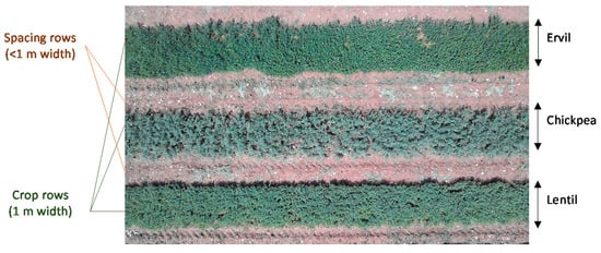
Figure 1.
Chickpea, lentil, and ervil rows. Image captured with the Parrot Bebop 2 UAV thermal camera.
The vegetative growth stage was selected as the phenologic state for image gathering. This stage was selected since, in the flowering period, the different colours of chickpea, lentil, and ervil flowers facilitate the differentiation of vegetation. Therefore, this stage presents a challenge compared with the reproductive stage. The methodology must be applied in the vegetative stage since this is the longest stage, and this is when most pests and diseases might occur and affect the reproductive stage, provoking a decrease in the yield.
2.2. Image Gathering
Images were captured by a UAV platform composed of a Parrot Bebop 2 and a FLIR ONE Pro thermal—RGB camera, see Figure 2a). The FLIR camera has a maximum visual resolution of 1440 × 1080 and HFOV/VFOV: 55 ± 1°/43 ± 1°. The use of the frontal UAV camera was discarded as overhead images from the plots are needed.
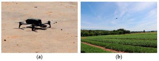
Figure 2.
Image gathering process. (a) Drone used, (b) picture of image capturing process.
The UAV was placed at 12 m and 16 m over the plots on 27 May 2021, when the plants were fully developed and starting to bloom, see Figure 2b). These heights were selected according to the positive results in [9] with images at 8 and 12 m. The selected heights and the small size of the drone ensured no draught caused by the drone’s propellers reached the leaves of the crops, which can complicate the image analysis. The plants have an approximate height of 30 to 40 cm. The day was selected to ensure good meteorological conditions and the plants’ phenological status. The camera’s exposure parameters were automatically selected, and images were acquired at 13:00 local time under clear and sunny conditions. The software of the camera automatically corrected the overexposure. For each height, at least five pictures were taken, to allow discard if any image was blurry. The three images with better quality were used. The pixel size was 0.63 cm2 and 1.1 cm2 for 12 m and 16 m, respectively.
2.3. Image Classification Process
The process followed for image classification is described as follows. First, the proccess is divided into two big blocks: the procedures for image classification, which will be conducted in the node; and the process to select the operators, thresholds, and evaluate the accuracy of the results. The second block of operations is executed as “beyond node process” to define certain parameters that will be included in the “in node process”.
The “in node process” is defined first:
- The first step is to obtain the Soil Index (SI) and the Vegetation Index (VI), defined in [18].
- After obtaining the output of both indices (SI and VI), the mathematical combination of both indices is performed to obtain the Vegetation–Soil Index (VSI). To do so, the first step is to reclassify the data of SI to generate a mask. The rule for the reclassification is the following one: if the original pixel value = 0, the newly assigned value is 0. If the original pixel value = “Else”, the newly assigned value is 1. The objective of this soil mask, or Reclassified SI (rSI), is to reduce the variability of soil pixel values in the VI to simplify the reclassification of the results after the aggregation.
- The next step is to aggregate the VSI to generate the Aggregated VSI (VSIA). The aggregation is performed to reduce the size of the picture and minimize the effect of isolated pixels, which usually represent abnormal values. For this, the operator must be selected in the “beyond node process”. The selected operator will be applied to the VSI with a cell size of 20 pixels. The cell size of 20 was set to ensure a minimum width of 8 pixels for each crop row in the images captured at 16 m.
- Once the VSIA is obtained, the soil mask (the rSI) is applied again, generating the Masked VSIA (VSIAM) to ensure that all soil pixels have a value of 0.
- The subsequent step is the reclassification in 5 classes and obtaining the Reclassified VSIAM (rVSIAM). In this step, the values used for the classification are defined according to the results of thresholds generation in the “beyond node process”.
The “beyond node process” is described below.
- The first step is to compare the best operator for aggregation of the VSI. The five operators (maximum, summation, mean, median and minimum) are compared for that purpose. The resultant aggregated VSI are compared, first visually, and then by comparing the variance of the three crop rows. In the first comparison the worthless results are excluded. Worthless results are the aggregated images in which the different crop lines cannot be identified or those with the same values. The second comparison extracts each crop row’s mean, maximum, minimum, and standard deviation (σ). After normalizing the data, each crop line’s minimum and maximum values are compared, and the operator that offers the greater variability between crops (inter-crop variability) is selected. If the operators showed similar inter-crop variability, the one with the greater intra-crop variability is selected.
- The next step is the attainment of thresholds for the VSIAM. The initial procedure is to analyze whether it is feasible to distinguish crop type. Therefore, the histograms of each crop row are obtained and mean values are compared with an ANalysis Of VAriance (ANOVA). Once ANOVA identifies whether data can be used to differentiate the crops, unsupervised classification methods are used to generate a variable number of classes. Then, the classes are merged in a supervised classification to attain the thresholds.
- Finally, the evaluation of the accuracy of rVSIAM is performed. Three areas that contain the majority of each crop row are analyzed to determine the accuracy according to the initial crop type and the classified crop type.
To summarize this information, the “in node process” and the “beyond node process” are identified in Figure 3. Blue items indicate those processes conducted in the node, while orange items display the processes conducted beyond the node. Results of beyond the node actions which are included in the node process are identified in both colours. It is important to note that the “beyond node processes” are just performed now to select the operator and the thresholds. They are not conducted in the field when the proposed approach is performed.
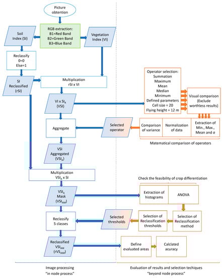
Figure 3.
Summary of followed processes presented as a flow chart.
The following mathematical procedures are applied in the node. The steps for obtaining VSI include the SI (1), the reclassification of SI (2), the VI (3), and the multiplication or reclassified SI and VI (4). The procedure for obtaining aVSI (the aggregated VSI) is included only for Summation and described in Algorithm 1 as the set of commands in Python. The same procedure is followed for other mathematical operators. The included operator in the final mathematical procedure will be defined in the results section. Finally, the multiplication for obtaining VSIAM is shown in (5). The procedure for rVSIAM (reclassified VSI aggregated and masked) is not entirely defined since the threshold for the reclassification will be defined in the Section 3. The code in Python for this procedure using letters for “a” to “e” for the thresholds for the plant species (for the class soil, = is the threshold) is presented in Algorithm 2.
| Algorithm 1: The Code for Aggregate Operation |
| # Code for Aggregate Operation import arcpy from arcpy import env from arcpy.sa import * env.workspace = “C:/sapyexamples/data” outAggreg = Aggregate(“VSI”, 20, “SUMMATION”, “TRUNCATE”, “DATA”) outAggreg.save(“C:/sapyexamples/output/VSIa” |
| Algorithm 2: The Code for Reclassify Operation |
| # Code for Reclassify Operation import arcpy from arcpy import env from arcpy.sa import * env.workspace = “C:/sapyexamples/data” outReclass1 = Reclassify(“VSIam”, “Value”, RemapRange ([[0,1], [0,a,2], [a,b,2], [b,c,3], [c,d,4], [d,e,5]])) outReclass1.save(“C:/sapyexamples/output/rVSIam”) |
3. Results
3.1. Application of Vegetation and Soil Indices
This subsection displays the raw results of applying the vegetation indices to images gathered at 16 and 12 m. In order to reduce the size of figures in this subsection, only the first picture for each flying height is shown. All images have been considered in all steps described in this subsection.
Figure 4 depicts the raw results of the initial step. Figure 4a,b show the true colour images at 16 and 12 m. Figure 4c,d present the results after applying the vegetation index at images at 16 and 12 m. Even in the raw results, it is possible to identify that different crops are characterized with different values, with higher values for ervil, followed by lentils and chickpea. The VI might take any positive integer value. A summary of values of VI for each one of the six analyzed pictures is displayed in Table 1.
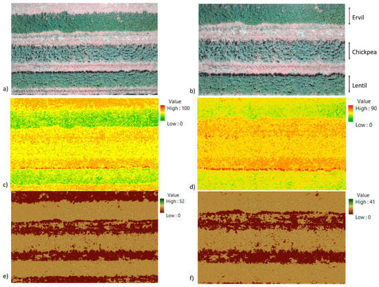
Figure 4.
Results of indices applications. (a) True colour image at 16 m; (b) true colour image at 12 m; (c) vegetation index at 16 m; (d) vegetation index at 12 m; (e) soil index at 16 m; (f) soil index at 12 m. The crops in the images from top to bottom lines are ervil, chickpea, and lentil.

Table 1.
Description of VI results for each image.
Finally, in Figure 4e,f, the raw results of the soil index are presented. In this case, in the soil index, it is possible to identify the soil with value = 0 and the vegetation, both as a crop or as weeds, in values between 1 and 52 or 41, based on whether the images are from 16 or 12 m. As for VI, SI may take any positive integer value. A summary of values of SI for each one of the six analyzed pictures is displayed in Table 2. The values for the VI and SI applied at both tested heights are similar, as shown in Table 1 and Table 2. The differences of SI or VI of images gathered at the same heights are insignificant.
Table 2.
Description of SI results for each image.
3.2. Selection of Best Aggregation Technique
This subsection describes the process followed in selecting the best aggregation technique for the proposed process. Again, and to keep a figure size that allows a good reading, the results for just the first of the three pictures gathered at 12 m of relative flying height are displayed. As in the previous subsection, all images are considered for the decisions. The input data for this step is the VSI; see Figure 5a.
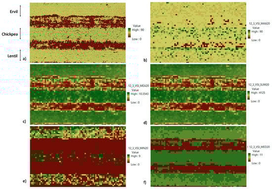
Figure 5.
Results of selection of best aggregation technique using the example of results with the first repetition at 12 m. (a) VSI; (b) aggregation technique = Maximum; (c) aggregation technique = Mean; (d) aggregation technique = Summation; (e) aggregation technique = Minimum; (f) aggregation technique = Median. The crops in the images from top to bottom lines are ervil, chickpea, and lentil.
Figure 5 displays the results of the different aggregation techniques tested in this study. In total, of five mathematical operators are included in this comparison: maximum Figure 5b, mean Figure 5c, summation Figure 5d, minimum Figure 5e, and median Figure 5f. The results show that the maximum and minimum are the worst operators for this case. Meanwhile, the results of applying the mean, median, and summation represent clearly the three crop lines. Regarding the differences in values of each crop line, the median has lower intra-crop variability and fewer differences in values in each line. Nonetheless, the values between lines, the inter-crop variability, are very low. This low inter-crop variability might preclude the differentiation of crops. On the other hand, the results of mean and summation are similar, with higher inter-crop variability than the results of the median. The summary of the VSIA for each one of the images with summation and mean operators is shown in Table 3. Considering the similar results of both aggregation operators, the analytical comparison of inter-crop and intra-crop variability is performed. The minimum and maximum values in each crop line are normalized to allow the comparison. The results of this comparison are presented in Figure 6. The minimum and maximum values are identified in blue and orange bars for each one of the crops and the aggregation operators. It is possible to determine that the variability is similar, with slightly higher variability when the mean is selected as the prefered operator.
Table 3.
Description of VSIA results for each image (including crops and soil).
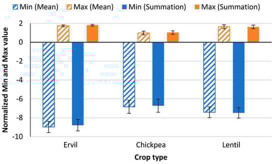
Figure 6.
Comparison of normalized mean values and standard deviation of intra-crop data variability of each crop for the summation and mean aggregation operators.
3.3. Classification of Crops
The content of this subsection is divided into two parts. In the first part, the data exploration to evaluate the possibility of differentiating the crop types is detailed. The attainment of thresholds and the evaluation of classification accuracy is presented in the second part.
3.3.1. Crop Types Differentiation
In this subsection, the classification of VSIAM by selecting a series of thresholds is displayed. At this moment, the six VSIAM (the two flying heights and the three repetitions) are used to find the most suitable thresholds.
Figure 7 depicts the six VSIAM. Figure 7a,b represent image n° 1 at flying heights of 12 and 16 m. Figure 7c,d represent images n° 2 at flying heights of 12 m and 16 m. Finally, images n° 3 at flying heights of 12 m and 16 m are depicted in Figure 7e,f. These images, the VSIAM, are used to establish the thresholds. Before analyzing the different methodologies to extract the threshold values it is necessary to evaluate if it is feasible to distinguish the crops or not. The histogram of the crop lines was calculated for the six images (three repetitions and two flying heights); see Figure 8. The histogram depicts the absolute frequency of the different pixel values for each crop type. The results indicate that differentiating between chickpea and the other two crops (ervil and lentil) is easy due to the clear differences in the values. Nonetheless, the histograms are partially superposed for crop types ervil and lentil, which complicates the classification. The average values of each crop type are obtained from the histograms. An ANOVA procedure is performed with the average values to evaluate whether it is feasible to distinguish the crop types for each of the flying heights. The results of the ANOVA, in Table 4, indicate that it is possible, in all cases, to distinguish chickpea from the rest of the crops.
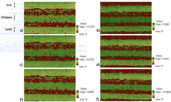
Figure 7.
VSIAM before classification of the three gathered images and the two flying heights. (a) VSIAM 12 m image n° 1, (b) VSIAM 16 m image n° 1, (c) VSIAM 12 m image n° 2, (d) VSIAM 16 m image n° 2, (e) VSIAM 12 m image n° 3, (f) VSIAM 16 m image n° 3. The crops in the images from top to bottom lines are ervil, chickpea, and lentil.
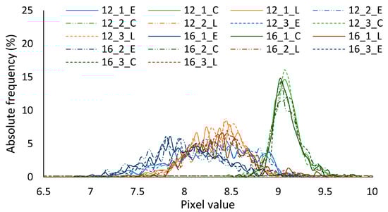
Figure 8.
Histograms for each one of the crop lines and the six studied images.
Table 4.
Summary of ANOVA results with the mean values of selected areas.
Nevertheless, it is impossible for images gathered at 12 m to distinguish between ervil and lentils. On the contrary, for images gathered at 16 m, it is feasible to determine the three crop types. The possible explanation for this phenomenon is that the complete width of the crop row of ervil and lentil is not fully included in images obtained at 12 m. Therefore, the images gathered at 12 m are not used in the next subsection.
3.3.2. Crop Types Classification
In this subsection, the crop classification is presented. First of all, the process followed to attain the threshold values is described. Then, the classified images, rVSIAM, are displayed. Finally, the accuracy of the classification for each one of the crop types is calculated based on rVSIAM.
In order to establish the thresholds for the classification of crop types, several unsupervised methods have been tested. The best results have been obtained with the unsupervised classification of data in 20 groups based on the natural breaks (Jenks). Then, those 20 groups are joined in supervised classification, creating a total of five groups (soil, ervil, lentil, chickpea, shadows). The established thresholds used to reclassify the image are shown in Table 5. The results of applying these thresholds in the reclassification to generate the rVSIAM can be seen in Figure 9a for image n° 1, Figure 9b for image n° 2, and Figure 9c for image n° 3.
Table 5.
Used thresholds for reclassification of VSIAM into new classes.
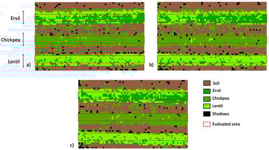
Figure 9.
rVSIAM of the three gathered images at 16 m and the identification of the studied zones to calculate the accuracy of the proposed method. (a) rVSIAM image n° 1, (b) rVSIAM image n° 2, (c) rVSIAM image n° 3. The crops in the images from top to bottom lines are ervil, chickpea, and lentil.
Three areas are selected from each image representing the three crop lines. Each area is composed of 360 pixels. These areas are used to calculate the accuracy of the proposed method. The confusion matrix that summarises the three images’ results is depicted in Table 6. The classification of chickpea is the one with higher accuracy (95% of pixels were correctly classified), followed by lentil (86%) and ervil (60%).
Table 6.
Confusion matrix of the three studied zones for the three rVSIAM using the threshold values as a classification option.
Finally, to prove that this classification option is feasible and offer accurate results, we will compare the data with a confusion matrix obtained by using Random Trees (RT). We have set 50 as the maximum number of trees and 30 as the maximum tree depth. The confusion matrix is shown in Table 7. It is possible to see that no great variation on the classification of chickpea is attained with RT. The correct classification of ervil increases from 60% to 67% by using RT. Meanwhile, the percentage decreases from 86% to 77% for lentils. Therefore, we can conclude that the accuracy of the proposed method is similar to machine learning options.
Table 7.
Confusion matrix of the three studied zones for the three rVSIAM using the threshold values and RT as classification options.
4. Discussion
The discussion is subdivided into three subsections. First, the obtained results are compared with literature to evaluate if the proposed method presents novelty compared with existing methods. Subsequently, the relevance of the proposed method for intercropping systems and the GO TecnoGAR project is analyzed. Finally, the limitations of the proposed methodology are identified.
4.1. Comparison of Results with Literature
As established in the introduction, very few papers include intercropping in their studies. Therefore, only a limited comparison of results with similar proposals can be achieved.
Before considering the details, the different mentions of intercropping in remote sensing literature are summarised. Q. Ma et al. [19] compiled information on several papers mentioning that crop identification in intercropping of multiple crops makes it difficult to attain high accuracy and that most studies focus on three to five different crops. They also mention that, although spectral and texture features calculated with UAV multispectral remote sensing data combined with an object-oriented Support Vector Machine (SVM) obtain high accuracies in mono-crop systems (up to 94% in maize [20]), there is significant interferences in mixed crop and intercropping. The authors of [19] indicate that OBject-oriented Image Analysis (OBIA) is the primary processing unit in crop identification in intercropping. However, the papers analyzed by Q. Ma et al. [19] to reach this conclusion do not analyze intercropping plots. The surveyed papers [21,22,23,24] are mainly based on heterogeneous areas with several plots. Each plot is composed of mono-crop agriculture, but the crop of each plot might be different, creating a mosaic of different plots. Although this might present a challenging task, intercropping, as it is understood in this paper, consists of the spatial alternation of two or more crops in a single plot forming rows.
The examples of remote sensing use in real intercropping systems are discussed in this paragraph. In [25], S. Huang et al. include intercropping plots in their study to evaluate the performance of their approach. They were identifying the crop type in five areas composed of a heterogeneous mosaic of mono-crop with some intercropping plots. Their methods classified the entire plot as intercropping (sunflower + zucchini), sunflower, zucchini, or corn. The accuracies of semantic segmentation ranged from 92 to 99%. R. Chew et al. [14] obtained crop classification accuracies of 96% (banana and maize) as mono-crop compared to 49% for legumes mostly cultivated under intercropped conditions. Another example can be found in [26], where M. Hegarty-Craver et al. included mono-crop and intercropping plots. Their results indicate that the intercropped plots (maize + cassava or maize + beans) are wrongly classified as another crop type (such as cassava or beans). The archived accuracies range from 67 to 91 %. Although some of these proposals might have good performance, the identification of individual crop rows is not performed in the intercropping plots. The sole example in which crop species growing in intercropping are identified is presented by M. A. Latif in [15]. In their study, 17 different crops were grown in a row intercropping plot. Images were gathered with a Phantom-4 DJI every 15 days over four months to generate a time-series analysis. The rows had a width of 1 m with spacing rows of 1 m between species. An accuracy of 99% in the identification of each crop was attained. A summary of the accuracies of the abovementioned authors is presented in Table 8.
It is possible to affirm that the proposed method attains accuracies in chickpea (95%) and lentil (86) identification aligned with the average classification of other proposals [15,24,25,26] for mono-crops in a heterogeneous mosaic with or without isolated intercropping. The accuracy for ervil classification, even though it is lower than the average classification accuracies, it is still within the range of the minimum classification accuracies of existing solutions. The obtained accuracies in intercropping areas [14] are higher than the obtained in this paper. Nonetheless, the methodology proposed in [14] is characterized by a higher complexity than the one proposed in this paper. The simplification of processes, especially avoiding time-series analysis, outweighs the decrease in the classification accuracy.
Table 8.
Summary of accuracies attained by other methods and the proposed method.
Table 8.
Summary of accuracies attained by other methods and the proposed method.
| Management | Crop/s | Source | Approach | Accuracy | Ref | ||
|---|---|---|---|---|---|---|---|
| Global | Min. | Max. | |||||
| Mono-crop in heterogeneous mosaic | Alfalta, Almond, Walnut, Vineyards, Corn, Rice, Safflower, Sunflower, Tomato, Meadow, Oat, Rye, and Wheat | ASTER satellite (3 sampling periods) | OBIA | 80 | 69 | 100 | [21] |
| Mono-crop in heterogeneous mosaic | Winter cereal stubble, Vineyards, Olive orchards, and Spring-sown sunflowers | QuickBird | OBIA | - | 16 | 100 | [22] |
| Mono-crop in heterogeneous mosaic | Rice, Greenhouse, Corn, Tree, Unripe wheat, Ripe wheat, Grassland, and Soybean | UAV (RGB camera) + DSM data | SVM | 72.94 * 94.5 ** | - | - | [23] |
| Mono-crop in heterogeneous mosaic | Grassland, Ginsen, Vinly house, Barren Paddy, Radish, and Chinese cabbage | UAV (RGB camera) | OBIA | 85 | 68 | 100 | [24] |
| Heterogeneous mosaic with mono-crop and intercrop (legumes) | Banana, Legumes, and Maize | UAV (RGB camera) | DNN | 86 | 49 | 96 | [14] |
| Mono-crop in heterogeneous mosaic with isolated intercropping | Maize, Beans, Cassava, Bananas, and Intercropped Maize | UAV (RGB camera) | Object contextual representations network | 67 | 91 | [26] | |
| Mono-crop in heterogeneous mosaic with isolated intercropping | Zucchini, Sunflower, Corn, Zucchni+Sunflower | UAV (RGB camera) | Object recognition | 92 | 99 | [25] | |
| Intercropping | Wheat, Barley, Oat, Clover, Alfalfa; Rapeseed, Mustard, Linseed, Kusumbra, Hallon, Methre, Lentil, Chickpea, Fennel, Soo ye, and Black cumin | UAV multispectral camera (8 sampling periods) | Time-series, principal components, and decision tree | 99 | [15] | ||
| Intercropping | Ervil, Chickpea, Lentil | UAV (RGB camera) | Vegetation indices, | 80 | 60 | 95 | - |
* Accuracy for RGB data. ** Accuracy for complex combined sources.
It should also be noted that only two of the reviewed papers include legumes. The first mentions lentils as lentils in intercropping [14], but does not identify the species’ canopy. On the other hand, [15] includes lentils and chickpea among their tested species. Nonetheless, no single study includes ervil as one of the evaluated species.
4.2. Relevance of Proposed Method for Intercropping Systems and Go TecnoGAR Project
Intercropping is a practice used mainly when farmers have limited access to agricultural chemicals and equipment, and is prevalent in the developed world, instead of being used as a sustainable way of cultivation [27]. For example, in Africa, corn (Zea mays L.), sorghum (Sorghum bicolor (L.) Moench), or millet (Panicum and Pennisetum spp.) are grown together with pumpkin (Cucurbita spp.), cowpeas (Vigna unguiculata (L.) Walp), pigeon peas (Cajanus cajan (L.) Millsp.), or beans (Phaseolus spp.). Cocoa (Theobroma cacao L.) grows with yams (Dioscorea spp.) or cassava (Manihot esculenta Crantz). In the tropical Americas, maize (corn) grows with beans and squash (Cucurbita spp.). In both Africa and Latin America, beans or peas (Pisum sativum L.) climb tall cornstalks while pumpkins or squash cover the ground below. This leads to less risky agriculture since the others crops can remain healthy if one crop fails.
On the other hand, agriculture in developed countries relies on mechanization and monocultures. This type of land management is subject to several problems that intercropping can alleviate, such as: (1) reduction in insect pest populations; and (2) reduced herbivore colonization, giving intercropping huge potential as an economic and ecological alternative fully compatible with modern agriculture to improve it [28,29]. When carefully designed, intercropping systems present many advantages, such as increased forage yield, enhanced weed control, reduced soil erosion and, in the case of legumes, improved soil fertility due to their symbiosis with nitrogen-fixating bacteria [30].
Nevertheless, it is important to study the behaviour of the intercropped crops since there may exist competition between species. The best way to find an optimal intercrop combination is to experiment with a number of experimental treatments for a mono-crop and mixture in competition experiments. There are a lot of studies currently being conducted to understand the mechanism of competition by examining which species or genotypes show competitive benefit when grown in mixtures or by separate [31].
When growing large extensions of intercropped similar crops (legumes, cereals, etc.), it may be difficult to assess whether one is having trouble growing or developing. UAVs provide an excellent low-cost platform to gather RGB images on demand with enough resolution to classify the crops in a plot [9,32,33,34]. As depicted in Table 6, our method presents high accuracy in chickpea classification in a lentil–ervil–chickpea intercrop test plot. Thus, the proposed methodology leads to a fast, cheap, and reliable way of estimating the canopy of each species.
In addition, the proposed methodology can be integrated with further analysis in which plant vigour is analyzed in detail for each species. It must be noted that different crops might have different phenologic states characterized by different NDVI values. Moreover, the crops can have different basal NDVI values [35,36,37]. These basal differences can cause misclassifications of the crop with regular vigour as a crop with low vigour leading to unneeded treatment.
In this context, the GO TecnoGAR project (Innovation Operational Group for the combined use of sensors and remote sensing, a holistic solution for monitoring and improving chickpea cultivation) aims to enhance the cultivation of chickpea in Spain (in the community of Madrid) and transform it through the implementation and adaptation of new technologies in agriculture. Chickpea is a legume with a high nutritional value that currently has a relatively low production in Spain. Consequently, by overcoming the technological gap, valuing improved varieties and including elements from different stages of cultivation and commercialization, GO TecnoGAR intends to improve the efficiency of the national chickpea in the agro-food industry. Overall, the proposed method will allow evaluating and comparing the individual canopy extensions for chickpeas.
4.3. Limitations of the Proposed Method
The proposed methodology, with the established operators and thresholds, is tailored for the studied scenario. This is the primary limitation, which precludes the option of using the method in intercropping systems composed of other species. Nonetheless, with the appropriate “beyond node processes”, establishing the threshold for other species might be suitable. Therefore, the proposed methodology can be extrapolated to other intercropping systems after establishing the appropriate thresholds. It is important to note that the VI used is generated to maximize the difference between a chickpea and other legumes, and it might serve for intercropping of chickpea and other species. For intercropping systems composed of completely different species, VI might be evaluated and modified if necessary. Although this limitation, it must be noted that solutions based on vegetation indices are usually tailored for specific crops and cannot be used in other crops. Most of the mentioned works in the aforementioned subsections and those included in Table 8 are tailored solutions for certain crop combinations [14,15,21,22,23,24,25,26].
Regarding the tested flying heights, although pictures are only gathered at 12 and 16 m, using aggregated results shows that images gathered at higher flying heights should be feasible. In the case of large plots that cannot be covered in a single picture, overlapping must be considered according to the recommendations of the software for flight planning. For images gathered at higher flying heights, inferior cell sizes for the operator should be selected. To establish a maximum flying height, as long as the crop row is represented by a width of 8 pixels or more in the original picture, the proposed method can be applied. There is no information about the expected results when crop rows have inferior widths.
5. Conclusions
In this paper, a methodology for identifying crop species in intercropping systems based on rows is proposed. The method has been designed to be applied by the node that gathers the images, allowing automatic recognition of crop species. The objective of this method is to provide a fast and simple option that allows further individual analyses of each crop.
The attained classification accuracy is in the range shown in similar papers that considered mono-crops in a heterogeneous mosaic, in some cases with small intercropped plots, equivalent to intercropping scenarios [14,21,22,23,24,25,26]. The sole proposal that considers and details the dimensions of intercropping in rows [15] has a higher accuracy based on time series analyses, a complex method.
In future work, the thresholds for differentiation varieties of the same species, particularly chickpea species, will be determined. The inclusion of multispectral cameras will be considered for this step and derived products such as edge detection of the gathering of data at multiple scales. The inclusion of machine learning methods, such as machine learning and SVM [38,39,40], will be explored in the future.
Author Contributions
Conceptualization, L.P. and D.M.-C.; methodology, L.P.; software, L.P. and D.M.-C.; validation, P.V.M., J.F.M. and J.L.; formal analysis, L.P.; data curation, L.P.; writing—original draft preparation, L.P. and D.M.-C.; writing—review and editing, L.P.; supervision, P.V.M., J.F.M. and J.L.; project administration, P.V.M.; funding acquisition, P.V.M., J.F.M. and J.L. All authors have read and agreed to the published version of the manuscript.
Funding
This research was partially funded by the “Programa Estatal de I+D+i Orientada a los Retos de la Sociedad, en el marco del Plan Estatal de Investigación Científica y Técnica y de Innovación 2017–2020” (Project code: PID2020-114467RR-C31 and PID2020-114467RR-C33), and by “Proyectos de innovación de interés general por grupos operativos de la Asociación Europea para la Innovación en materia de productividad y sostenibilidad agrícolas (AEI-Agri)” in the framework “Programa Nacional de Desarrollo Rural 2014–2020”, GO TECNOGAR, and by Conselleria de Educación, Cultura y Deporte, through “Subvenciones para la contratación de personal investigador en fase postdoctoral” APOSTD/2019/04.
Data Availability Statement
The data presented in this study are available on request from the corresponding author. The data are not publicly available due to privacy constraints.
Acknowledgments
This work has been conducted based on images gathered in the facilities of AGROSA SEMILLAS SELECTAS S.A.
Conflicts of Interest
The authors declare no conflict of interest.
References
- Kopittke, P.M.; Menzies, N.W.; Wang, P.; McKenna, B.A.; Lombi, E. Soil and the intensification of agriculture for global food security. Environ. Int. 2019, 132, 105078. [Google Scholar] [CrossRef] [PubMed]
- Foster, S.; Pulido-Bosch, A.; Vallejos, Á.; Molina, L.; Llop, A.; MacDonald, A.M. Impact of irrigated agriculture on groundwater-recharge salinity: A major sustainability concern in semi-arid regions. Hydrogeol. J. 2018, 26, 2781–2791. [Google Scholar] [CrossRef] [Green Version]
- Zeraatpisheh, M.; Bakhshandeh, E.; Hosseini, M.; Alavi, S.M. Assessing the effects of deforestation and intensive agriculture on the soil quality through digital soil mapping. Geoderma 2020, 363, 114139. [Google Scholar] [CrossRef]
- Layek, J.; Das, A.; Mitran, T.; Nath, C.; Meena, R.S.; Yadav, G.S.; Shivakumar, B.G.; Kumar, S.; Lal, R. Cereal+ legume intercropping: An option for improving productivity and sustaining soil health. In Legumes for Soil Health and Sustainable Management; Springer: Singapore, 2018; pp. 347–386. [Google Scholar]
- Van Oort, P.A.J.; Gou, F.; Stomph, T.J.; van der Werf, W. Effects of strip width on yields in relay-strip intercropping: A simulation study. Eur. J. Agron. 2020, 112, 125936. [Google Scholar] [CrossRef]
- Parra, L.; Torices, V.; Marín, J.; Mauri, P.V.; Lloret, J. The use of image processing techniques for detection of weed in lawns. In Proceedings of the Fourteenth International Conference on Systems (ICONS 2019), Valencia, Spain, 24–28 March 2019; pp. 24–28. [Google Scholar]
- Parra, L.; Marin, J.; Yousfi, S.; Rincón, G.; Mauri, P.V.; Lloret, J. Edge detection for weed recognition in lawns. Comput. Electron. Agric. 2020, 176, 105684. [Google Scholar] [CrossRef]
- Osorio, K.; Puerto, A.; Pedraza, C.; Jamaica, D.; Rodríguez, L. A deep learning approach for weed detection in lettuce crops using multispectral images. AgriEngineering 2020, 2, 471–488. [Google Scholar] [CrossRef]
- Parra, L.; Mostaza-Colado, D.; Yousfi, S.; Marin, J.F.; Mauri, P.V.; Lloret, J. Drone RGB Images as a Reliable Information Source to Determine Legumes Establishment Success. Drones 2021, 5, 79. [Google Scholar] [CrossRef]
- Bégué, A.; Arvor, D.; Bellon, B.; Betbeder, J.; De Abelleyra, D.; Ferraz, R.P.D.; Lebourgeois, V.; Lelong, C.; Simões, M.; Verón, S.R. Remote sensing and cropping practices: A review. Remote Sens. 2018, 10, 99. [Google Scholar] [CrossRef] [Green Version]
- Jin, Z.; Azzari, G.; Burke, M.; Aston, S.; Lobell, D.B. Mapping smallholder yield heterogeneity at multiple scales in Eastern Africa. Remote Sens. 2017, 9, 931. [Google Scholar] [CrossRef] [Green Version]
- Liu, C.; Zhang, Q.; Tao, S.; Qi, J.; Ding, M.; Guan, Q.; Wu, B.; Zhang, M.; Nabil, M.; Tian, F.; et al. A new framework to map fine resolution cropping intensity across the globe: Algorithm, validation, and implication. Remote Sens. Environ. 2020, 251, 112095. [Google Scholar] [CrossRef]
- Li, Z.; Fox, J.M. Mapping rubber tree growth in mainland Southeast Asia using time-series MODIS 250 m NDVI and statistical data. Appl. Geogr. 2012, 32, 420–432. [Google Scholar] [CrossRef]
- Chew, R.; Rineer, J.; Beach, R.; O’Neil, M.; Ujeneza, N.; Lapidus, D.; Miano, T.; Hegarty-Craver, M.; Polly, J.; Temple, D.S. Deep Neural Networks and Transfer Learning for Food Crop Identification in UAV Images. Drones 2020, 4, 7. [Google Scholar] [CrossRef] [Green Version]
- Latif, M.A. Multi-crop recognition using UAV-based high-resolution NDVI time-series. J. Unmanned Veh. Syst. 2019, 7, 207–218. [Google Scholar] [CrossRef]
- Diebel, J.; Norda, J.; Kretchmer, O. The Weather Year Round Anywhere on Earth; Weather Spark: Hennepin County, MN, USA, 2018. [Google Scholar]
- Singh, F.; Diwakar, B. Chickpea Botany and Production Practices. 1995. Available online: http://oar.icrisat.org/2425/1/Chickpea-Botany-Production-Practices.pdf (accessed on 5 February 2022).
- Parra, L.; Yousfi, S.; Mostaza, D.; Marín, J.F.; Mauri, P.V. Propuesta y comparación de índices para la detección de malas hierbas en cultivos de garbanzo. In Proceedings of the XI Congreso Ibérico de Agroingeniería 2021, Valladolid, Spain, 11 November 2021. [Google Scholar]
- Ma, Q.; Han, W.; Huang, S.; Dong, S.; Li, G.; Chen, H. Distinguishing Planting Structures of Different Complexity from UAV Multispectral Images. Sensors 2021, 21, 1994. [Google Scholar] [CrossRef] [PubMed]
- Hall, O.; Dahlin, S.; Marstorp, H.; Archila Bustos, M.F.; Öborn, I.; Jirström, M. Classification of maize in complex smallholder farming systems using UAV imagery. Drones 2018, 2, 22. [Google Scholar] [CrossRef] [Green Version]
- Peña-Barragán, J.M.; Ngugi, M.K.; Plant, R.E.; Six, J. Object-based crop identification using multiple vegetation indices, textural features and crop phenology. Remote Sens. Environ. 2011, 115, 1301–1316. [Google Scholar] [CrossRef]
- Castillejo-González, I.L.; López-Granados, F.; García-Ferrer, A.; Peña-Barragán, J.M.; Jurado-Expósito, M.; de la Orden, M.S.; González-Audicana, M. Object-and pixel-based analysis for mapping crops and their agro-environmental associated measures using QuickBird imagery. Comput. Electron. Agric. 2009, 68, 207–215. [Google Scholar] [CrossRef]
- Liu, B.; Shi, Y.; Duan, Y.; Wu, W. UAV-based Crops Classification with joint features from Orthoimage and DSM data. International Archives of the Photogrammetry. Remote Sens. Spat. Inf. Sci. 2018, 42, 1023–1028. [Google Scholar]
- Park, J.K.; Park, J.H. Crops classification using imagery of unmanned aerial vehicle (UAV). J. Korean Soc. Agric. Eng. 2015, 57, 91–97. [Google Scholar]
- Huang, S.; Han, W.; Chen, H.; Li, G.; Tang, J. Recognizing Zucchinis Intercropped with Sunflowers in UAV Visible Images Using an Improved Method Based on OCRNet. Remote Sens. 2021, 13, 2706. [Google Scholar] [CrossRef]
- Hegarty-Craver, M.; Polly, J.; O’Neil, M.; Ujeneza, N.; Rineer, J.; Beach, R.H.; Lapidus, D.; Temple, D.S. Remote crop mapping at scale: Using satellite imagery and UAV-acquired data as ground truth. Remote Sens. 2020, 12, 1984. [Google Scholar] [CrossRef]
- Machado, S. Does intercropping have a role in modern agriculture? J. Soil Water Conserv. 2009, 64, 55A–57A. [Google Scholar] [CrossRef] [Green Version]
- Horwith, B. A Role for Intercropping in Modern Agriculture. BioScience 1985, 35, 286–291. [Google Scholar] [CrossRef] [Green Version]
- Risch, S.J. Intercropping as cultural pest control: Prospects and limitations. Environ. Manag. 1983, 7, 9–14. [Google Scholar] [CrossRef]
- Ćupina, B.; Mikić, A.; Stoddard, F.L.; Krstić, Đ.; Justes, E.; Bedoussac, L.; Fustec, J.; Pejić, B. Mutual Legume Intercropping for Forage Production in Temperate Regions. In Genetics, Biofuels and Local Farming Systems; Sustainable Agriculture Reviews; Lichtfouse, E., Ed.; Springer: Dordrecht, The Netherlands, 2011; Volume 7. [Google Scholar] [CrossRef]
- Mead, R.; Riley, J. A Review of Statistical Ideas Relevant to Intercropping Research. J. R. Stat. Soc. Ser. A Gen. 1981, 144, 462–487. [Google Scholar] [CrossRef]
- Arcidiacono, C.; Porto, S.M.C. Classification of Crop-Shelter Coverage by Rgb Aerial Images: A Compendium of Experiences and Findings. J. Agric. Eng. 2010, 41, 1–11. [Google Scholar] [CrossRef]
- Fawakherji, M.; Youssef, A.; Bloisi, D.; Pretto, A.; Nardi, D. Crop and Weeds Classification for Precision Agriculture Using Context-Independent Pixel-Wise Segmentation. In Proceedings of the Third IEEE International Conference on Robotic Computing (IRC), Naples, Italy, 25–27 February 2019; pp. 146–152. [Google Scholar] [CrossRef]
- Su, J.; Coombes, M.; Liu, C.; Zhu, Y.; Song, X.; Fang, S.; Chen, W.H. Machine learning-based crop drought mapping system by UAV remote sensing RGB imagery. Unmanned Syst. 2020, 8, 71–83. [Google Scholar] [CrossRef]
- Liu, P.; Chen, X. Intercropping classification from GF-1 and GF-2 satellite imagery using a rotation forest based on an SVM. ISPRS Int. J. Geo-Inf. 2019, 8, 86. [Google Scholar] [CrossRef] [Green Version]
- Abaye, A.O.; Trail, P.; Thomason, W.E.; Thompson, T.L.; Gueye, F.; Diedhiou, I.; Diatta, M.B.; Faye, A. Evaluating Intercropping (Living Cover) and Mulching (Desiccated Cover) Practices for Increasing Millet Yields in Senegal. 2016. Available online: https://pdfs.semanticscholar.org/e11b/debf02cf1d6471c9bef5b9ffea0c17519ec1.pdf?_ga=2.49841638.1325397891.1644977379-1028145369.1629703351 (accessed on 5 February 2022).
- Bogie, N.A.; Bayala, R.; Diedhiou, I.; Dick, R.P.; Ghezzehei, T.A. Intercropping with two native woody shrubs improves water status and development of interplanted groundnut and pearl millet in the Sahel. Plant Soil 2019, 435, 143–159. [Google Scholar] [CrossRef]
- Guo, Y.; Fu, Y.; Hao, F.; Zhang, X.; Wu, W.; Jin, X.; Bryant, C.R.; Senthilnath, J. Integrated phenology and climate in rice yields prediction using machine learning methods. Ecol. Indic. 2021, 120, 106935. [Google Scholar] [CrossRef]
- Chang, C.C.; Lin, C.J. LIBSVM: A library for support vector machines. ACM Trans. Intell. Syst. Technol. TIST 2011, 2, 1–27. [Google Scholar] [CrossRef]
- Joachims, T. Making Large-Scale SVM Learning Practical (No. 1998, 28); Technical Report; Universität Dortmund: Dortmund, Germany, 1998. [Google Scholar]
Publisher’s Note: MDPI stays neutral with regard to jurisdictional claims in published maps and institutional affiliations. |
© 2022 by the authors. Licensee MDPI, Basel, Switzerland. This article is an open access article distributed under the terms and conditions of the Creative Commons Attribution (CC BY) license (https://creativecommons.org/licenses/by/4.0/).