Article

A Multisensor Fusion-Based Cooperative Localization Scheme in Vehicle Networks

1
National Time Service Center, Chinese Academy of Sciences, Xi’an 710600, China
2
School of Electronic, Electronial and Communication Engineering, University of Chinese Academic of Sciences, Beijing 100049, China
3
School of Astronomy and Space Science, University of Chinese Academic of Sciences, Beijing 100049, China
4
School of Telecommunications Engineering, Xidian University, Xi’an 710000, China
*
Author to whom correspondence should be addressed.
Electronics 2022, 11(4), 603; https://doi.org/10.3390/electronics11040603
Submission received: 3 January 2022 / Revised: 8 February 2022 / Accepted: 14 February 2022 / Published: 16 February 2022
(This article belongs to the Collection Advance Technologies of Navigation for Intelligent Vehicles)

Abstract

:
Utilizing the measured distance and information exchanged between two different nodes to cooperatively locate in a mobile network has become a solution to replace global navigation satellite system (GNSS) positioning. However, the localization accuracy of the belief propagation-based cooperative localization scheme is substantially influenced by the number of neighbors. In this paper, we propose a cooperative localization scheme combined with a trajectory tracking algorithm. With an insufficient number of neighbors, the trajectory tracking algorithm is utilized to participate in the positioning process of agents. Concretely, we carry out sensor information fusion and utilize quantum-behaved, particle-swarm-optimized, bidirectional long short-term memory (QPSO–BiLSTM) as a trajectory tracking strategy, to precisely predict the positions of agents. It is evident from simulations and results that the proposed cooperative localization scheme performs better than the belief propagation (BP)-based cooperative localization scheme in position error.

1. Introduction

With an increase in intelligent transportation system (ITS) applications, there is an imperative demand for precise positioning information [1]. The issue of vehicle positioning for vehicle networks has received a substantial amount of critical attention. Generally, global navigation satellite-based system (GNSS) provides accurate location information. However, due to coverage and signal strength limitations, the GNSS is not suited for all vehicles in ITS applications. Therefore, various localization approaches have been proposed to overcome this limitation. Cellular localization relies on distance measurements, in which the user’s position is calculated on the base stations. Similarly, localization schemes based on ultrawideband (UWB) and Wi-Fi obtain accurate position information, whose accuracy ranges from 1 m to 10 m. In addition, radio-based positioning techniques with novel 5G technologies stimulate the development of high-precision localization, where millimeter wave (mmWave), multiple-input–multiple-output (MIMO), and direct device-to-device (D2D) communication is beneficial to obtain submeter localization accuracy [2].
Amidst dissimilar localization schemes and the development of 5G technologies, cooperative localization has emerged as an interesting candidate. The low power large bandwidth ultrawideband (UWB) communication is beneficial for acquiring accurate measurements [3,4]. Specifically, the distance between two different nodes is measured via the time of arrival (TOA) [5], time difference of arrival (TDOA) [6], and received signal strength indication (RSSI) [7] in mmWave frequencies. In addition, a larger number of antennas accurately estimate the angle of arrival (AOA) [8]. The cooperative localization scheme performs location estimation in utilizing information exchanged between two nodes after the ranging information is obtained. However, the network size, anchor node distribution, and neighbor selection greatly impact the location accuracy.
Currently, the cooperative localization scheme, which is composed of a centralized-based method and distributed-based method, has shown significant achievements among localization systems [9]. The centralized-based approach has been implemented using a central processor to obtain measurements for agents’ positions [10], whereas the agents estimate positions via measurements of neighboring nodes in the distributed-based approach. In addition, the Bayesian-based cooperative localization scheme is employed due to its excellent performance. Ihler et al. proposed a nonparametric belief propagation (NBP) algorithm to minimize the number of communication nodes [11]. Wymeersch et al. [12] proposed a classical localization scheme based on the sum-product algorithm over a wireless network referred to as the belief propagation (BP) algorithm, which is robust to various scenarios but still has a large communication overhead. The variational message-passing algorithm was carried out by Pedersen et al., to solve the above problem, as well as to improve the positioning accuracy [13]. However, the above methods are not suited for mobile users.
Therefore, the trajectory tracking method is combined with a cooperative localization scheme and applied in mobile networks. Garcia-Fernandez et al. [14] implemented the Kalman filter to update the position of the Gaussian distribution and proposed a posterior linearization belief propagation (PLBP) algorithm to address the nonlinear range measurement. Cakmak et al. [15] proposed a distributed belief propagation algorithm combined with tracking mobile agents and obtained the position. Hehdly et al. [16] utilized Kalman and particle filters as distributed tracking filters, to perform cooperative localization. The particle filter is associated with the BP model and further reduces the position error for dynamic networks [17,18,19]. Although the above methods are well utilized in mobile networks, additional research on vehicular networks has been carried out. Eom et al. [20] developed a deep-learning-based cooperative localization technique for high localization accuracy and real-time operation in vehicle networks. Similarly, Kim et al. [21] employed multimodel probability and hypothetical density filters, to address multipath signals for cooperative vehicle positioning and mapping. A novel sensor tracking algorithm-based semidefinite programming (SDP) was designed by Denis et al. to mitigate non-line-of-sight (NLOS) propagation and to improve the position accuracy [22]. However, the limitation of the above methods has required enough neighbors (numbers > 3) to obtain accurate location information.
The main contributions of the paper are summarized here. We proposed a cooperative localization method that is based on the trajectory tracking strategy of vehicles, to improve the localization accuracy without a sufficient number of neighbors. Specifically, the BP algorithm is utilized to obtain vehicle localization. Subsequently, we formulate sensor information fusion to learn the location from the BP algorithm and to utilize bidirectional long short-term memory (BiLSTM) with quantum-behaved particle swarm optimization (QPSO) as a trajectory tracking strategy to precisely predict vehicles’ positions. Simulation and results demonstrate that the proposed cooperative localization scheme based on the trajectory tracking strategy performs well for vehicle networks.
The remaining part of the paper is organized as follows: In Section 2, the details of the cooperative localization scheme are analyzed. In Section 3, we develop the trajectory tracking-based cooperative localization scheme. The simulation results are given in Section 4 to verify the effectiveness of the proposed method. Concluding remarks are presented in Section 5.

2. Materials for the Cooperative Localization Scheme
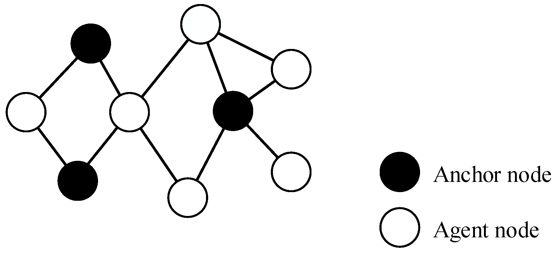
2.1. System Model

The synchronous network is composed of multiple agents and some static anchors at discrete time n = { 1 , , N } . The agents and anchors represent vehicles and roadside units (RSUs). The anchors have known and fixed locations. The agents consist of mobile nodes and static nodes without location information. Figure 1 describes the localization system with the factor graph, which consists of nodes and edges . = { a , b } is partitioned into anchors a and agents b . Similarly, indicates the communication links. Due to the limitation of the communication range with nodes, each agent only locates itself in a distributed localization system.
The state of agent node k is denoted in vector x k n , where x k n [ x k n , y k n , x ˙ k n , y ˙ k n ] T . x ˙ k n and y ˙ k n represent the speeds in the x direction and y direction, respectively, at time n . In addition, x k n , y k n represents the 2D position of agent k at time n , in the mobile network, and is given by
x k n = G x k n 1 + u k n
where u k n N ( u k n ; 0 , Σ u k ) with Σ u 2 , i = σ u 2 , i 2 F F T ; and G and F are defined here [23].
G = [ 1 0 Δ t 0 0 1 0 Δ t 0 0 1 0 0 0 0 1 ] , F = [ Δ t 2 / 2 0 0 Δ t 2 / 2 Δ t 0 0 Δ t ]
where Δ t is the duration of the one-time step. Since agents independently move, the state transition function is defined as
p ( x k n | x k n 1 ) exp ( 1 2 x k n G x k n Σ u k 1 2 )
The initial state x k 0 obeys an independent Gaussian distribution, with x k 0 N ( x k 0 ; μ f k x k 0 , Σ f k x k 0 ) , and μ f k x k 0 , Σ f k x k 0 are the mean and covariance of the initial state of the prediction message, respectively. In addition, all agents’ joint prior probability density function (PDF) in status update time n is given by
p ( x 1 : n ) = i = 1 n k p ( x k i | x k i 1 )
The noisy measurement is obtained between agent node k and node l at time n
z k , l n = x k n x l n + w k , l n
where w k , l n is the measured noise and obeys a Gaussian distribution with variance σ w 2 . In particular, the measurement provides the likelihood function p ( z k l n | x k n , x l n ) between each pair of neighboring nodes ( k , l ) , and the likelihood function is given by
p ( z k l n | x k n , x l n ) = 2 π ( σ k l n ) 2 exp { ( z k l n x k n x l n ) 2 2 ( σ k l n ) 2 }
where σ k l n is the standard deviation of the distance between node k and node l at time n . In addition, each agent k has a prior distribution p k ( x k ) . The range measurements between two nodes at different times are conditional independent, and the joint distribution is defined as
p ( x 1 , , x k | { z k , l } ) = k p ( x k ) ( k , l ) p ( z k , l | x k , x l )

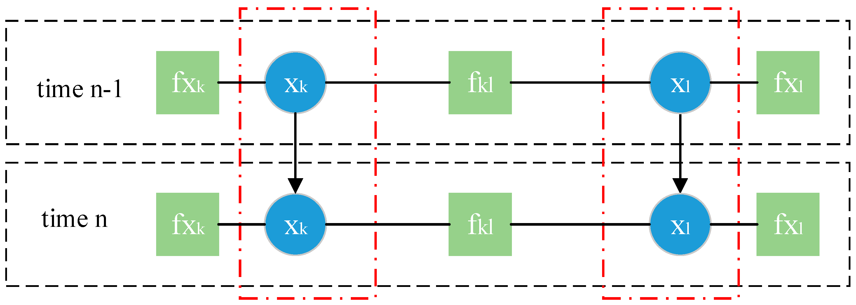
2.2. BP Algorithm for Cooperative Localization

The BP algorithm, which is based on a factor graph, obtained the position information via message passing and is a classical cooperative location scheme. The factor graph is composed of variable nodes, factor nodes, and edges that are connected to certain variable nodes with certain factor nodes.
The minimum mean-square error (MMSE) estimator is utilized to estimate state x k n from the total measurement vector z 1 : n and to obtain the position information
x ^ k n x k n p ( x k n | z 1 : n ) d x k n
where p ( x k n | z 1 : n ) is the posterior PDF obtained via the BP message passing algorithm, and z 1 : n [ z i ] i = 1 n is with z i [ z k , l i ] ( k , l ) n .
The prediction and cooperative message consist of the progress of the BP algorithm. For the measurement message, the message between agent node k and node l from the factor is sent to the variable and obtained in the inverse direction. The process is given by
μ f k l x k n ( j ) ( x k n ) = p ( z k l n | x k n , x l n ) l k μ x k n f k l ( j 1 ) ( x k n ) d x k n
μ x k n f k l ( j ) ( x k n ) = μ f k x k n l S k / l μ f k l x k n ( j ) ( x k n )
where μ x k n f k l ( j ) is the message from variable x k n to factor f k l at the j ( 1 , N i t e r ) iteration, and S k is the neighboring node set of agent k. Here, the belief is obtained
b ( j ) ( x k n ) = μ f k x k n ( x k n ) l S k μ f k l x k n ( j ) ( x k n )
which consists of prediction messages and all measured messages from neighbors. For the prediction message style, the message is defined as
μ f k x k n ( x k n ) = p ( x k n | x k n 1 ) b ( N iter ) ( x k n 1 ) d x k n 1
where Niter denotes the final number of iterations of message passing.
The BP message passing in the mobile network is revealed in Figure 2. The black boxes correspond to the transmission process of the “measurement message”, and the red boxes represent the “prediction message”. In addition, edges without arrows between two nodes are communication links, and the arrows indicate conversion within nodes.

3. Methods

In this section, we formulate a cooperative localization scheme that employs the BP message passing algorithm to locate and utilize the BiLSTM model optimized via the QPSO algorithm to obtain the position prediction while agents are located without a sufficient number of neighbors.

3.1. Position Calculation

Since the number of agent’s neighbors is less than 3 in the positioning process, the localization performance of the BP algorithm for the mobile agent obtains poor accuracy [24]. Therefore, we developed a localization scheme that combines the BP algorithm with a tracking algorithm based on data fusion for the mobile agents.
The fusion technique was employed accurately and robustly in trajectory tracking. In [25,26], an inertial navigation system (INS) and UWB fusion system using a particle filter for pedestrian tracking was proposed to compensate for the insufficient number of anchor nodes in the UWB. Alvarez-Merino et al. [27] fused the UWB and long-term evolution (LTE) with an extended Kalman filter, to solve the above problem. However, the localization scenarios restrict the accuracy of filter-based fusion localization approaches. To address the filter-based fusion localization problem, deep learning approaches were employed for fusing multiple localization techniques instead of filter-based fusion approaches. In [28], the long short-term memory (LSTM) network for data fusion in indoor localization was proposed to address extreme environments.
We employed the bidirectional LSTM network with the QPSO algorithm as the tracking algorithm to learn the motion trajectories for the mobile agents and to further improve the localization accuracy of the mobile agents. In a mobile network, agents k b perform the BP algorithm to estimate state x k n after learning the position information via the QPSO–BiLSTM model.
For the agents, we applied Equations (9)–(12) to estimate their locations. According to the likelihood Equation (12), the “prediction message” is given by
μ f k x k n ( x k n ) N ( x k n ; m x k n , Σ f k x k n )
where the mean and variance of μ f k x k n are
m x k n = G μ x k n f k
Σ f k x k n = G Σ x k n f k G T + Σ u k
The messages from factors to vertices in the ( j ) iteration is determined to be
μ f k l x k n ( j ) ( x k n ) N ( x k n ; m f k l x k n ( j ) , ( σ f k l x k n ( j ) ) 2 )
where the parameters for the location coordinates are
m f k l x k n ( j ) = z k l n ( x k n 1 x l n 1 ) x k n 1 x l n 1 + m x l n f k l ( j 1 )
( σ f k l x k n ( j ) ) 2 = ( σ x l n f k l ( j 1 ) ) 2 + σ d 2
Similarly, the message from factors to vertices is determined to be
μ x k n f k l ( j ) ( x k n ) N ( x k n ; m x k n f k l ( j ) , ( σ x k n f k l ( j ) ) 2 )
where the parameters for the location coordinates are
m x k n f k l ( j ) = m x k n ( j ) ( σ f k l x k n ( j ) ) 2 m f k l x k n ( j ) ( σ x k n ( j ) ) 2 ( σ f k l x k n ( j ) ) 2 ( σ x k n ( j ) ) 2
( σ x k n f i j ( j ) ) 2 = ( σ x k n ( j ) ) 2 ( σ f k l x k n ( j ) ) 2 ( σ f k l x k n ( j ) ) 2 ( σ x k n ( j ) ) 2 .
The agents are calculated with Equation (11) after the incoming message from neighbors is collected, and the belief is given by
b ( j ) ( x k n ) N ( x k n ; m x k n ( j ) , ( σ x k n ( j ) ) 2 )
where the mean and variance of b ( l ) ( x k n ) for iteration are defined as
m x k n ( j ) = ( σ x k n ( j ) ) 2 ( m f k x k n σ f k x k n 2 + l S k , n m f k l x k n ( j ) ( σ f k l x k n ( j ) ) 2 )
( σ x k n ( j ) ) 2 = ( ( σ f k x k n ) 2 + l S k , n ( σ f k l x k n ( j ) ) 2 ) 1
The location process obtains the location information for agents via the BP algorithm combined with our proposed tracking scheme. The details are illustrated in Algorithm 1.
Algorithm 1. Cooperative localization and tracking.
Initialization: At time 0 agent k b drawn from a prior pdf p ( x l 0 ) and anchors with accurate locations compose a cooperative network. The distances z k , l 0 among nodes are given.
For n = 1 to Time
Step 1—Prediction: For agent k b , the prediction messages are calculated to substitute the state transition pdf p ( x k n | x k n 1 ) ;
Step 2—BP message passing: The agent k b exchanges information among neighbors and calculates the likelihood function μ f k l x k n ( j ) ( x k n ) and μ x k n f k l ( j ) ( x k n ) ;
Step 3—Estimation location: The agents approximate their locations via the MMSE algorithm using the belief and incoming messages. The QPSO–BiLSTM method learns the location of the agent k b . If the number of its neighbors is less than 3, the agent k b uses the prediction of the QPSO–BiLSTM method as its location.
End for

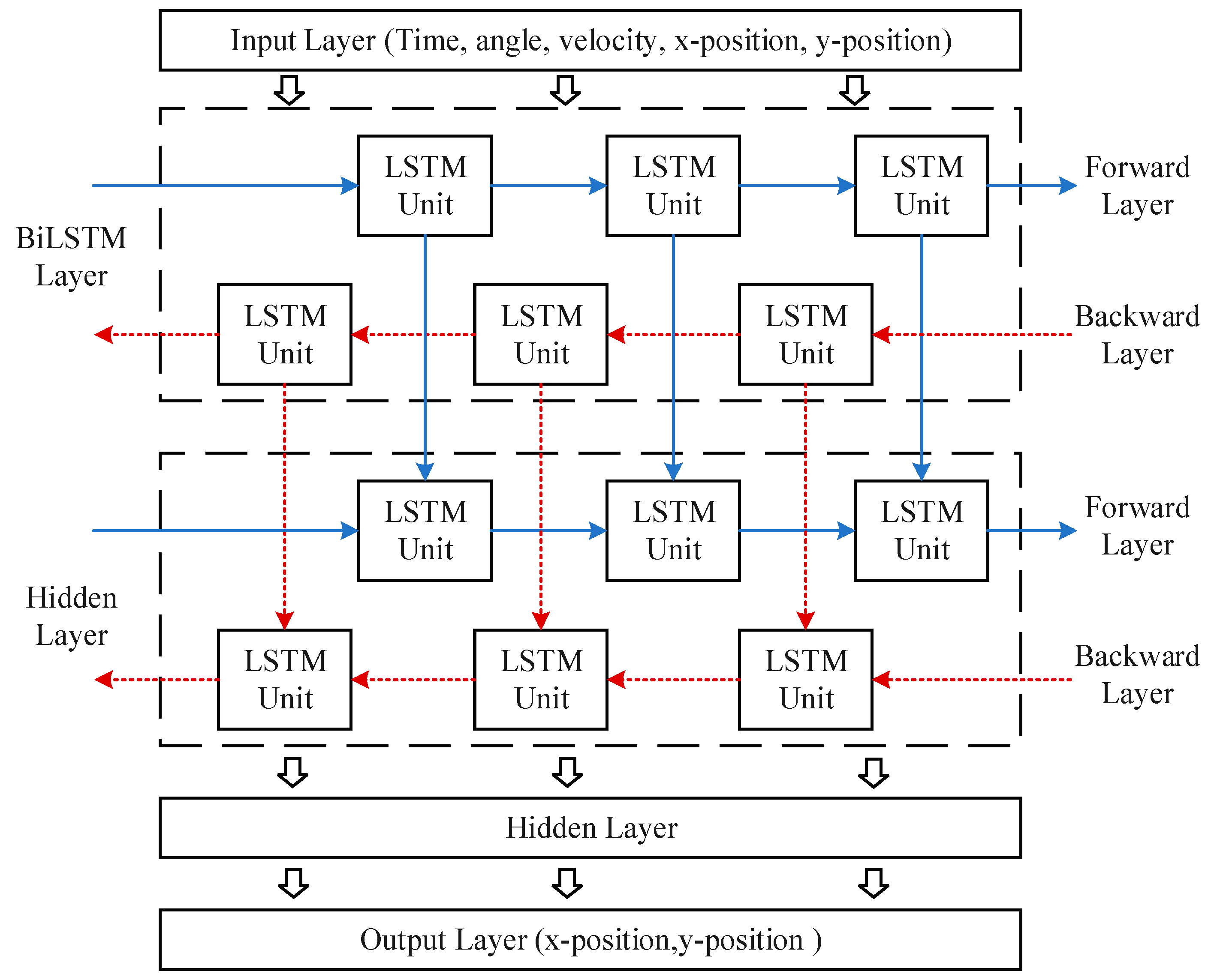
3.2. Sensor Information Fusion and Node Tracking

Information fusion is the process of combining the measured data and information originating from different sensors to produce a comprehensive model. In this process, each sensor delivers independent measurements of features. Typical information fusion models contain Joint Directors of Laboratories (JDL) and the Waterfall fusion model; a detailed explanation of the JDL architecture and process is given in [29]. In our case, the fusion of sensor information in a target node occurs at level 1 of the JDL model. The 5G information consists of the angle of the target node, position, and time. Similarly, the composition of sensor information is velocity. The deployment from different sensors is developed in Table 1.
The results of sensor data fusion are utilized to predict the location information of the target node at the next time. Among the various tracking prediction models, the class of recurrent neural networks (RNNs) has emerged as an interesting candidate. The LSTM model is a kind of classical RNN neural network. Compared with the RNN, the neuron has added input gate i, forget gate f, output gate o, and internal memory unit c. The LSTM model solves the long-term dependence problem in the RNN via the special architecture, and the output model attains optimized preference over the RNN, hidden Markov model (HMM), and Kalman filtering. However, the LSTM model preserves only information from the past, whereas the BiLSTM model preserves information from both the past and future. In addition, the BiLSTM model captures the underlying context better, bypassing the input information in the forwarding and backward directions.
The BiLSTM position prediction model was implemented using the deep learning toolboxes MATLAB version 2021a. The BiLSTM model is composed of forwarding and backward LSTM units, an input layer, a hidden layer, and an output layer; their architecture is shown in Figure 3. Each LSTM unit is derived from the RNN and has four additional portions denoted as gate i, forget gate f, output gate o, and internal memory unit c. Additionally, the hidden layer output h t , the function of the output gate (O), and the function of the memory cell (C) are given below.
h t = O t tanh ( C t )  
C t = f t C t 1 + i t tanh ( W x c p t + W h c h t 1 + b c )  
O t = σ ( W x o p t + W h o h t 1 + W c o c t + b o )
where p t is the input vector to the LSTM unit; σ and tanh are the activation functions; i t and f t are the input gate function and forget gate function, respectively; the input weight matrix and hidden weight matrix of the memory unit and output gates are represented by W x c and W h c , and W x o and W h o , respectively; b c ,   b o are bias vector parameters that need to be learned during training. In [30,31], the authors detailed the LSTM architecture and functions.
The BiLSTM architecture performs forward- and reverse-direction training processes. The input of fusion via BiLSTM layers and hidden layers holds the information and the results obtained from the output layer. Here, the Xinput component is employed in the analysis.
X i n p u t = ( T i m e , v e l o c i t y , A n g l e , X p o s i t i o n , Y p o s i t i o n )  
Y t o u t p u t s = W h y h t + W h y h t + b y  
where Y t o u t p u t s denotes the prediction results of the agent’s position, and h t , W h y and W h y , h t are the indicated weight matrix and hidden layer outputs, respectively. In addition, b y represents the bias matrix.
The results of position prediction have profound impacts on cooperative location. Therefore, we combined the QPSO algorithm to facilitate search ranges, train, and adjust the learning rate, epochs, and the number of hidden neurons, to avoid minimum local phenomenon and to reduce the error. The QPSO algorithm, which is an important improvement in the PSO algorithm, performs well with the classical PSO algorithm via the randomness of increased particle positions. The detailed explanations and application of the QPSO algorithm are given in [32,33]. Here, the specific steps in position prediction are illustrated as follows:
Step 1.
Obtain information about the sensor and preprocess it;
Step 2.
Obtain the training data and initialize the parameters;
Step 3.
Randomly initialize and input parameters into the network and utilize the MSE function as the fitness function to train and achieve the fitness value;
Step 4.
Update the location and velocity of the parameters;
Step 5.
Repeat steps 3–4 until the termination criterion is satisfied;
Step 6.
Output the optimal weights as the initial weights of the neural network and train the network to obtain the coordinate value.

4. Results

In this section, we present the simulation results of the proposed localization scheme and further analyze the impact of the tracking algorithm on the proposed scheme.

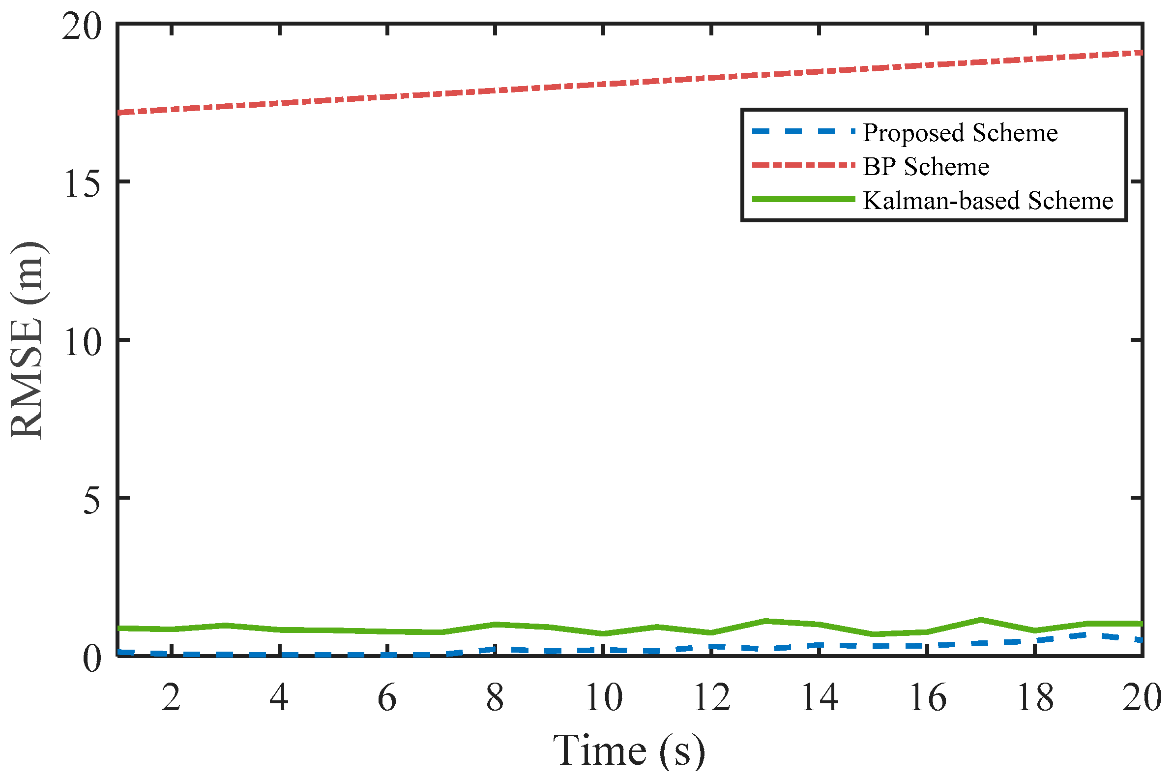
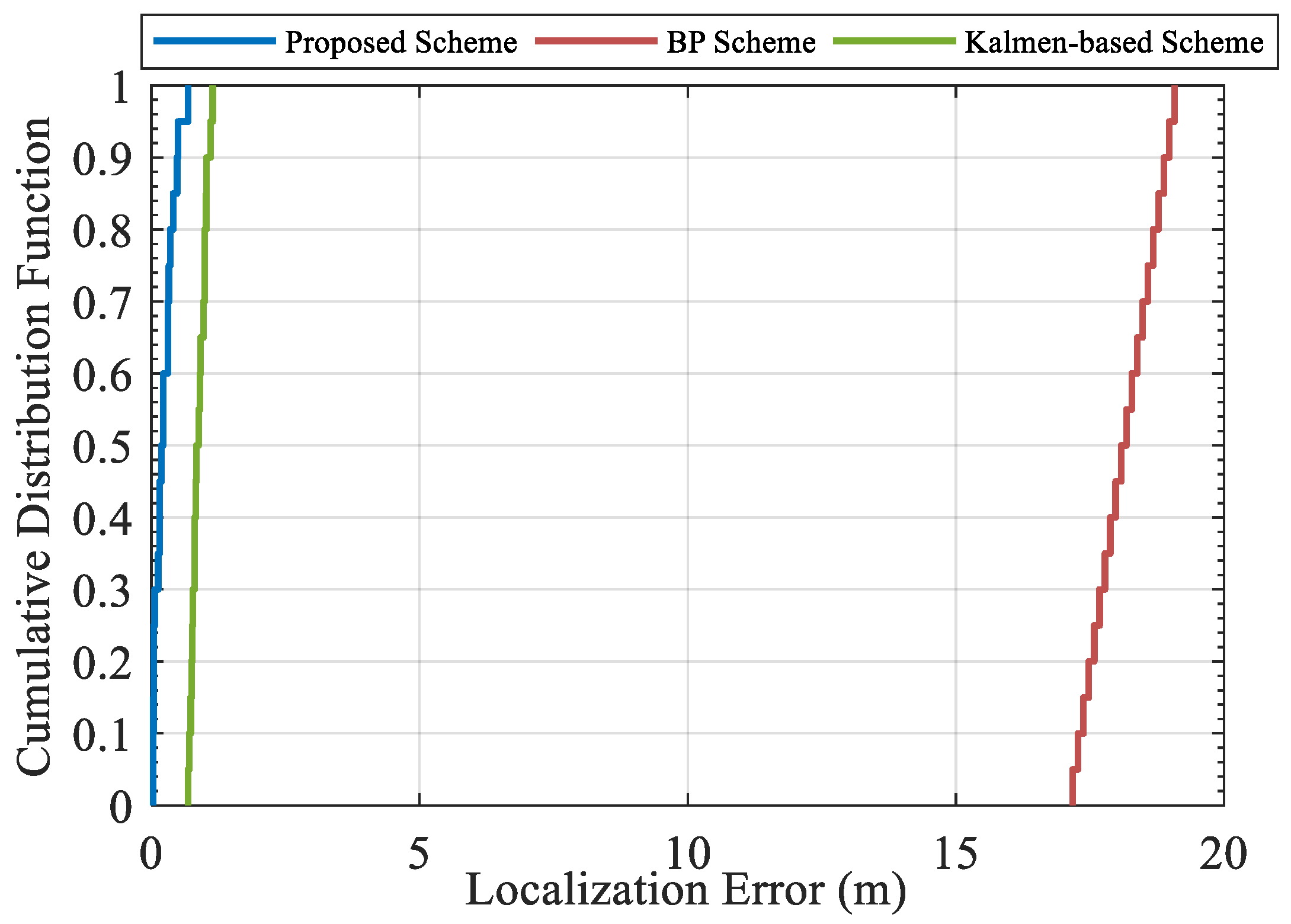
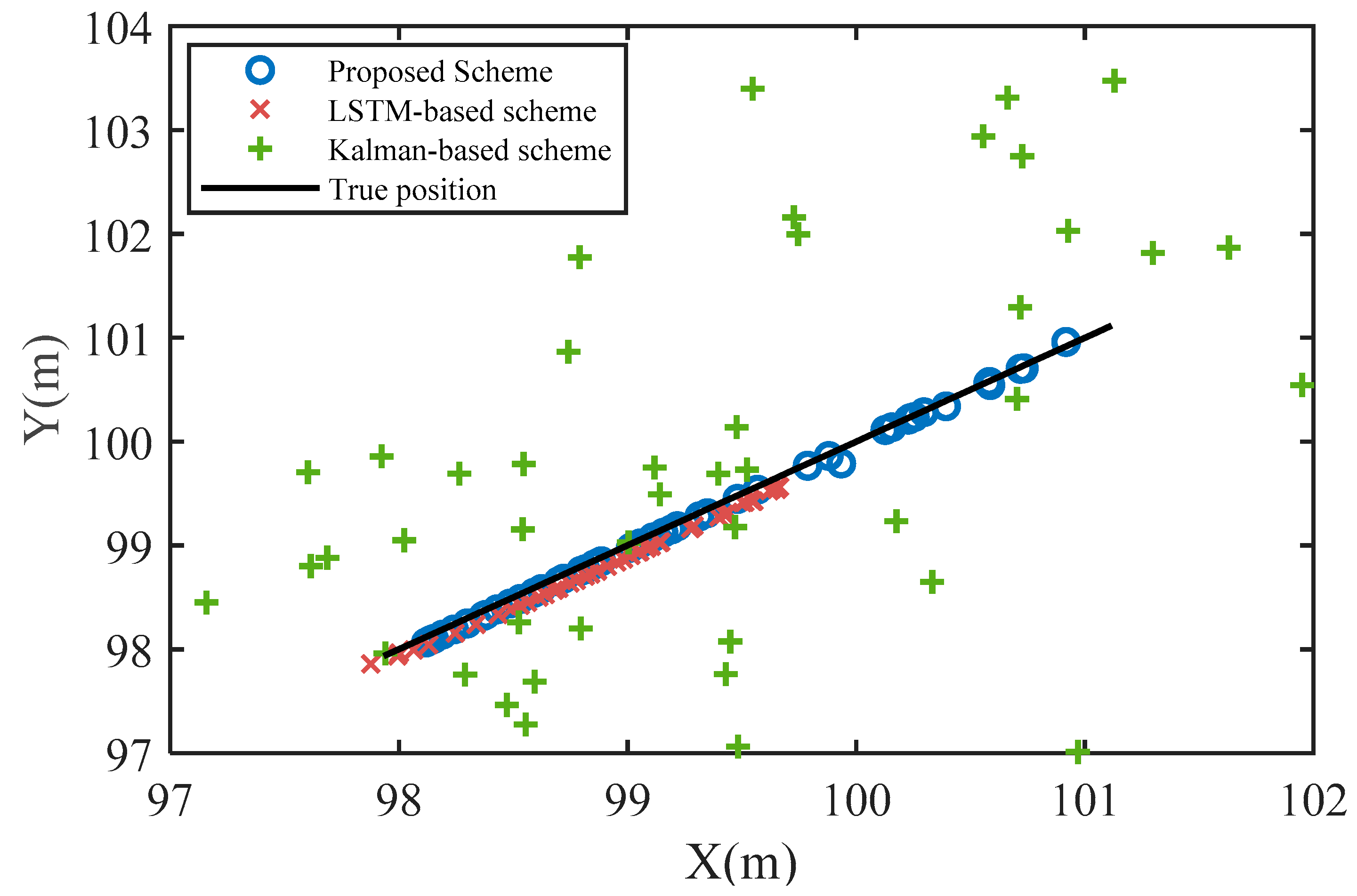
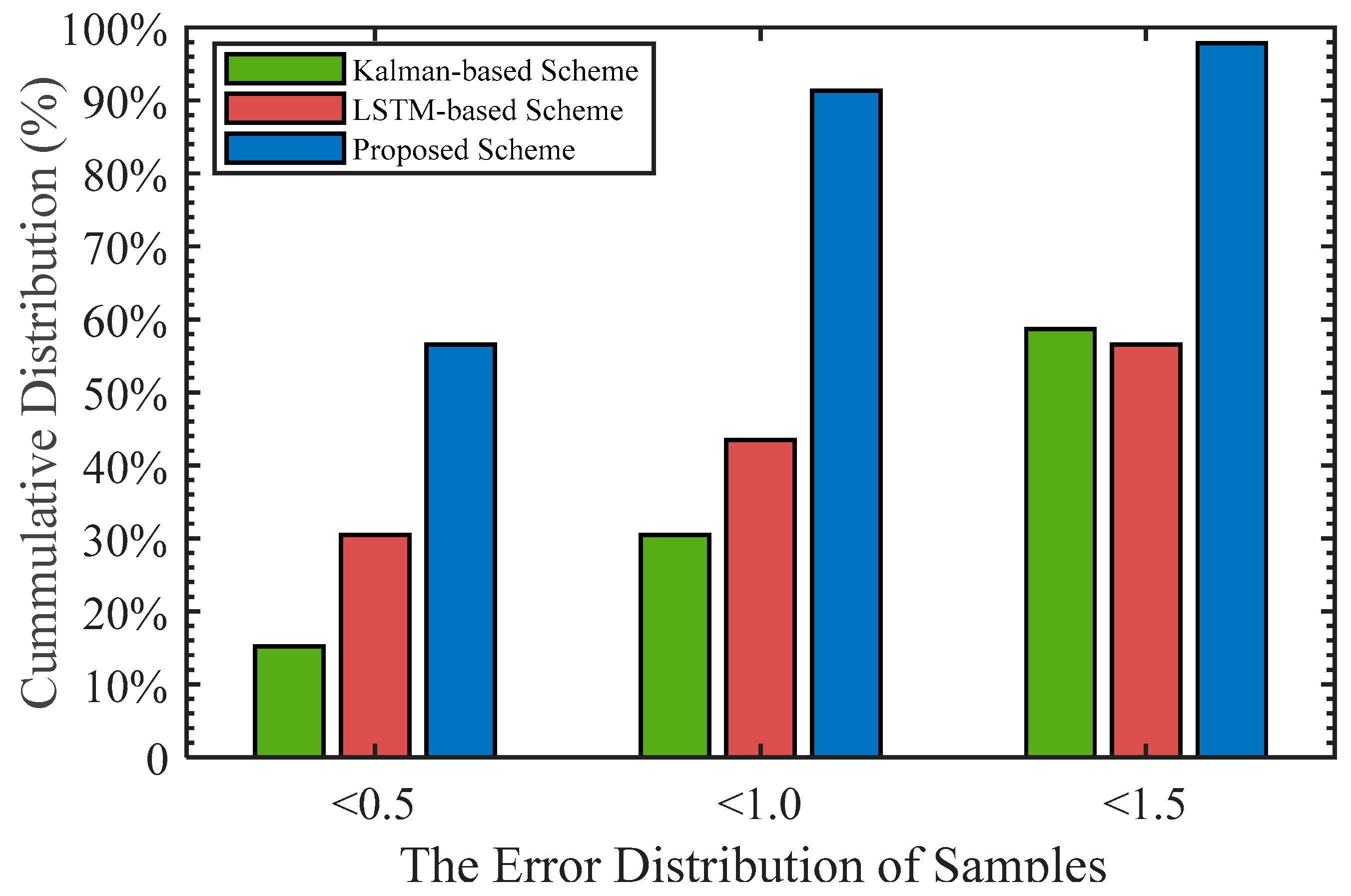
4.1. Analysis of the Localization Scheme

The simulations considered a scenario composed of 13 fixed anchors (RSUs), 99 randomly static agents (vehicles), and a mobile agent that followed in a 100 × 100 m2 line-of-sight (LOS) environment [10,12]. The remaining settings are described as follows: The maximum communication range was 20 m. The prior distribution for agents obeyed a Gaussian distribution with variances of 10 m. The driving noise vector was assumed to be Σ u k = 1 × 10 4 . The velocity of the mobile agent was uniformly generated by 0.75 m/s. Since the QPSO–BiLSTM algorithm should learn the movement trajectory of the agent, the elapsed time N was set to 1400 s. The variance of the range measurement was σ d = 1   m . In addition, the maximum number of iterations Niter was set to 4. In the simulations, the proposed localization scheme was compared with the BP algorithm with 2000 particles [12] and the Kalman-based scheme, which is a posterior linearization BP algorithm with 1/3 weight [14].
Additionally, the temporal split program was selected to split the total number of samples in agent tracking into 80% for training, 10% for validation, and 10% for testing/prediction, according to the cross-validation [29]. In the QPSO algorithm, we set the dimension to 4, the number of particles to 10, and the number of iterations to 50. The boundary conditions of the search are mentioned in Table 2.
The performance of the proposed scheme and other considerations are presented in Figure 4. The root-mean-square error (RMSE) and mean absolute error (MAE) performance indicators for evaluating the proposed localization scheme performance were selected, as suggested by [16]. The BP method lacked localization accuracy, compared with the Kalman-based scheme and the proposed scheme. Conversely, the proposed method performed well, with an RMSE of 0.23 m over 20 s. Similarly, the error of the proposed scheme was reduced by 73.8%, compared with the Kalman-based method. Specifically, in the BP method, since the number of neighbors was 2, the RMSE value was 18.12 m. The proposed localization scheme reduced the error by 98.7%, compared with the BP method. It is worth noting that the results demonstrate that the proposed localization scheme performed conspicuously in the considered scenario.
Figure 5 illustrates the cumulative distribution function (CDF) of the estimated positioning errors for the proposed and conventional localization schemes. An inspection of the presented findings indicated that the proposed method enhanced the accuracy of the results and reduced localization error, compared with other models. The error was greater with the BP method, compared with the localization results of the Kalman-based scheme and the proposed scheme. The Kalman-based method performed better, compared with the BP method, but their localization error values were greater, compared with the proposed scheme. Figure 5 shows that the proposed method performed well.

4.2. Impact of Sensor Performance on Localization Scheme

In vehicle networks, the system with sensors is affected by sensor performance [34]. In the proposed localization scheme, the sensor performance mainly affects the accuracy of the tracking algorithm. Specifically, the detection probability and false positives of the sensor mean that there are missing and outliers in the data received by the sensor. Neural networks learn and fit the input data iteratively, so a small number of missing and outliers have no impact on the tracking algorithm.
The estimated error and quality of the sensor affect the accuracy of sensor data. Furthermore, the number of sensors affects the input parameters of the proposed trajectory tracking algorithm. Therefore, we simulated the impact of the above problems on the performance of the proposed trajectory tracking algorithm. The simulation time was 50 s, in which 45 s of trajectory were training data and 5 s were testing data. The speed of the vehicle was 1 m/s.
Table 3 shows the tracking performance with different inputs. In the proposed scheme, the time, angle, speed, and the cooperative localization’s result of the vehicle are the standard input of the tracking algorithm, and the RMSE result is 0.4188 m. When the number of sensors is insufficient, the tracking accuracy without the angle sensor or the speed sensor is poorer than the standard input. Moreover, the results of RMSE are 0.4369 m and 0.4454 m, respectively. Similarly, while the speed sensor quality is inferior and has a 10% error, the tracking accuracy relatively suffers.
Furthermore, the sampling interval affects the training data for the trajectory tracking algorithm. Table 4 shows the tracking performance with different sampling frequencies. High sampling frequency means that the localization scheme has precise positioning results and a large amount of data for the tracking algorithm. However, high-frequency sampling in practice results in heavy communication overhead for the cooperative localization algorithm and even causes network congestion. Therefore, a low sampling frequency with negligible error is necessary for the cooperative localization scheme.
Although more input of localization-related sensor data is beneficial for better tracking accuracy, it is also tolerable with a small amount of missing sensor data, poor sensor accuracy, and low sampling frequency.

5. Discussion

The tracking algorithm has a significant role in localization performance in the proposed localization scheme. Here, we discuss and analyze the localization performance with different tracking algorithms composed of LSTM-based and proposed schemes. The velocity of the mobile agent was 1 m/s. The other parameters of the simulation were equivalent to those in Section 4.1. The agent node’s movement position is presented in Figure 6.
The RMSE and MAE values of the proposed scheme, Kalman-based model, and LSTM-based model considered in the comparison are summarized in Table 5. The RMSE and MAE results in the proposed scheme are less than those of the Kalman scheme and LSTM scheme, respectively, at 0.36 m and 0.51 m; in contrast, the Kalman-based values are 1.09 m and 1.57 m, respectively. Similarly, the proposed scheme reduced the RMSE values by 60% and 66.7%, compared with the LSTM-based algorithm and BP algorithm, respectively. In addition, the results obtained with the Kalman scheme are quite low, compared with the proposed method and LSTM-based method. Table 5 shows that the proposed method performed well.
Similarly, the statistics of the verification sample error from different modes are accumulated in Figure 7. The performance of the Kalman-based method is low, compared with the proposed localization scheme. In particular, the error of the proposed method is less than 1 m, at a 90% probability. It is evident from the results that the proposed model performed well, compared with the considered model.

6. Conclusions

In this paper, we focused on the limitation of cooperative localization in the number of neighbors and propose a localization scheme based on a tracing algorithm. Specifically, we employed the BP algorithm to locate the position of vehicles with a sufficient number of neighbors. Considering that the number of neighbors affects the localization accuracy of the vehicles when the number of neighbors is less than 3, we established the results of the BP algorithm as historical position values and further developed a QPSO–BiLSTM model to precisely predict the positions of agents. A fundamental advantage of the proposed cooperative localization scheme over classic cooperative localization is that agents have stable localization accuracy. In addition, the proposed cooperative localization scheme solves the problem of relying on the distribution of neighbors, which is useful for the localization of ITSs.

Author Contributions

Conceptualization, T.Y.; methodology, T.Y.; software, T.Y.; validation, C.B., D.Z. and X.L.; formal analysis, T.Y.; writing—original draft preparation, T.Y.; writing—review and editing, C.B.; supervision, D.Z.; and funding acquisition, D.Z. All authors have read and agreed to the published version of the manuscript.

Funding

This research is supported by the National Natural Science Foundation of China under Grant No 41974032.

Data Availability Statement

The data used to support the findings of this study are available from the corresponding author upon request.

Conflicts of Interest

The authors declare no conflict of interest.

References

  1. Chandra Shit, R. Crowd intelligence for sustainable futuristic intelligent transportation system: A review. IET Intell. Transp. Syst. 2020, 14, 480–494. [Google Scholar] [CrossRef]
  2. Wymeersch, H.; Seco-Granados, G.; Destino, G.; Dardari, D.; Tufvesson, F. 5G mmWave Positioning for Vehicular Networks. IEEE Wire. Commun. 2017, 24, 80–86. [Google Scholar] [CrossRef] [Green Version]
  3. Sharma, S.; Bhatia, V.; Gupta, A. Sparsity based narrowband interference mitigation in UWB communication for 5G and beyond. Elsevier Comput. Electr. Eng. 2017, 64, 83–95. [Google Scholar] [CrossRef]
  4. Sharma, S.; Bhatia, V.; Gupta, A. Joint Symbol and ToA Estimation for Iterative Transmitted Reference Pulse Cluster UWB System. IEEE Syst. J. 2019, 13, 2629–2640. [Google Scholar] [CrossRef]
  5. Va, V.; Shimizu, T.; Bansal, G.; Heath, R.W. Millimeter Wave Vehicular Communications: A Survey. Found. Trends Netw. 2016, 10, 1–113. [Google Scholar] [CrossRef]
  6. Piccinni, G.; Avitabile, G.; Coviello, G. An improved technique based on Zadoff-Chu sequences for distance measurements. In Proceedings of the 2016 IEEE Radio and Antenna Days of the Indian Ocean (RADIO), Reunion, France, 10–13 October 2016. [Google Scholar]
  7. Fadzilla, M.A.; Harun, A.; Shahriman, A.B. Localization Assessment for Asset Tracking Deployment by Comparing an Indoor Localization System with a Possible Outdoor Localization System. In Proceedings of the 2018 International Conference on Computational Approach in Smart Systems Design and Applications (ICASSDA), Kuching, Malaysia, 15–17 August 2018. [Google Scholar]
  8. Ammous, M.; Valaee, S. Cooperative Positioning in Vehicular Networks using Angle of Arrival Estimation through mmWave. In Proceedings of the GLOBECOM, Madrid, Spain, 7–11 December 2020. [Google Scholar]
  9. Soatti, G.; Nicoli, M.; Garcia, N.; Denis, B.; Raulefs, R.; Wymeersch, H. Implicit Cooperative Positioning in Vehicular Networks. IEEE Trans. Intell. Transp. Syst. 2018, 19, 3964–3980. [Google Scholar] [CrossRef] [Green Version]
  10. Seco, F.; Jiménez, A.; Zheng, X. RFID-based centralized cooperative localization in indoor environments. In Proceedings of the IPIN 2016: International Conference on Indoor Positioning and Indoor Navigation, Madrid, Spain, 4–7 October 2016. [Google Scholar]
  11. Ihler, A.T.; Fisher, J.W.; Moses, R.L.; Willsky, A.S. Nonparametric belief propagation for self-localization of sensor networks. In Proceedings of the 3rd International Symposium on Information Processing in Sensor Networks, Berkeley, CA, USA, 26–27 April 2004. [Google Scholar]
  12. Wymeersch, H.; Lien, J.; Win, M.Z. Cooperative Localization in Wireless Networks. Proc. IEEE 2009, 97, 427–450. [Google Scholar] [CrossRef]
  13. Pedersen, C.; Pedersen, T.; Fleury, B.H. A Variational Message Passing Algorithm for Sensor Self-Localization in Wireless Networks. In Proceedings of the IEEE International Symposium on Information Theory Proceedings (ISIT), St Petersburg, Russia, 31 July–5 August 2011. [Google Scholar]
  14. Garcia-Fernandez, A.F.; Svensson, L.; Sarkka, S. Cooperative Localization Using Posterior Linearization Belief Propagation. IEEE Trans. Veh. Technol. 2018, 67, 832–836. [Google Scholar] [CrossRef]
  15. Cakmak, B.; Urup, D.N.; Meyer, F.; Pedersen, T.; Fleury, B.H.; Hlawatsch, F. Cooperative Localization for Mobile Networks: A Distributed Belief Propagation—Mean Field Message Passing Algorithm. IEEE Signal Process. Lett. 2016, 23, 828–832. [Google Scholar] [CrossRef] [Green Version]
  16. Hehdly, K.; Laaraiedh, M.; Abdelkefi, F.; Siala, M. Cooperative localization and tracking in wireless sensor networks. Int. J. Commun. Syst. 2018, 32, e3842. [Google Scholar] [CrossRef] [Green Version]
  17. Meyer, F.; Hlinka, O.; Wymeersch, H.; Riegler, E.; Hlawatsch, F. Distributed Localization and Tracking of Mobile Networks Including Noncooperative Objects. IEEE Trans. Signal Inform. Process. Netw. 2016, 2, 57–71. [Google Scholar] [CrossRef] [Green Version]
  18. Meyer, F.; Riegler, E.; Hlinka, O.; Hlawatsch, F. Simultaneous Distributed Sensor Self-Localization and Target Tracking Using Belief Propagation and Likelihood Consensus. In Proceedings of the 2012 Conference Record of The Forty Sixth Asilomar Conference on Signals, Systems and Computers (ASILOMAR), Pacific Grove, CA, USA, 4–7 November 2012. [Google Scholar]
  19. Meyer, F.; Hlawatsch, F.; Wymeersch, H. Cooperative simultaneous localization and tracking (coslat) with reduced complexity and communication. In Proceedings of the ICASSP, Pacific Grove, CA, USA, 4–7 November 2012. [Google Scholar]
  20. Eom, J.; Kim, H.; Lee, S.H.; Kim, S. DNN-Assisted Cooperative Localization in Vehicular Networks. Energies 2019, 12, 2758. [Google Scholar] [CrossRef] [Green Version]
  21. Kim, H.; Granstrom, K.; Gao, L.; Battistelli, G.; Kim, S.; Wymeersch, H. 5G mmWave Cooperative Positioning and Mapping using Multi-Model PHD Filter and Map Fusion. IEEE Trans. Wirel. Commun. 2019, 16, 3782–3795. [Google Scholar] [CrossRef] [Green Version]
  22. Denis, B.; Maman, M.; Ouvry, L. On the scheduling of ranging and distributed positioning updates in cooperative IR-UWB networks. In Proceedings of the IEEE International Conference on Ultra-Wideband, Vancouver, BC, Canada, 9–11 September 2009. [Google Scholar]
  23. Zhang, R.; Zhao, Z.; Cheng, X.; Yang, L. Overlapping Coalition Formation Game Based Opportunistic Cooperative Localization Schemefor Wireless Networks. IEEE Trans. Commun. 2017, 65, 3629–3642. [Google Scholar]
  24. Sathyan, T.; Hedley, M. Fast and Accurate Cooperative Tracking in Wireless Networks. IEEE Trans. Mob. Comput. 2013, 12, 1801–1813. [Google Scholar] [CrossRef]
  25. Tian, Q.; Wang, K.I.-K.; Salcic, Z. A Resetting Approach for INS and UWB Sensor Fusion Using Particle Filter for Pedestrian Tracking. IEEE Trans. Instrum. Meas. 2020, 69, 5914–5921. [Google Scholar] [CrossRef]
  26. Tian, Q.; Wang, K.I.-K.; Salcic, Z. An INS and UWB Fusion Approach with Adaptive Ranging Error Mitigation for Pedestrian Tracking. IEEE Sens. J. 2020, 20, 4372–4381. [Google Scholar] [CrossRef]
  27. Alvarez-Merino, C.S.; Luo-Chen, H.Q.; Khatib, E.J.; Barco, R. Opportunistic Fusion of Ranges from Different Sources for Indoor Positioning. IEEE Commun. Lett. 2021, 25, 2260–2264. [Google Scholar] [CrossRef]
  28. Zhang, M.; Jia, J.; Chen, J.; Deng, Y.; Wang, X.; Aghvami, A.H. Indoor Localization Fusing WiFi with Smartphone Inertial Sensors Using LSTM Networks. IEEE Internet Things J. 2021, 8, 13608–13623. [Google Scholar] [CrossRef]
  29. Llinas, J.; Antony, R.T. Blackboard Concepts for Data Fusion Applications. Int. J. Pattern Recognit. Artif. Intell. 1993, 7, 285–308. [Google Scholar] [CrossRef]
  30. Graves, A.; Schmidhuber, J. Framewise phoneme classification with bidirectional LSTM and other neural network architectures. Neural Netw. 2005, 18, 602–610. [Google Scholar] [CrossRef] [PubMed]
  31. Greff, K.; Srivastava, R.K.; Koutník, J.; Steunebrink, B.R.; Schmidhuber, J. LSTM: A Search Space Odyssey. IEEE Trans. Neural Netw. Learn. Syst. 2016, 28, 2222–2232. [Google Scholar] [CrossRef] [PubMed] [Green Version]
  32. Omkar, S.; Khandelwal, R.; Ananth, T.; Naik, G.N.; Gopalakrishnan, S. Quantum behaved Particle Swarm Optimization (QPSO) for multi-objective design optimization of composite structures. Expert Syst. Appl. Int. J. 2009, 36, 11312–11322. [Google Scholar] [CrossRef]
  33. Sun, J.; Xu, W.; Feng, B. A global search strategy of quantum-behaved particle swarm optimization. In Proceedings of the IEEE Conference on Cybernetics and Intelligent Systems, Singapore, 1–3 December 2004. [Google Scholar]
  34. Sharma, S.; Gupta, A.; Bhatia, V. IR-UWB Sensor Network Using Massive MIMO Decision Fusion: Design and Performance Analysis. IEEE Sens. J. 2018, 18, 6290–6302. [Google Scholar] [CrossRef]
Figure 1. Illustration of the localization system.
Electronics 11 00603 g001
Figure 2. Factor graph showing the state of agents from time (n − 1) to time n.
Electronics 11 00603 g002
Figure 3. BiLSTM architecture.
Electronics 11 00603 g003
Figure 4. RMSE for the localization scheme.
Electronics 11 00603 g004
Figure 5. Cumulative distribution function for positioning error.
Electronics 11 00603 g005
Figure 6. Agent’s movement position.
Electronics 11 00603 g006
Figure 7. Agents’ movement positions.
Electronics 11 00603 g007
Table 1. Parameters of different sensors.
5GVehicle Information
Sensor 1Angle, Time, Position-
Sensor 2-Velocity
Table 2. Limited conditions of optimized parameters for QPSO–BiLSTM.
Hidden Layer 1Hidden Layer 2Learning RateMax Epochs
maximum2502500.1200
minimum110.0011
Table 3. The tracking performance with different inputs.
The Standard InputWithout the
Angle Sensor
Without the Speed SensorWith Poor
Speed Sensor
RMSE0.4188 m0.4369 m0.4454 m0.4347 m
Table 4. The tracking performance with different sampling frequencies.
20 Hz10 Hz8 Hz
RMSE0.4188 m0.4369 m0.4454 m
Table 5. Performance of the localization scheme for different tracking models.
Kalman-BasedLSTM-BasedProposed Scheme
RMSE1.0946 m0.9030 m0.3628 m
MAE1.5717 m1.2682 m0.5102 m
Publisher’s Note: MDPI stays neutral with regard to jurisdictional claims in published maps and institutional affiliations.

