Cascaded RLS Adaptive Filters Based on a Kronecker Product Decomposition

Abstract

The multilinear system framework allows for the exploitation of the system identification problem from different perspectives in the context of various applications, such as nonlinear acoustic echo cancellation, multi-party audio conferencing, and video conferencing, in which the system could be modeled through parallel or cascaded filters. In this paper, we introduce different memoryless and memory structures that are described from a bilinear perspective. Following the memory structures, we develop the multilinear recursive least-squares algorithm by considering the Kronecker product decomposition concept. We have performed a set of simulations in the context of echo cancellation, aiming both long length impulse responses and the reverberation effect.

1. Introduction

In the field of system identification, many applications involve adaptive filtering algorithms [1,2]. One of them is the echo cancellation problem, which has raised many challenges over the years [3,4]. Based on the input-output relation, a dynamic system should be determined (i.e., the echo path), considering various parameters and external factors that must be estimated. These dynamic systems are modeled linearly through an adaptive filter with a finite-impulse-response (FIR) structure [5,6]. The main performance bottlenecks, in terms of computational complexity, tracking, and convergence rate, arise when the length of the impulse response reaches hundreds/thousands of coefficients. The literature presents many approaches to improve the overall performance, also taking into account the fact that the echo paths are sparse in nature [7,8,9,10,11,12,13]. Recently, in our previous work [14], we introduced a new approach of splitting a long length impulse response into several impulse responses of shorter lengths, aiming to reduce the computational complexity by maintaining the overall performance. Another challenge arises when the echo path produces multiple reflections, and this effect is called reverberation. From a mathematical point of view, this effect could be described (to some extent) by using the Kronecker product decomposition of the impulse response [15,16].

In this paper, we extend our study on cascaded adaptive filters, aiming to reduce the computational complexity considering both long length impulse responses and the reverberation effect. Our approach is based on multilinear structures and the Kronecker product decomposition. The main goal is to outline the features of this development and its potential.

The rest of the paper is organized as follows. Section 2 presents the background for different bilinear structures without memory, while Section 3 introduces bilinear structures with memory. In Section 4, the new development is combined with the recursive least-squares (RLS) algorithm, thus resulting in a practical solution based on adaptive filtering. We perform an experimental study in Section 5 and conclude the paper in Section 6.

2. Bilinear Structures without Memory

In order to introduce the bilinear structures with memory and the development based on the Kronecker product decomposition, let us start by presenting the bilinear structure without memory [14,17,18], defined as

$$\begin{array}{cc}\hfill y\left(n\right)& ={\mathbf{h}}_1^T\mathbf{X}\left(n\right){\mathbf{h}}_2=\sum _{l_1=1}^{L_1}\sum _{l_2=1}^{L_2}{x}_{l_1{l}_2}\left(n\right)h_{1,l_1}{h}_{2,l_2},\hfill \end{array}$$

(1)

where $\mathbf{X}\left(n\right)$ is the multiple input data matrix of size $L_1\times L_2$, with

$$\begin{array}{c}\hfill \mathbf{X}\left(n\right)=\left[\begin{array}{ccccc}{\mathbf{x}}_1\left(n\right)& \cdots & {\mathbf{x}}_{l_2}\left(n\right)& \cdots & {\mathbf{x}}_{L_2}\left(n\right)\end{array}\right],\end{array}$$

(2)

and

$$\begin{array}{c}\hfill {\mathbf{x}}_{l_2}\left(n\right)={\left[\begin{array}{ccccc}{x}_{l_2,1}\left(n\right)& \cdots & x_{l_2,l_1}\left(n\right)& \cdots & x_{l_2,L_1}\left(n\right)\end{array}\right]}^T,l_2=1,2,\dots ,L_2\end{array}$$

(3)

is an input signal vector containing the $L_1$ most recent data at the discrete-time index n, while the superscript ^T is the transpose operator. The two impulse responses ${\mathbf{h}}_1$ and ${\mathbf{h}}_2$ have $L_1$ and $L_2$ coefficients, respectively. In other words, the input-output equation in (1) describes a system with $L_1{L}_2$ inputs and a single output. In order to facilitate the graphical representation, let us rewrite (1) as

$$\begin{array}{cc}\hfill y\left(n\right)& =\sum _{l_1=1}^{L_1}{h}_{1,l_1}\sum _{l_2=1}^{L_2}{h}_{2,l_2}{x}_{l_1{l}_2}\left(n\right)=\sum _{l_2=1}^{L_2}{h}_{2,l_2}\sum _{l_1=1}^{L_1}{h}_{1,l_1}{x}_{l_1{l}_2}\left(n\right)\hfill \\ \hfill & =\sum _{l_2=1}^{L_2}{h}_{2,l_2}{s}_{1,l_2}\left(n\right),\hfill \end{array}$$

(4)

where

$$\begin{array}{c}\hfill s_{1,l_2}\left(n\right)=\sum _{l_1=1}^{L_1}{h}_{1,l_1}{x}_{l_1{l}_2}\left(n\right)\end{array}$$

(5)

is the output of a memoryless weighted adder with $L_1$ inputs at the discrete-time index n. We can transpose (5) in a graphical representation as shown in Figure 1.

Based on (4) and Figure 1, we can introduce the graphical respresentation of the multiple-input single-output (MISO) system as shown in Figure 2. Overall, this structure consists of two levels of combiners.

3. Bilinear Structures with Memory

By introducing a delay line, the $s_{1,l_2}\left(n\right)$ structure described by $L_1$ inputs and a single output can be transformed in a single-input single-output (SISO) structure. Therefore, the following input signal vector results

$$\begin{array}{c}\hfill {\mathbf{x}}_{l_2}\left(n\right)={\left[\begin{array}{ccccc}{x}_{l_2}\left(n\right)& \cdots & x_{l_2}(n-l_1+1)& \cdots & x_{l_2}(n-L_1+1)\end{array}\right]}^T,l_2=1,2,\dots ,L_2.\end{array}$$

(6)

Thus, the input data matrix has the following structure:

$$\mathbf{X}\left(n\right)=\left[\begin{array}{ccccc}{x}_1\left(n\right)& \cdots & x_{l_2}\left(n\right)& \cdots & x_{L_2}\left(n\right)\\ x_1(n-1)& \cdots & x_{l_2}(n-1)& \cdots & x_{L_2}(n-1)\\ ⋮& \ddots & ⋮& \ddots & ⋮\\ x_1(n-L_1+1)& \cdots & x_{l_2}(n-L_1+1)& \cdots & x_{L_2}(n-L_1+1)\end{array}\right].$$

Hence,

$$\begin{array}{c}\hfill s_{1,l_2}\left(n\right)=\sum _{l_1=1}^{L_1}{h}_{1,l_1}{x}_{l_2}(n-l_1+1)\end{array}$$

(7)

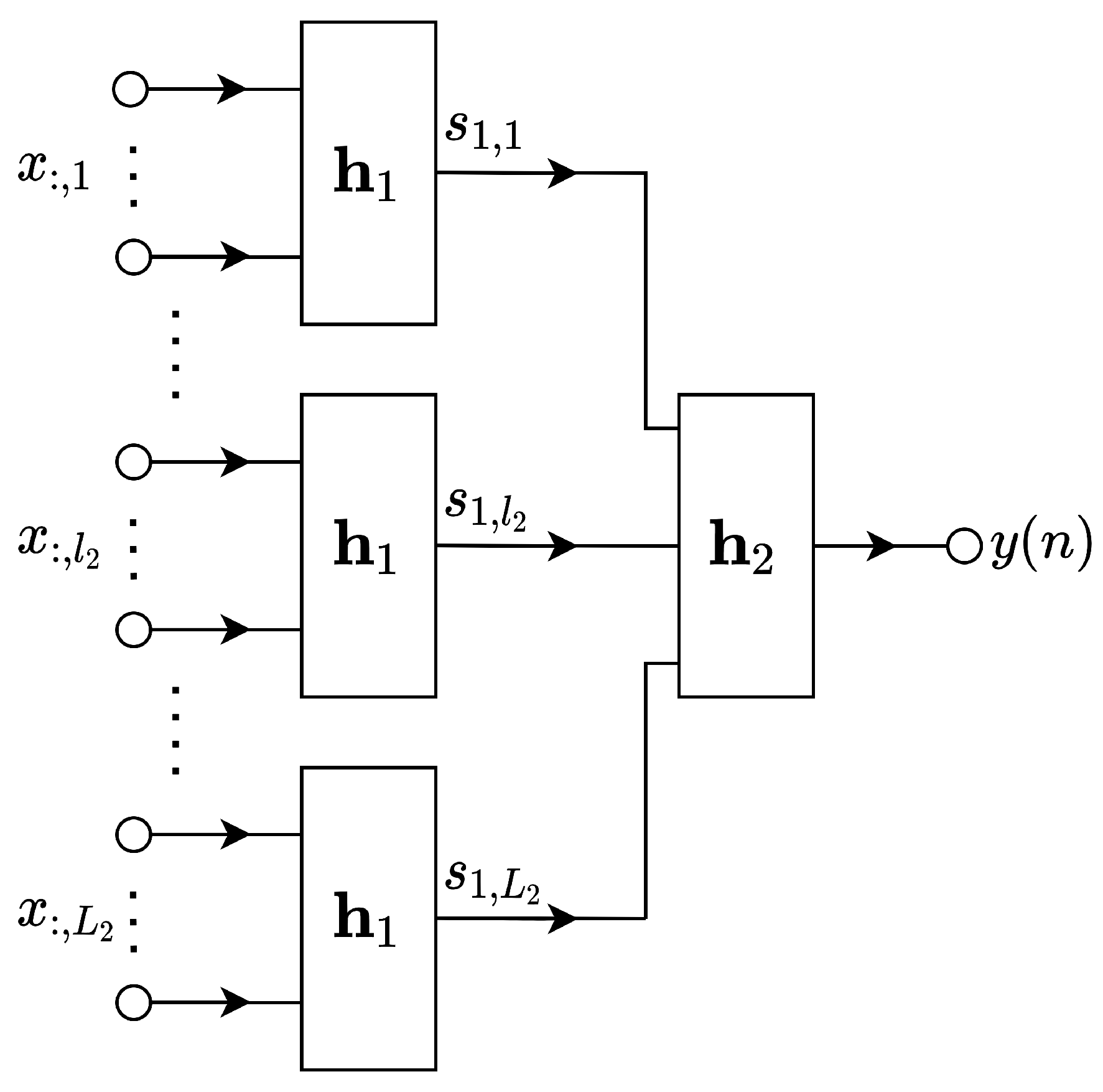
is a structure associated to a transversal filter, with the weighted function ${\mathbf{h}}_1$, having as input the vector ${\mathbf{x}}_{l_2}\left(n\right)$. The graph representation of the new $s_{1,l_2}\left(n\right)$ structure is shown in Figure 3. Also, Figure 4 outlines the two combiner level structures based on the transversal filters.

In terms of the z-transform, (7) is defined as

$$\begin{array}{cc}\hfill S_{1,l_2}\left(z\right)& =\sum _{n=-\infty }^{\infty }{s}_{1,l_2}\left(n\right)z^{-n}=\sum _{l_1=1}^{L_1}{h}_{1,l_1}\sum _{n=-\infty }^{\infty }{x}_{l_2}(n-l_1+1)z^{-n}\hfill \\ \hfill & =X_{l_2}\left(z\right)\sum _{l_1=1}^{L_1}{h}_{1,l_1}{z}^{-l_1+1}\hfill \\ \hfill & =X_{l_2}\left(z\right)H_1\left(z\right),\hfill \end{array}$$

(8)

where

$$\begin{array}{c}\hfill H_1\left(z\right)=\sum _{l_1=1}^{L_1}{h}_{1,l_1}{z}^{-l_1+1}.\end{array}$$

(9)

A more efficient form in terms of correlation between the columns of the input matrix $\mathbf{X}\left(n\right)$ can be obtained if we consider successive data related to the columns, and is defined as

$$\mathbf{X}(n)=\left[\begin{array}{ccccc}{x}_1\left(n\right)& \cdots & x_1(n-(l_2-1)L_1)& \cdots & x_1(n-(L_2-1)L_1)\\ x_1(n-1)& \cdots & x_1(n-(l_2-1)L_1-1)& \cdots & x_1(n-(L_2-1)L_1-1)\\ ⋮& \ddots & ⋮& \ddots & ⋮\\ x_1(n-L_1+1)& \cdots & x_1(n-(l_2-1)L_1-L_1+1)& \cdots & x_1(n-(L_2-1)L_1-L_1+1)\end{array}\right].$$

The input signal vector becomes a sequence of $L_1{L}_2$ successive data applied to a FIR filter of length $L_1{L}_2$, so that

$$\begin{array}{c}\hfill \mathbf{x}\left(n\right)=\mathrm{vec}\left[\mathbf{X}\right(n\left)\right],\end{array}$$

(10)

where $\mathrm{vec}(·)$ denotes the vectorization operation and

$$\begin{array}{c}\hfill s_{1,l_2}\left(n\right)=\sum _{l_1=1}^{L_1}{h}_{1,l_1}{x}_1(n-l_1{L}_2),\end{array}$$

(11)

with $x_1\left(n\right)=x_1(n-L_1),\dots ,x_{l_2}\left(n\right)=x_1(n-l_1{L}_2),\dots ,x_{L_2}\left(n\right)=x_1(n-L_1{L}_2)$. In terms of the z-transform, we can write (11) as

$$\begin{array}{cc}\hfill S_{1,l_2}\left(z\right)& =\sum _{l_1=1}^{L_1}{X}_1\left(z\right)z^{-l_1{L}_2}{h}_{1,l_1}\hfill \\ \hfill & =X_1\left(z\right)\sum _{l_1=1}^{L_1}{z}^{-l_1{L}_2}{h}_{1,l_1}=X_1\left(z\right)H_1\left(z^{L_2}\right).\hfill \end{array}$$

(12)

Forwards, the output of the global system in the z-transform domain is

$$\begin{array}{c}\hfill Y\left(z\right)=S_{1,l_2}\left(z\right)H_2\left(z\right)=X_1\left(z\right)H_1\left(z^{L_2}\right)H_2\left(z\right)=X_1\left(z\right)H\left(z\right),\end{array}$$

(13)

where

$$\begin{array}{c}\hfill H\left(z\right)=H_1\left(z^{L_2}\right)H_2\left(z\right).\end{array}$$

(14)

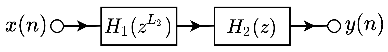
Equation (12) describes a SISO structure of two cascaded filters as shown in Figure 5. The first filter $H_1\left(z^{L_2}\right)$ is obtained through interpolation with zeroes by $L_2$ factor of the $H_1\left(z\right)$ function and its length is $L_2(L_1-1)+1$. Indeed, it has only $L_1$ non-zero coefficients, from the total of $L_2(L_1-1)+1$, (hence a certain degree of sparsity), according to its impulse response

$$\begin{array}{c}\hfill {\mathbf{h}}_1^{{}^{\prime }}\left(n\right)=\left\{\begin{array}{cc}{\mathbf{h}}_1\left(\frac{n}{L_1}\right),\hfill & \mathrm{for}n\mathrm{mod}{L}_1=0,n=1,2,\dots ,L_2(L_1-1)+1\hfill \\ 0,\hfill & \mathrm{otherwise}\hfill \end{array}\right.,\end{array}$$

(15)

where ${\mathbf{h}}_1^{{}^{\prime }}\left(n\right)$ is the impulse response of $H_1\left(z^{L_2}\right)$ and $\mathrm{mod}$ denotes the modulo operation. The second filter, $H_2\left(z\right)$, is of length $L_2$. Afterwards, the total length of the $H\left(z\right)$ filter is $L_2(L_1-1)+1+L_2-1=L_1{L}_2$.

Based on this configuration, let us consider the two vectors:

$${\mathbf{h}}_1=\left[\begin{array}{c}{h}_{1,1}\\ h_{1,2}\\ ⋮\\ h_{1,l_1}\\ ⋮\\ h_{1,L_1}\end{array}\right],{\mathbf{h}}_2=\left[\begin{array}{c}{h}_{2,1}\\ h_{2,2}\\ ⋮\\ h_{2,l_2}\\ ⋮\\ h_{2,L_2}\end{array}\right],$$

and the Kronecker product:

$$\mathbf{h}={\mathbf{h}}_1\otimes {\mathbf{h}}_2=\left[\begin{array}{c}{h}_{1,1}{\mathbf{h}}_2\\ h_{1,2}{\mathbf{h}}_2\\ ⋮\\ h_{1,l_1}{\mathbf{h}}_2\\ ⋮\\ h_{1,L_1}{\mathbf{h}}_2\end{array}\right].$$

Having as coefficients the elements of this vector, the polynomial form is developed as

$$\begin{array}{c}\hfill H\left(z\right)=\sum _{r=0}^{L_1{L}_2-1}{h}_r{z}^{-r}\end{array}$$

(16)

and can be factored in the form described in (14). While the position of an element for the $l_1,l_2$ indexes is $r=(l_1-1)L_2+l_2-1$, we have

$$\begin{array}{cc}\hfill H_1\left(z^{L_2}\right)H_2\left(z\right)& =\sum _{l_1=1}^{L_1}{h}_{1,l_1}{z}^{-(l_1-1)L_2}\sum _{l_2=1}^{L_2}{h}_{2,l_2}{z}^{-(l_2-1)}\hfill \\ \hfill & =\sum _{l_1=1}^{L_1}\sum _{l_2=1}^{L_2}{h}_{1,l_1}{h}_{2,l_2}{z}^{-(l_1-1)L_2-(l_2-1)}\hfill \\ \hfill & =\sum _{r=0}^{L_1{L}_2-1}{h}_r{z}^{-r}.\hfill \end{array}$$

(17)

4. Cascaded Multilinear RLS Algorithm Using Kronecker Product Decomposition

Based on the development from Section 3, we introduce the set of equations for the RLS algorithm in a multilinear manner, following the Kronecker product decomposition [14,19]. Our approach is determined considering the system identification framework. In this context, the output of the MISO system is

$$\begin{array}{c}\hfill y\left(n\right)=\mathcal{X}\left(n\right){\times }_1{\mathbf{h}}_1^T{\times }_2{\mathbf{h}}_2^T{\times }_i\cdots {\times }_N{\mathbf{h}}_N^T,\end{array}$$

(18)

where N denotes the multilinear degree and ${\times }_i$ represents the multiplication operation by the dimension $i=1,2,\dots ,N$. The input data are described in a N degree tensorial form as ${\left[\mathcal{X}\left(n\right)\right]}_{l_1{l}_2\dots l_N}$ with the real-values $x_{l_1{l}_2\dots l_N},l_i=1,2,\dots ,L_i,i=1,2,\dots ,N$. The vector ${\mathbf{h}}_i$ of length $L_i$, stores the impulse response for the i cascaded filter, $i=1,2,\dots ,N$. Based on the ${\mathbf{h}}_i$ ($i=1,2,\dots ,N$) impulse responses of the MISO system, the rank-1 tensor of dimension $L_1\times L_2\times \cdots \times L_N$ is

$$\begin{array}{c}\hfill \mathcal{H}={\mathbf{h}}_1\circ {\mathbf{h}}_2\circ \cdots \circ {\mathbf{h}}_N,\end{array}$$

(19)

where ∘ denotes the outer product. Usually, in the context of system identification, the desired signal results from the output signal corrupted by an additive noise, $w\left(n\right)$, which in our development is a zero-mean Gaussian signal, so that

$$\begin{array}{c}\hfill d\left(n\right)=y\left(n\right)+w\left(n\right).\end{array}$$

(20)

Consequently, the output signal described by (18) results in

$$\begin{array}{c}\hfill y\left(n\right)={\mathrm{vec}}^T\left[\mathcal{X}\left(n\right)\right]\mathrm{vec}\left(\mathcal{H}\right),\end{array}$$

(21)

where

$$\mathrm{vec}\left[\mathcal{X}\left(n\right)\right]=\left[\begin{array}{c}\mathrm{vec}\left[{\mathbf{X}}_{::\cdots :L_1}\left(n\right)\right]\\ \mathrm{vec}\left[{\mathbf{X}}_{::\cdots :L_2}\left(n\right)\right]\\ ⋮\\ \mathrm{vec}\left[{\mathbf{X}}_{::\cdots :L_N}\left(n\right)\right]\end{array}\right]\triangleq \tilde{\mathbf{x}}\left(n\right)$$

and

$$\mathrm{vec}\left(\mathcal{H}\right)=\left[\begin{array}{c}\mathrm{vec}\left({\mathbf{H}}_{::\cdots :L_1}\right)\\ \mathrm{vec}\left({\mathbf{H}}_{::\cdots :L_2}\right)\\ ⋮\\ \mathrm{vec}\left({\mathbf{H}}_{::\cdots :L_N}\right)\end{array}\right]={\mathbf{h}}_N\otimes \cdots \otimes {\mathbf{h}}_2\otimes {\mathbf{h}}_1\triangleq \mathbf{h},$$

with ${\mathbf{X}}_{::\cdots :l_i}\left(n\right)\in {\mathbb{R}}^{L_1\times L_2\times \cdots \times L_{N-1}}$ and ${\mathbf{H}}_{::\cdots :l_i}\left(n\right)\in {\mathbb{R}}^{L_1\times L_2\times \cdots \times L_{N-1}}$ representing the frontal slices of $\mathcal{X}\left(n\right)$ and $\mathcal{H}\left(n\right)$, respectively. The two new vectors $\tilde{\mathbf{x}}\left(n\right)$ and $\mathbf{h}$ consist of $L_1{L}_2\cdots L_N$ elements. Also, the output of the system can be rewritten as

$$\begin{array}{c}\hfill y\left(n\right)={\tilde{\mathbf{x}}}^T\left(n\right)\mathbf{h}.\end{array}$$

(22)

Then, the a priori error signal is computed as

$$\begin{array}{c}\hfill e\left(n\right)=d\left(n\right)-\widehat{y}\left(n\right),\end{array}$$

(23)

where $\widehat{y}\left(n\right)$ represents an estimate of the output signal. Following the least-squares (LS) error criterion, we can introduce the cost functions:

$$\begin{array}{cc}\hfill \mathcal{J}\left[{\widehat{\mathbf{h}}}_1\left(n\right)\right]& =\sum _{k=1}^n{\lambda }_1^{n-k}{[d\left(n\right)-{\widehat{\mathbf{h}}}_1^T\left(n\right){\tilde{\mathbf{x}}}_{{\widehat{\mathbf{h}}}_2{\widehat{\mathbf{h}}}_3\cdots {\widehat{\mathbf{h}}}_N}\left(n\right)]}^2,\hfill \\ \hfill \mathcal{J}\left[{\widehat{\mathbf{h}}}_2\left(n\right)\right]& =\sum _{k=1}^n{\lambda }_2^{n-k}{[d\left(n\right)-{\widehat{\mathbf{h}}}_2^T\left(n\right){\tilde{\mathbf{x}}}_{{\widehat{\mathbf{h}}}_1{\widehat{\mathbf{h}}}_3\cdots {\widehat{\mathbf{h}}}_N}\left(n\right)]}^2,\hfill \\ \hfill ⋮& \\ \hfill \mathcal{J}\left[{\widehat{\mathbf{h}}}_N\left(n\right)\right]& =\sum _{k=1}^n{\lambda }_N^{n-k}{[d\left(n\right)-{\widehat{\mathbf{h}}}_N^T\left(n\right){\tilde{\mathbf{x}}}_{{\widehat{\mathbf{h}}}_1{\widehat{\mathbf{h}}}_2\cdots {\widehat{\mathbf{h}}}_{N-1}}\left(n\right)]}^2,\hfill \end{array}$$

(24)

where $0<{\lambda }_i\le 1$, $i=1,2,\dots ,N$, represent the forgetting factors and

$$\begin{array}{cc}\hfill {\tilde{\mathbf{x}}}_{{\widehat{\mathbf{h}}}_2{\widehat{\mathbf{h}}}_3\cdots {\widehat{\mathbf{h}}}_N}\left(n\right)& ={[{\widehat{\mathbf{h}}}_N(n-1)\otimes \cdots \otimes {\widehat{\mathbf{h}}}_2(n-1)\otimes {\mathbf{I}}_{L_1}]}^T\tilde{\mathbf{x}}\left(n\right),\hfill \\ \hfill {\tilde{\mathbf{x}}}_{{\widehat{\mathbf{h}}}_1{\widehat{\mathbf{h}}}_3\cdots {\widehat{\mathbf{h}}}_N}\left(n\right)& ={[{\widehat{\mathbf{h}}}_N(n-1)\otimes \cdots \otimes {\mathbf{I}}_{L_2}\otimes {\widehat{\mathbf{h}}}_1(n-1)]}^T\tilde{\mathbf{x}}\left(n\right),\hfill \\ \hfill & ⋮\hfill \\ \hfill {\tilde{\mathbf{x}}}_{{\widehat{\mathbf{h}}}_1{\widehat{\mathbf{h}}}_2\cdots {\widehat{\mathbf{h}}}_{N-1}}\left(n\right)& ={[{\mathbf{I}}_{L_N}\otimes \cdots \otimes {\widehat{\mathbf{h}}}_2(n-1)\otimes {\widehat{\mathbf{h}}}_1(n-1)]}^T\tilde{\mathbf{x}}\left(n\right),\hfill \end{array}$$

(25)

with ${\mathbf{I}}_{L_i}$ denoting the identity matrix of size $L_i\times L_i$, $i=1,2,\dots ,N$. Following the minimization of the cost functions $\mathcal{J}\left[{\widehat{\mathbf{h}}}_1\left(n\right)\right]$, $\mathcal{J}\left[{\widehat{\mathbf{h}}}_2\left(n\right)\right]$,…, $\mathcal{J}\left[{\widehat{\mathbf{h}}}_N\left(n\right)\right]$, the update equations of the RLS algorithm in the multilinear approach result:

$$\begin{array}{cc}\hfill {\widehat{\mathbf{h}}}_1\left(n\right)& ={\widehat{\mathbf{h}}}_1(n-1)+{\mathbf{s}}_{{\widehat{\mathbf{h}}}_2{\widehat{\mathbf{h}}}_3\cdots {\widehat{\mathbf{h}}}_N}\left(n\right)e_{{\widehat{\mathbf{h}}}_2{\widehat{\mathbf{h}}}_3\cdots {\widehat{\mathbf{h}}}_N}\left(n\right),\hfill \\ \hfill {\widehat{\mathbf{h}}}_2\left(n\right)& ={\widehat{\mathbf{h}}}_2(n-1)+{\mathbf{s}}_{{\widehat{\mathbf{h}}}_1{\widehat{\mathbf{h}}}_3\cdots {\widehat{\mathbf{h}}}_N}\left(n\right)e_{{\widehat{\mathbf{h}}}_1{\widehat{\mathbf{h}}}_3\cdots {\widehat{\mathbf{h}}}_N}\left(n\right),\hfill \\ \hfill & ⋮\hfill \\ \hfill {\widehat{\mathbf{h}}}_N\left(n\right)& ={\widehat{\mathbf{h}}}_N(n-1)+{\mathbf{s}}_{{\widehat{\mathbf{h}}}_1{\widehat{\mathbf{h}}}_2\cdots {\widehat{\mathbf{h}}}_{N-1}}\left(n\right)e_{{\widehat{\mathbf{h}}}_1{\widehat{\mathbf{h}}}_2\cdots {\widehat{\mathbf{h}}}_{N-1}}\left(n\right),\hfill \end{array}$$

(26)

where the a priori errors are defined as

$$\begin{array}{cc}\hfill e_{{\widehat{\mathbf{h}}}_2{\widehat{\mathbf{h}}}_3\cdots {\widehat{\mathbf{h}}}_N}\left(n\right)& =d\left(n\right)-{\widehat{\mathbf{h}}}_1^T(n-1){\tilde{\mathbf{x}}}_{{\widehat{\mathbf{h}}}_2{\widehat{\mathbf{h}}}_3\cdots {\widehat{\mathbf{h}}}_N}\left(n\right),\hfill \\ \hfill e_{{\widehat{\mathbf{h}}}_1{\widehat{\mathbf{h}}}_3\cdots {\widehat{\mathbf{h}}}_N}\left(n\right)& =d\left(n\right)-{\widehat{\mathbf{h}}}_2^T(n-1){\tilde{\mathbf{x}}}_{{\widehat{\mathbf{h}}}_1{\widehat{\mathbf{h}}}_3\cdots {\widehat{\mathbf{h}}}_N}\left(n\right),\hfill \\ \hfill & ⋮\hfill \\ \hfill e_{{\widehat{\mathbf{h}}}_1{\widehat{\mathbf{h}}}_2\cdots {\widehat{\mathbf{h}}}_{N-1}}\left(n\right)& =d\left(n\right)-{\widehat{\mathbf{h}}}_N^T(n-1){\tilde{\mathbf{x}}}_{{\widehat{\mathbf{h}}}_1{\widehat{\mathbf{h}}}_2\cdots {\widehat{\mathbf{h}}}_{N-1}}\left(n\right),\hfill \end{array}$$

(27)

with

$$\begin{array}{cc}\hfill {\mathbf{s}}_{{\widehat{\mathbf{h}}}_2{\widehat{\mathbf{h}}}_3\cdots {\widehat{\mathbf{h}}}_N}\left(n\right)& ={\mathbf{P}}_{{\widehat{\mathbf{h}}}_1}(n-1){\tilde{\mathbf{x}}}_{{\widehat{\mathbf{h}}}_2{\widehat{\mathbf{h}}}_3\cdots {\widehat{\mathbf{h}}}_N}\left(n\right){[{\lambda }_1+{\tilde{\mathbf{x}}}_{{\widehat{\mathbf{h}}}_2{\widehat{\mathbf{h}}}_3\cdots {\widehat{\mathbf{h}}}_N}^T\left(n\right){\mathbf{P}}_{{\widehat{\mathbf{h}}}_1}(n-1){\tilde{\mathbf{x}}}_{{\widehat{\mathbf{h}}}_2{\widehat{\mathbf{h}}}_3\cdots {\widehat{\mathbf{h}}}_N}\left(n\right)]}^{-1},\hfill \\ \hfill {\mathbf{s}}_{{\widehat{\mathbf{h}}}_1{\widehat{\mathbf{h}}}_3\cdots {\widehat{\mathbf{h}}}_N}\left(n\right)& ={\mathbf{P}}_{{\widehat{\mathbf{h}}}_2}(n-1){\tilde{\mathbf{x}}}_{{\widehat{\mathbf{h}}}_1{\widehat{\mathbf{h}}}_3\cdots {\widehat{\mathbf{h}}}_N}\left(n\right){[{\lambda }_2+{\tilde{\mathbf{x}}}_{{\widehat{\mathbf{h}}}_1{\widehat{\mathbf{h}}}_3\cdots {\widehat{\mathbf{h}}}_N}^T\left(n\right){\mathbf{P}}_{{\widehat{\mathbf{h}}}_2}(n-1){\tilde{\mathbf{x}}}_{{\widehat{\mathbf{h}}}_1{\widehat{\mathbf{h}}}_3\cdots {\widehat{\mathbf{h}}}_N}\left(n\right)]}^{-1},\hfill \\ \hfill & ⋮\hfill \\ \hfill {\mathbf{s}}_{{\widehat{\mathbf{h}}}_1{\widehat{\mathbf{h}}}_2\cdots {\widehat{\mathbf{h}}}_{N-1}}\left(n\right)& ={\mathbf{P}}_{{\widehat{\mathbf{h}}}_N}(n-1){\tilde{\mathbf{x}}}_{{\widehat{\mathbf{h}}}_1{\widehat{\mathbf{h}}}_2\cdots {\widehat{\mathbf{h}}}_{N-1}}\left(n\right)\hfill \\ & \times {[{\lambda }_N+{\tilde{\mathbf{x}}}_{{\widehat{\mathbf{h}}}_1{\widehat{\mathbf{h}}}_2\cdots {\widehat{\mathbf{h}}}_{N-1}}^T\left(n\right){\mathbf{P}}_{{\widehat{\mathbf{h}}}_N}(n-1){\tilde{\mathbf{x}}}_{{\widehat{\mathbf{h}}}_1{\widehat{\mathbf{h}}}_2\cdots {\widehat{\mathbf{h}}}_{N-1}}\left(n\right)]}^{-1}\hfill \end{array}$$

(28)

and

$$\begin{array}{cc}\hfill {\mathbf{P}}_{{\widehat{\mathbf{h}}}_1}\left(n\right)& ={\lambda }_1^{-1}{\mathbf{P}}_{{\widehat{\mathbf{h}}}_1}(n-1)-{\lambda }_1^{-1}{\mathbf{s}}_{{\widehat{\mathbf{h}}}_2{\widehat{\mathbf{h}}}_3\cdots {\widehat{\mathbf{h}}}_N}\left(n\right){\tilde{\mathbf{x}}}_{{\widehat{\mathbf{h}}}_2{\widehat{\mathbf{h}}}_3\cdots {\widehat{\mathbf{h}}}_N}^T\left(n\right){\mathbf{P}}_{{\widehat{\mathbf{h}}}_1}(n-1),\hfill \\ \hfill {\mathbf{P}}_{{\widehat{\mathbf{h}}}_2}\left(n\right)& ={\lambda }_2^{-1}{\mathbf{P}}_{{\widehat{\mathbf{h}}}_2}(n-1)-{\lambda }_2^{-1}{\mathbf{s}}_{{\widehat{\mathbf{h}}}_1{\widehat{\mathbf{h}}}_3\cdots {\widehat{\mathbf{h}}}_N}\left(n\right){\tilde{\mathbf{x}}}_{{\widehat{\mathbf{h}}}_1{\widehat{\mathbf{h}}}_3\cdots {\widehat{\mathbf{h}}}_N}^T\left(n\right){\mathbf{P}}_{{\widehat{\mathbf{h}}}_2}(n-1),\hfill \\ \hfill & ⋮\hfill \\ \hfill {\mathbf{P}}_{{\widehat{\mathbf{h}}}_N}\left(n\right)& ={\lambda }_N^{-1}{\mathbf{P}}_{{\widehat{\mathbf{h}}}_N}(n-1)-{\lambda }_N^{-1}{\mathbf{s}}_{{\widehat{\mathbf{h}}}_1{\widehat{\mathbf{h}}}_2\cdots {\widehat{\mathbf{h}}}_{N-1}}\left(n\right){\tilde{\mathbf{x}}}_{{\widehat{\mathbf{h}}}_1{\widehat{\mathbf{h}}}_2\cdots {\widehat{\mathbf{h}}}_{N-1}}^T\left(n\right){\mathbf{P}}_{{\widehat{\mathbf{h}}}_N}(n-1).\hfill \end{array}$$

(29)

In fact, the equations from (26) represent a multilinear optimization strategy, where $N-1$ impulse responses are considered fixed during the optimization of the remaining one [20]. In other words, in each of the cost functions from Equation (24), for the optimization of ${\widehat{\mathbf{h}}}_i\left(n\right)$, we consider that the other ${\widehat{\mathbf{h}}}_j\left(n\right)$, with $i\ne j$, are fixed. The initialization of the RLS-based algorithms is influenced by the initialization of the matrix $\mathbf{P}\left(n\right)$, which represents a recursive estimate of the inverse of the covariance matrix of the input signal [21]. In fact, this is the initialization factor that controls the initial convergence of the algorithm. Usually, this initialization is $\mathbf{P}\left(0\right)={\delta }^{-1}{\mathbf{I}}_L$, where $\delta$ is the so-called regularization parameter and $I_L$ is the identity matrix of size $L\times L$. This regularization parameter depends on the length of the filter and the power of the input signal. In the case of the RLS-CKD algorithm, the matrices from (29) should be initialized in a similar manner. However, even if the initialization of the conventional RLS and RLS-CKD algorithms could be different from this point of view, the regularization parameters do not bias the overall performance, since their influence (for n large enough) is negligible due to the forgetting factors (i.e., $\lambda$ for the conventional RLS and ${\lambda }_i$ for the RLS-CKD algorithm), which are positive constants smaller than 1. Finally, the cascaded multilinear RLS algorithm based on the Kronecker product decomposition (RLS-CKD) is defined by Equations (26)–(29). While the classical RLS algorithm involves matrices of size $L\times L$, the RLS-CKD algorithm solves the system identification problem by splitting the long length impulse response in shorter length impulse responses, so that it implies matrices of sizes $L_i\times L_i$, $i=1,2,\dots ,N$, where $L=L_1{L}_2\cdots L_N$. The classical RLS algorithm involves a computational complexity of $O\left(L^2\right)$. In the case of the RLS-CKD algorithm, the computation complexity results as a sum of $O\left(L_i^2\right)$. Following the presented approach, the computational complexity of the RLS-CKD is reduced to $O\left(L_1^2\right)+O\left(L_2^2\right)+\cdots +O\left(L_N^2\right)+O\left(NL\right)$, with $N\ll L$. The extra $O\left(NL\right)$ computational amount is due to the Kronecker product operations. At this point, we can observe a drastic reduction in computational complexity for the RLS-CKD algorithm as compared to that of the classical RLS algorithm, especially for impulse responses of long length (as in echo cancellation).

5. Simulation Results

In order to simulate the RLS-CKD algorithm, we have chosen two different multilinear degrees, $N=2$ (bilinear) and $N=3$ (trilinear), considering the echo cancellation framework. As input signals, we have used white Gaussian noise (i.e., a random process with standard normal distribution, zero mean, and unit variance), an AR(1) process produced by filtering a white Gaussian noise through a first-order system $1/(1-0.9z^{-1})$, and a speech sequence, at a sample rate of 8 kHz. For the purpose of these simulations, we have considered that the output of the target system (i.e., the echo signal) is corrupted by white Gaussian noise [i.e., $w\left(n\right)$], considering an echo-to-noise ratio (ENR) of 20 dB when the input signal is a white Gaussian noise or an AR(1) process, and 30 dB when the input signal is a speech sequence. In order to measure the performance, we have used the normalized misalignment in dB, defined as

$$\begin{array}{c}\hfill \mathrm{NM}[\mathbf{h},\widehat{\mathbf{h}}\left(n\right)]=20{\log }_{10}\left[\frac{\left|\right|\mathbf{h}-\widehat{\mathbf{h}}\left(n\right){\left|\right|}_2}{{\left|\right|\mathbf{h}\left|\right|}_2}\right],\end{array}$$

(30)

where $\left|\right|·{\left|\right|}_2$ denotes the Euclidean norm and

$$\begin{array}{c}\hfill \widehat{\mathbf{h}}\left(n\right)={\widehat{\mathbf{h}}}_N\left(n\right)\otimes \cdots \otimes {\widehat{\mathbf{h}}}_2\left(n\right)\otimes {\widehat{\mathbf{h}}}_1\left(n\right).\end{array}$$

(31)

As initialization we have used ${\widehat{\mathbf{h}}}_1\left(0\right)={\left[1{\mathbf{0}}_{L_1-1}^T\right]}^T$ (i.e., the first coefficient is equal to one, which is followed by $L_1-1$ zeros), while the other impulse responses ${\widehat{\mathbf{h}}}_j\left(0\right)$, with $j=2,3,\dots ,N$ are initialized as

$$\begin{array}{c}\hfill {\widehat{\mathbf{h}}}_j\left(0\right)=\frac{1}{L_j}{\mathbf{1}}_{L_j},\end{array}$$

(32)

where ${\mathbf{1}}_{L_j}$ denotes a column vector with all its $L_j$ elements equal to one. The conventional all-zeros initialization specific to most of the adaptive filtering algorithms cannot be used in the case of tensor-based algorithms, due to connection between the individual filters, as shown in Equation (25). In this case, the initialization ${\widehat{\mathbf{h}}}_i\left(0\right)={\mathbf{0}}_{L_i}$ ($i=1,2,\dots ,N$) would stall the algorithm.

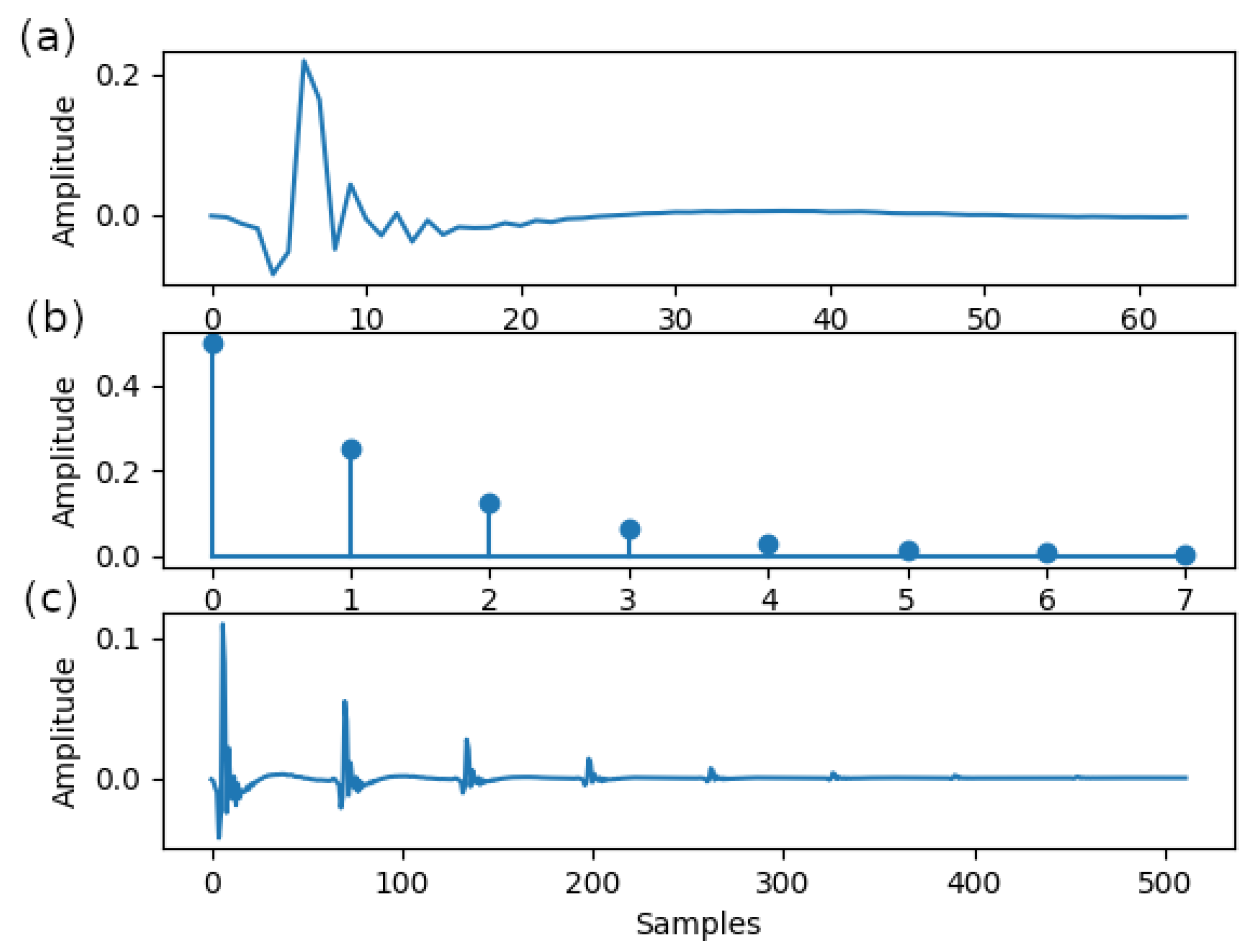
For the first set of simulations that implies the bilinear approach, we have considered the impulse responses depicted in Figure 6. In the first plot, Figure 6a, the first impulse response ${\mathbf{h}}_1$ from the G168 Recommendation [22] is represented (i.e., a 64 coefficients cluster). Next, Figure 6b depicts the second impulse response ${\mathbf{h}}_2$, evaluated as $h_{2l_2}={0.5}^{l2-1}$, with $l_2=1,2,\dots ,L_2$, where $L_2=8$. The third impulse response is the target that must be determined and is obtained as the Kronecker product between the first two impulse responses, i.e., $\mathbf{h}={\mathbf{h}}_2\otimes {\mathbf{h}}_1$. This impulse response is similar to the echo produced by an acoustic environment characterized by a reverberation effect and its length is $L=L_1{L}_2=512$ coefficients. Here, we consider the case of a linearly separable system, which is the benchmark of our approach, and show how it can be efficiently exploited in the framework of system identification problems. The impulse response from Figure 6c could correspond to a channel with echoes. This repetitive (but not periodic) structure could also result if a certain impulse response is followed by its reflections, e.g., as in wireless transmissions. The method allows temporal localization and magnitude estimation of the reflections, considering a temporal grid, without any restrictions of periodicity. However, the tensor-based adaptive algorithms can efficiently model the separable part of the system. The forgetting factor used for the RLS algorithm is computed as $\lambda =1-1/\left(KL\right)$, with $K=10$ in the bilinear context and $K=1$ in the trilinear context, while for the RLS-CKD algorithm is computed as ${\lambda }_i=1-1/\left(MK{L}_i\right)$, $i=1,2$, with $K=10$ and $M=1,3,5$.

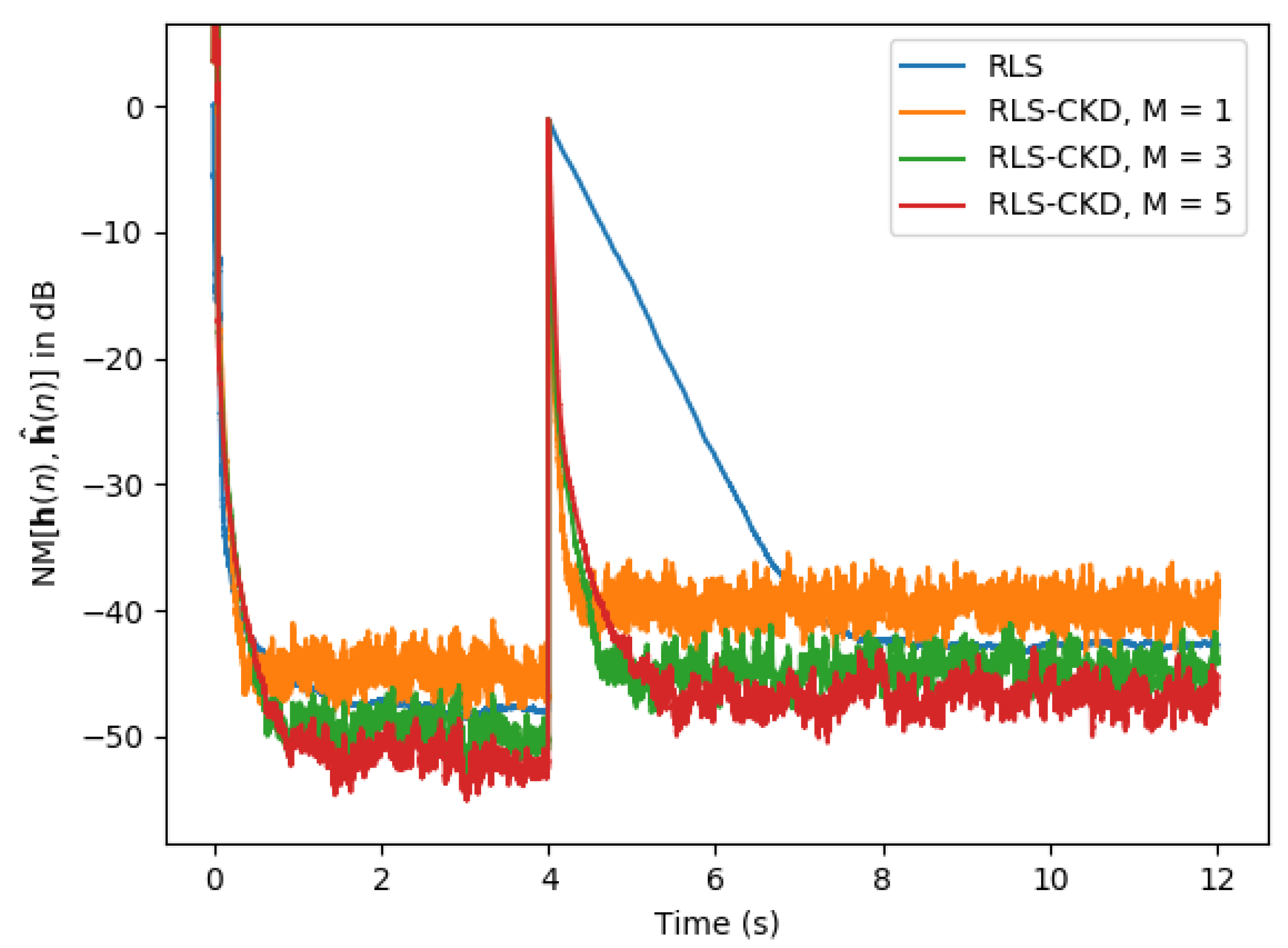
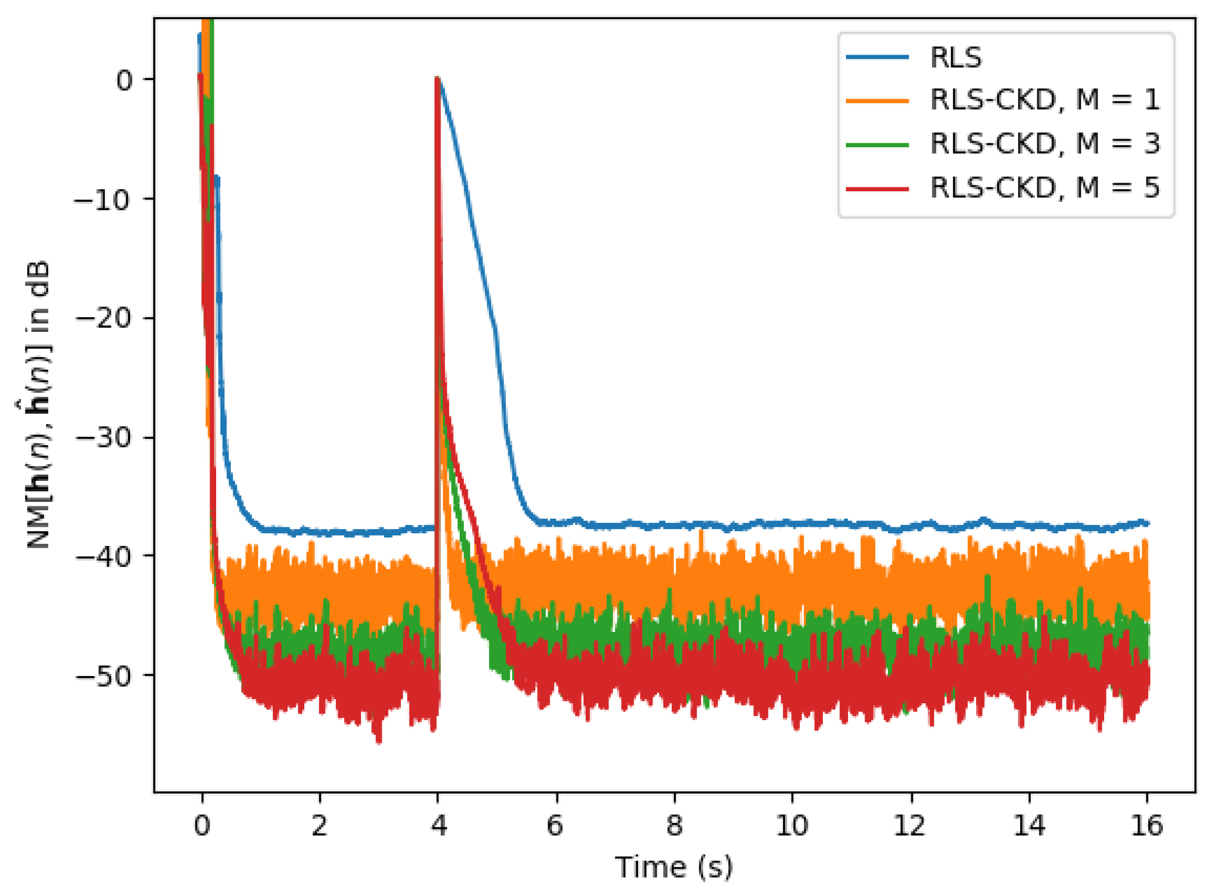
In the first simulation represented in Figure 7, we analyze the performance of the RLS-CKD algorithm with that of the classical RLS algorithm. The echo path changes after 4 s of simulation by changing the impulse response ${\mathbf{h}}_2$ with a random impulse response of the same length, with samples between 0 and 0.5. In the first part of the plot, we can remark that the RLS-CKD algorithm achieves a convergence rate similar to that of the classical RLS algorithm. Regarding the tracking capability, when the echo path changes, the RLS-CKD algorithm outperforms the RLS algorithm. The RLS-CKD achieves a normalized misalignment of −30 dB in less than 200 ms. We can remark that the constant value M only affects the normalized misalignment level when the echo path changes.

Next, in Figure 8, we analyze the behavior of the RLS-CKD algorithm in a scenario where the input signal is an AR(1) process. The echo path changes in the same manner as in the previous scenario. In this case, the RLS-CKD algorithm achieves an even lower normalized misalignment of almost 10 dB (e.g., when $M=5$) compared to the RLS algorithm. When the echo path changes, the values of M do not impact the RLC-CKD algorithm too much. This time, the RLS-CKD achieves a normalized misalignment of −40 dB in less than 500 ms, while the RLS algorithm requires at least 3 s to achieve a comparable level.

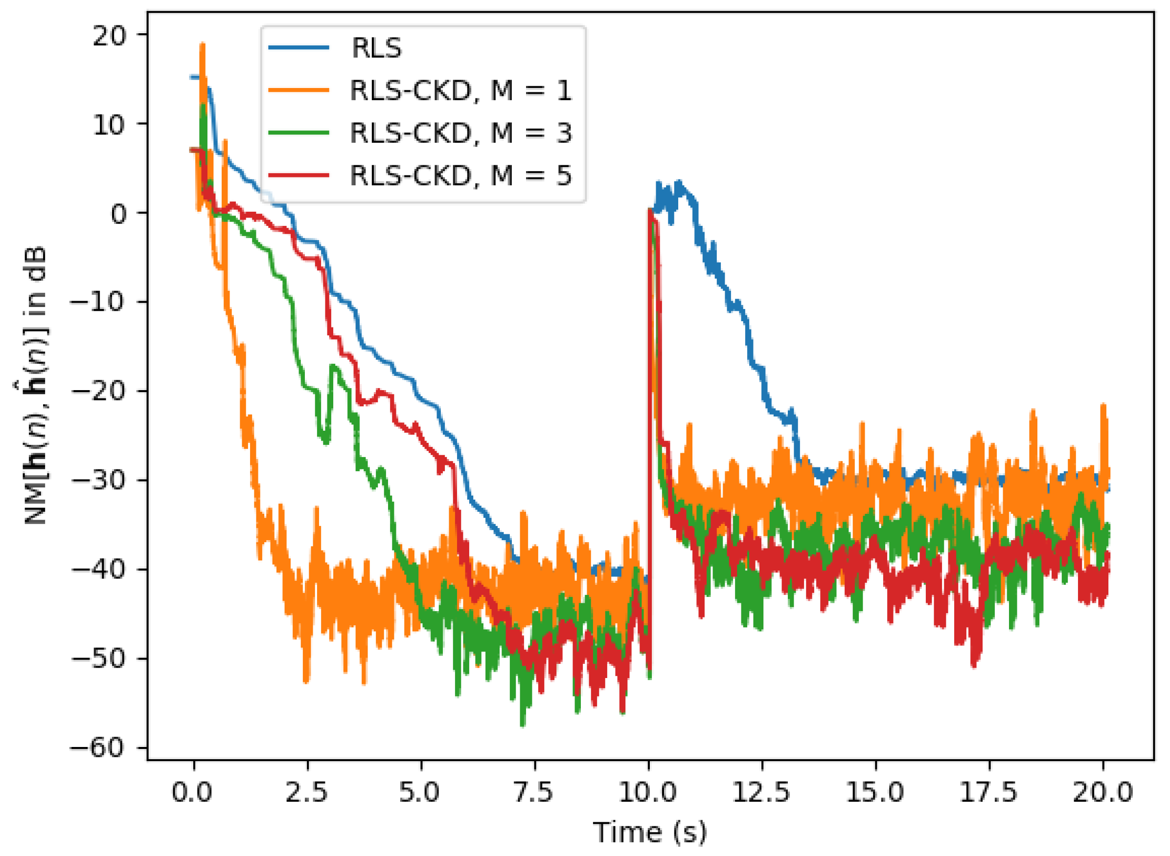
We conclude the first set of simulations with the scenario depicted in Figure 9, where the input signal is a speech sequence and the echo path changes in the middle of the simulation in the same manner.

As we can notice in Figure 9, the steady-state misalignment of the conventional RLS algorithm (the blue curve) is similar to the misalignment of the RLS-CKD algorithm using $M=1$, while the initial convergence rate and tracking of the proposed algorithm are much better. A larger value of M influences only the initial convergence rate of the RLS-CKD algorithm, but keeps the same fast tracking reaction. On the other hand, the steady-state misalignment of the RLS-CKD is improving for a larger value of M (i.e., for larger values of the forgetting factors ${\lambda }_i$, closer to 1).

Furthermore, we continue the simulations with the trilinear approach, based on the impulse responses from Figure 10. In this case, we have considered an even longer echo path of thousands of coefficients. The echo path of the system that must be identified is obtained as $\mathbf{h}={\mathbf{h}}_3\otimes {\mathbf{h}}_2\otimes {\mathbf{h}}_1$, of size $L=L_1{L}_2{L}_3=2048$, with ${\mathbf{h}}_1$ ($L_1=64$) from Figure 6a, ${\mathbf{h}}_2$ ($L_2=8$) from Figure 10a, and ${\mathbf{h}}_3$ ($L_3=4$) from Figure 10b. The second impulse response (i.e., ${\mathbf{h}}_2$) is randomly generated, with samples between 0 and 0.5, while the third impulse response (i.e., ${\mathbf{h}}_3$) is obtained as $h_{3l_3}={0.5}^{l3-1}$, with $l_3=1,2,\dots ,L_3$, where $L_3=4$.

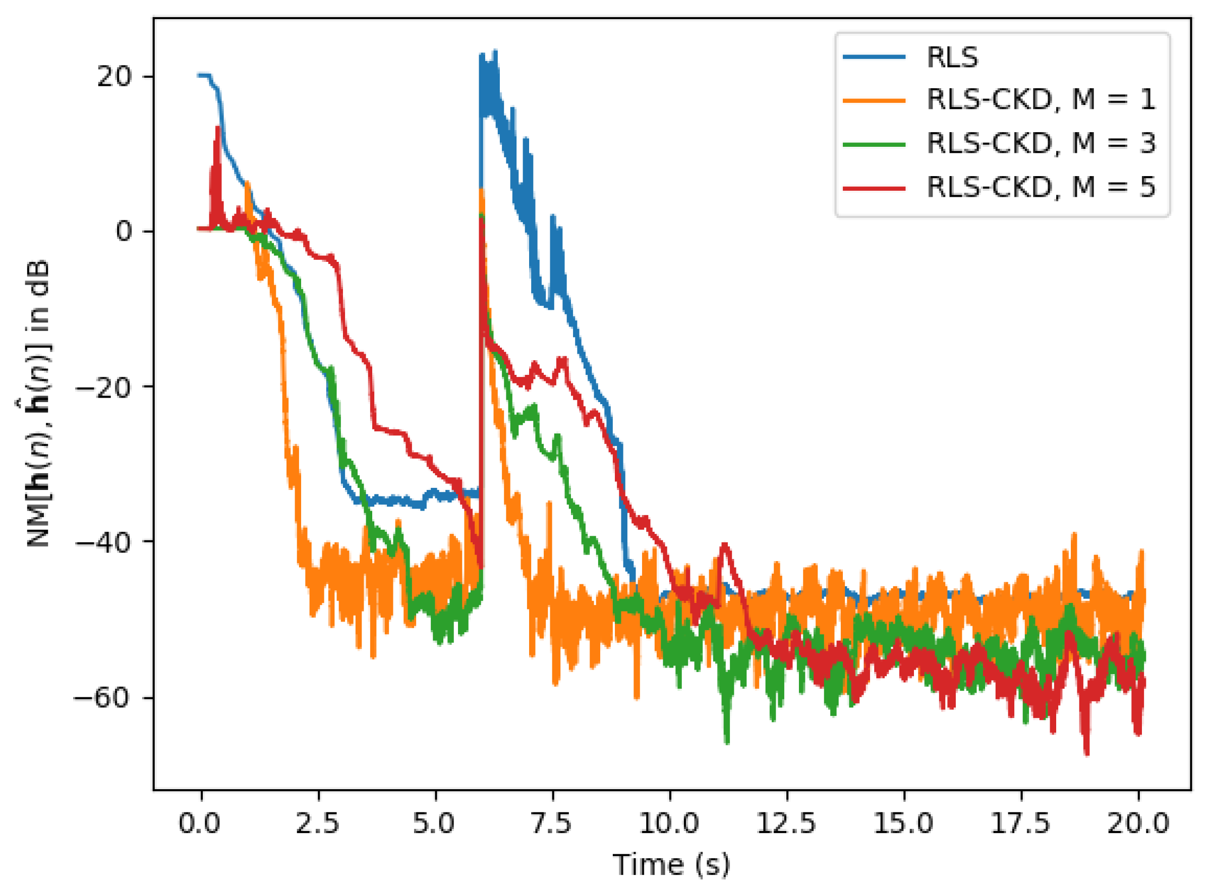
In Figure 11, the first simulation in the trilinear scenario is represented. The input signal is a white Gaussian noise and the echo path changes by generating ${\mathbf{h}}_3$ as a random impulse response after 4 s, so this impacts the whole system. It is worth noting that the RLS-CKD algorithm presents a slightly faster converge rate compared to that of the RLS algorithm and a lower normalized misalignment for $M=5$ of at least 10 dB. In terms of tracking, the RLS-CKD algorithm succeeds in re-estimating the new echo path and we can see that the smaller the forgetting factor is (i.e., $M=1$), the faster the tracking.

In the scenario represented in Figure 12, the input signal is an AR(1) process and the echo path changes by regenerating ${\mathbf{h}}_3$ after 4 s. The RLS-CKD algorithm outperforms the classical RLS algorithm in terms of convergence rate, normalized misalignment, and tracking capability, with a much lower computational complexity. Finally, in Figure 13, we conclude the set of simulations with a scenario where the input signal is a speech sequence. Again, the echo path changes by regenerating ${\mathbf{h}}_3$ after 6 s of simulation. While the classical RLS algorithm requires more than 3 s to achieve a reasonable normalized misalignment level, the RLS-CKD algorithm succeeds at estimating the target system, presenting a good tracking capability even when the echo path changes. However, for a faster convergence rate, the RLS-CKD algorithm requires a much lower forgetting factor (e.g., $M=1$). Also, the steady-state misalignment of the conventional RLS algorithm (after the change of the system) is similar to the misalignment of the RLS-CKD algorithm using $M=1$.

6. Conclusions

In this paper, we have introduced various memoryless and memory structures described by a bilinear input-output relation. Based on this approach, we have obtained a SISO system from a MISO system, which is a cascade of shorter length filters. We then developed the multilinear RLS algorithm considering the Kronecker product decomposition and outlining the reduction in terms of computational complexity. Finally, we have presented a set of simulations as a comparison between the newly developed RLS-CKD algorithm and the classical RLS algorithm. Simulations proved that the RLS-CKD algorithm outperforms the classical RLS algorithm in terms of convergence rate, normalized misalignment, and tracking capability. We can conclude that the RLS-CKD algorithm is a good candidate for real-time applications, which implies long length impulse responses and systems characterized by reverberation.