Abstract
The recently proposed tensor-based recursive least-squares dichotomous coordinate descent algorithm, namely RLS-DCD-T, was designed for the identification of multilinear forms. In this context, a high-dimensional system identification problem can be efficiently addressed (gaining in terms of both performance and complexity), based on tensor decomposition and modeling. In this paper, following the framework of the RLS-DCD-T, we propose a regularized version of this algorithm, where the regularization terms are incorporated within the cost functions. Furthermore, the optimal regularization parameters are derived, aiming to attenuate the effects of the system noise. Simulation results support the performance features of the proposed algorithm, especially in terms of its robustness in noisy environments.
1. Introduction
Nowadays, tensor-based signal processing methods are employed in many important real-world applications [1]. Such techniques can provide efficient solutions for big data problems [2], machine learning field [3], and source separation applications [4]. Recently, the iterative version of the Wiener filter was proposed for the identification of multilinear forms [5], e.g., for high-dimensional system identification problems (with a large parameter space).
Among the most popular adaptive filters, the recursive least-squares (RLS) algorithm represents a notable choice [6,7]. This algorithm is well-known for its fast convergence rate, especially when processing correlated input signals, but also for its high computational complexity. Despite their prohibitive nature, in classical and tensor-based structures, the RLS methods outperform their popular counterparts, such as the affine projection algorithm (APA) [8] and the algorithms based on the least-mean-square (LMS) method [9,10,11,12,13,14,15], which have been preferred in real-world applications due to their low arithmetic requirements. However, due to the tensor-based approach, the RLS algorithms designed for the identification of bilinear and trilinear forms [16,17] have become computationally efficient, as compared to the conventional LMS solutions. Furthermore, the recently proposed tensor-based RLS algorithm (RLS-T) [5] is tailored for the identification of multilinear forms. Basically, the high-dimensional system identification problem can be solved by using a decomposition into lower-dimensional structures, tensorized together.
Another tensor-based efficient adaptive filter that employs the combination between the RLS algorithm and the dichotomous coordinate descent (DCD) iterations, namely RLS-DCD-T [18], has been recently released. This algorithm uses a tensorial decomposition for multilinear forms and it has proven to be a powerful solution for tensor-based least-squares adaptive systems with low-complexity [19,20]. The DCD portion of the algorithm exploits the nature of the corresponding correlation matrices and solves auxiliary systems of equations using only additions and bit-shifts, as an alternative to traditional matrix inversion methods. Motivated by the appealing performance of the RLS-DCD-T, we aim to improve its robustness in noisy environments and we develop a regularized version of this algorithm. We will propose a variable regularized version in order to mitigate effects associated with non-stationary environments.
The regularization parameters of the RLS-DCD-T algorithm are usually used in the initialization stage (in order to prevent numerical problems). However, their influence is practically annihilated in the steady-state due to the forgetting factors [6]. The idea of performing regularization for the entire run of the adaptive systems has been initially introduced with the classical RLS algorithm [21]. In order to attenuate the effects of the system noise, optimal expressions were derived for the regularization parameters, which are related to the signal-to-noise ratio (SNR). The methods have also been successfully applied on the RLS-NKP algorithm [22] and on the RLS algorithms designed for the identification of bilinear [16], respectively, trilinear [23] forms.
2. System Context
We consider N impulse response vectors of lengths , which can be combined to form a larger multiple-input/single-output (MISO) global system. The N vectors describe the same number of corresponding individual channels:
where the superscript denotes the transpose operation and denotes the filter weights. For the rest of the paper, i will be employed for denoting elements associated with the i-th channel. The real-valued output signal corresponding to the global system at discrete-time index n can be expressed as:
where the input signals from (2) can be aggregated to form the tensorial structure using the components . Consequently, the input-output structure in (2) can be expressed as a multilinear form using the mode-i product , explained in [24]:
If of the vectors are considered fixed, then represents a linear function of the remaining vector .
The expression in (3) will be further developed in order to obtain a more intuitive form. The vectors will be combined using the outer product ∘, which can be expressed for two vectors as [15,18]. A new tensor can be defined as:
which is constituted with the elements . Furthermore, the vectorization operation applied to (4) leads to:
where, for any two vectors, , with ⊗ denoting the Kronecker product. Consequently, the output signal in (2) can be written as:
where
with representing the frontal slices of .
We can employ the notation:
for the input vector of length L = and we can express the global impulse response of length as:
The problem associated with the presented model is to indirectly find , by generating estimates for its individual components , using the so-called reference signal, given by the expression:
where is a noise signal uncorrelated with the output [15,25]. Considering that an estimate of the global impulse response is provided at every time index n, the corresponding a priori error signal can be written as:
The non-stationary nature of requires a solution that is capable to update the estimate with respect to any changes that might affect the global unknown system. Such condition eliminates the Wiener filter [6] as a valid option. Moreover, the adaptive systems that can be implemented in order to estimate fail to provide satisfactory results when they are working with large adaptive filters (hundreds/thousands of coefficients). The limited convergence speeds reduce tracking capabilities, even when employing the RLS family of adaptive methods, which are designed to mitigate the correlation of the input signals better than the classical workhorse of the industry (i.e., the LMS family of adaptive systems).
In [18,26], the nature of the described MISO systems was exploited by splitting the problem of identifying into multiple smaller problems, which target the separate estimation of the systems. The tracking capabilities proved to be drastically improved using considerable less arithmetic effort, with respect to the classical one-filter configurations. Moreover, the RLS-based adaptive algorithms combined with the DCD iterations were employed, thus offering a numerically stable RLS version with more appealing properties in terms of required chip areas. Consequently, an important remaining development direction is to improve the proposed solution’s robustness in low SNR conditions.
3. Robust Tensor-Based RLS Adaptive Algorithms
Despite the tracking speed improvements brought by employing fast converging algorithms (such as the RLS-based ones) with the split approach described in the previous section, the robustness in scenarios with high interference level is still an important topic to be studied. We will describe the recently proposed combination between the RLS adaptive algorithm and the DCD iterations working within the tensor-based framework for the identification of MISO systems. Subsequently, we will propose a variable regularization method for the correlation matrices associated with the RLS algorithm, which will considerably slow (or even halt) the update process corresponding to the filter estimates , when high noise levels bias the reference signal.
3.1. Tensor-Based Recursive Least-Squares Dichotomous Coordinate Descent Algorithm (RLS-DCD-T)
For the estimated impulse responses of the channels we can define the corresponding a priori error signals:
where are the individual outputs of the N channels. We can employ the vector defined in (7) and (8) to write the individual inputs of the N channels as:
where denotes the identity matrix of size .
Consequently, the individual output signals can be expressed as:
Moreover, it can be demonstrated that [17,26].
When applying the RLS algorithm in order to estimate (of length L) the cost function can be written as:
with the forgetting factor . Considering that the MISO system can be split in concordance with the N channels, with the corresponding impulse responses of lengths , the cost function for each channel can be written as:
where are the individual forgetting factors. The minimization of every single cost function (17), with respect to , can be performed by considering the other components fixed. The optimization is applied for the remaining one. When processing (17), we use the correlation matrices of each i channel:
respectively, the cross-correlation vectors between and :
and we obtain the set of normal equations [6]:
We obtain the N update relations corresponding to the individual filters by solving Equation (20). The straightforward solution (and the most complex) is to directly compute the inverse matrices . However, even for filters with tens of coefficients, this approach would often require too many chip resources. The prohibitive nature of the obvious solution led to extensive research efforts, which tried to find the best compromise between complexity on one side, respectively, performance and numerical stability, on the other side. The solution provided by the matrix inversion lemma (a.k.a. Woodbury’s matrix identity) [6] was often used as a reference in recent literature (i.e., an acceptable step in the right direction) [16,22]. However, the method is still too costly for real-time implementations.
In recent literature [27,28], the combination between the RLS algorithm and the DCD iterations demonstrated good performance, with an arithmetic complexity proportional to the filter length. The method defines the residual vector:
which is based on the consideration that a solution was provided at time index for (20). Several notations are also introduced to track the modifications brought to other elements of (20) at consecutive time indexes [18]:
where is a matrix, and , respectively, , are -valued column vectors.
The proposed method avoids computing a direct solution for the normal set of equations by writing (20) as:
where are the solutions that will be estimated for each channel. Equation (25) can be modified to eliminate , respectively, , by using (22) and (23), then (21):
Consequently, the new filter coefficients are obtained by adding the solutions vectors to the filter estimates from the previous time index:
The updates for the filter estimates obtained from solving (25) are based on the filter coefficients from the previous time index. The approach is suitable for DCD iterations [27,29], which requires considerable less arithmetic resources (in comparison to the direct approaches) and also provides updated values for the residual vectors . By employing (23) and (24), then , in
we can write:
Using (30) and (31), the matrix and the vector will be replaced in (26), then with (21) and (13), we can write:
The last expression shows how the right side of (25) can be updated with minimum arithmetic effort, a task which is solved by the DCD portion of the algorithm. The overall RLS-DCD adaptive algorithm based on tensorial forms (also called RLS-DCD-T) is presented in Algorithm 1.
| Algorithm 1 Exponential Weighted RLS-T Algorithm for a single channel. |
| : |
| Set |
| 0 |
| 1 Compute , based on (14) |
| 2 |
| 3 |
| 4 |
| 5 |
| 6 |
| 7 |
It can be noticed that the problem of determining the filter estimates is split into firstly computing each of the N increment vectors independently, then adding them to the estimates obtained from the previous adaptive system iteration. In step 2 of the algorithm, the update of matrix requires shifting all its values with the exception of the first column and the first row – both have the same set of values, which have to be updated [18,28]. The notation represents the first value of the vector . Moreover, step 6 shows that the residual vectors are generated by the DCD method and they will be used at the next time index to generate the right side of the auxiliary sets of normal equations, which will again be processed by the DCD iterations.
In Algorithm 2 the DCD method with a is presented. It works using a approach and it performs (for each channel) comparisons between the main diagonal of correlation matrix and the residual vector (equivalent positions) in order to determine at which indexes to perform modifications for the vector . The corresponding value updates are equivalent to bits set to ’1’ for the estimated coefficients situated on various positions in the solution vector. In software validations, such operations are simulated using the step size and the maximum expected amplitude of the solution values H, which is initialized using a power of two. The values in and are expected to be in the interval .
| Algorithm 2 The DCD iterations with a leading element. |
| The content of the table is correct. |
| 1 |
| 2 && |
| 3 |
| 4 |
| 5 |
The entire DCD process (i.e., search for the maximum value, verify conditions, update values and indexes) requires only additions and bit-shifts, which makes it an attractive choice for hardware implementations. The maximum number of updates for any given RLS-DCD-T iteration is denoted in Algorithm 2 with (for channel i). The approach presented in Algorithm 1 demonstrated in the past, for relatively low values of , performance comparable to the classical RLS algorithm. Excepting step 1, the overall complexity associated with the RLS-DCD-T is a sum of values approximately proportional to the individual filter lengths. More information about the RLS-DCD versions can be found in [18,22,27,28] and in corresponding references.
3.2. Robust RLS-DCD-T Adaptive Algorithm Based on Matrix Regularization
In this sub-section we concentrate on enhancing the robustness of the RLS-DCD-T algorithm by focusing on the regularization parameter for each of the N channels. Its usual value is a constant which traditionally influences the first iterations of the adaptive system in order to mitigate the ill-conditioned nature of the correlation matrices . Our purpose is to change the scope of this parameter in order to have more significance in practice. By adjusting it in real-time, we aim to improve the performance of the RLS-DCD-T in low SNR conditions, when the reference signal is affected by an undesired additive noise.
We reconsider the least-squares criterion in order to include for the entire run of the algorithm the presence of the regularization parameter. Therefore, the individual cost functions will be rewritten as:
where denotes the norm. The update equation for each filter can accordingly be expressed as:
The contribution described in (38) is strongly connected to and comprises the effects of the interference that we aim to mitigate. The expression for represents the solution for the system of equations:
Correspondingly, for each channel, we can define another error signal for the newly introduced system, as a difference between the reference signal and the output of the filter updates in (38):
For the new structure we can define the goal of recovering/estimating the noise signal and we will find an expression for in order to have equality between the expected value of and the variance of the noise signal :
We will develop (41) by squaring it and applying the expectation operator on both sides of the equal sign. With this purpose, a few approximations will be explained, then used in the resulting computations. Firstly, for a large enough time index n (i.e., the RLS-DCD-T has functioned for a sufficient amount of time), the matrices defined in (18) can be written as:
For the previous expression we need to examine the value of the expectation operator. We start by using (14), then the transpose and the mixed-product properties of the Kronecker product. Only for this portion of the algorithm, we also consider to be uncorrelated with , respectively, that are approximately diagonal matrices, so that , where is the variance of . Thus, we obtain:
Considering that we can approximate we reach the expression:
We also consider that the forgetting factors can be approximately chosen having the values , and together with (46), they can be used to rewrite (43) as
where
Moreover, we can express:
and proceed to squaring, respectively, applying the expectation operator on (41). We replace by using (38), and after some computations we find:
where denotes the variance of .
We can divide (50) by and write a squared binomial on the right side of the equal, then use:
respectively,
Finally, after a few more calculations, we reach a second degree equation:
where we consider as the unknown variable. From this equation we take into consideration only the positive solution:
3.3. Practical Considerations
From a practical point of view, once has been determined with (54), it is valid as long as the unknown systems comprising the MISO model remain the same and the statistical properties of the corresponding signals are unchanged. However, the practical applications associated with such presumptions are extremely limited. Consequently, we will adjust the proposed model in order to perform real-time estimations for all involved parameters.
Firstly, the variances , and have to be estimated at every time index n. We consider that the adaptive algorithm has converged to a certain degree and we will use , as the value for is not directly available. We will employ the exponential window function:
where determines the memory of the window, respectively, represents in turn the signals , , and .
Secondly, working with the same assumption that the adaptive system has converged to a certain point, an estimate for the SNR can be determined based on (51), respectively, (52), for each channel as:
Considering the above arguments, which proved correct when applied to other adaptive systems with variable parameters [16,22,30], the computation of becomes straightforward for each channel. The values of are used in the DCD portion of the RLS-DCD-T method in order to adjust the main diagonal of in the desired direction. More precisely, when the value of increases, the comparisons performed in the DCD will reduce the number of filter updates—this is desirable in high interference scenarios. On the other hand, in high SNR situations, the successful updates should be performed as in Algorithm 1 for , due to the negligible influence of .
With a small cost in arithmetic complexity, the algorithm gains much needed robustness. Moreover, it is expected to work properly in tracking scenarios, when one or more of the smaller unknown systems change. We call the new algorithm the variable regularized RLS-DCD-T algorithm, namely VR-RLS-DCD-T, which is summarized in Algorithm 3. It can be noticed in steps 5 a) to 5 d) that the extra computational requirements of the VR-RLS-DCD-T consist mostly of multiplications and additions. The overall arithmetic effort of the update process remains a sum of values proportional to each of the filter lengths. Two extra divisions and one square root operation have to be performed for each channel. From a practical point of view, when implementations are performed on Field Programmable Gate Array (FPGA) devices, a single Digital Signal Processing (DSP) block can be employed functioning in two distinct arithmetic modes.
| Algorithm 3 VR-RLS-DCD-T. |
| : |
| Set |
| 0 |
| 1 Compute , based on (14) |
| 2 |
| 3 |
| 4 |
| 5 a) for and |
| 5 b) |
| 5 c) |
| 5 d) |
| 6 |
| 7 |
4. Simulation Results
Several configurations are simulated in order to validate the performance of the proposed algorithm in scenarios with low SNR conditions. We also verify that the VR-RLS-DCD-T works well in tracking situations, when the unknown global system changes suddenly. We generate such a modification after the convergence is achieved, by altering the sign of one of the constituent systems, which are combined using the model described in (9). The experiments work with , respectively, , smaller systems of lengths (depending on the case). The presented scenarios aim to demonstrate the tracking capabilities and the robustness of the proposed VR-RLS-DCD-T, with respect to the already studied RLS-T [17], respectively, RLS-DCD-T [18], which perform identification of the smaller impulse responses . For the tracking situations we also use as reference the classical RLS method based on Woodburry’s identity for the direct identification of [6].
Two of the smaller systems [, ] are comprised of samples taken from the impulse responses in the G.168 ITU-T Recommendation [31] – vectors with , respectively, , values. The other two systems systems [, ] are obtained using the functions , respectively, , with and . We use as input signals Gaussian sequences filtered through an auto-regressive AR(1) system with the pole 0.85, in order to have highly correlated input samples. For the output of the unknown global system , the reference signal has an experimental SNR ratio set to 15 dB. In the intervals with low SNR conditions, the corresponding value is modified to −15 dB.
The forgetting factors for the adaptive filters are chosen as for the tensor-based methods, respectively, as for the classical RLS. The forms facilitate efficient hardware implementations of multiplications [20,32]. For a similar reason, the filter lengths have the form , respectively, . Furthermore, for the specific parameters of the DCD iterations, the maximum expected amplitudes of the filter coefficients are set to , with the representation bits. In accordance with our team’s previously published or several referenced studies, the maximum number of allowed updates for each filter is set to [18,20,22,28].
In order to measure the accuracy of the unknown global system identification, we employ the normalized misalignment , where the global filter estimate is reconstituted using the smaller N filter estimates . The tensor-based adaptive filters are initialized using the method recommended in [15] and the initial convergence is not shown, as it is not considered relevant [33].
The first experiment was performed for a tracking scenario with coefficients for , which can be decomposed in three smaller systems with lengths and . The global impulse response suffers a sudden change and all adaptive methods must go through a re-convergence process. The decomposition based algorithms use the same set of forgetting factors, respectively, the value of for the RLS method was chosen to match the performance of the tensor-based algorithms at convergence state. It can be noticed in Figure 1 that the tensor-based methods benefit from the split structure working with smaller adaptive filters and converge considerably faster than the RLS method after the sudden change in the global system. Moreover, it is important to notice that the VR-RLS-DCD-T offers tracking performance similar with the RLS-DCD-T and the RLS-T.
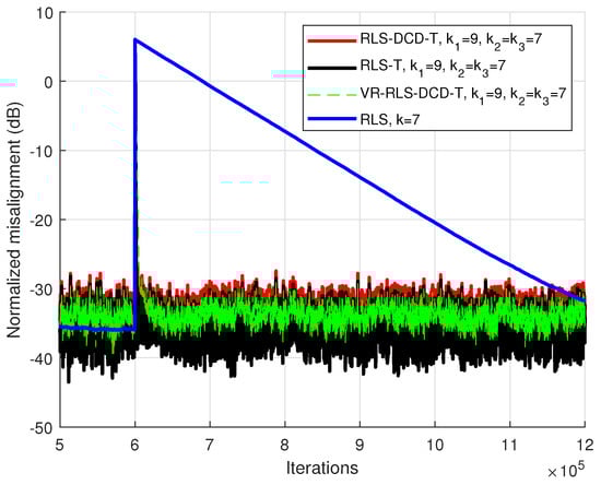
Figure 1.
Performance of the RLS-DCD-T, RLS-T, VR-RLS-DCD-T and RLS algorithms, for the identification of the global impulse response in a tracking scenario. The tensor-based filters have and . The input signal is an AR(1) sequence with the pole 0.85, , and .
In Figure 2, the same algorithms were simulated in the same type of scenario (i.e., a tracking situation) with a different configuration. The global system has the length , with a decomposition performed with 4 smaller impulse responses having , , respectively, . Similar conclusions apply regarding the tracking capabilities when the global system is changed. The tensor-based variants show considerably better performance than the RLS. Moreover, the RLS-DCD-T and the VR-RLS-DCD-T methods manage to perform in the same manner as the RLS-T adaptive algorithm, while requiring lesser computational resources for the coefficients update process.
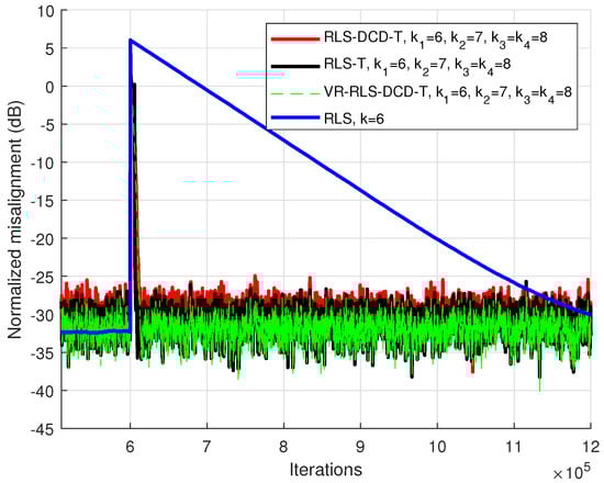
Figure 2.
Performance of the RLS-DCD-T, RLS-T, VR-RLS-DCD-T and RLS algorithms, for the identification of the global impulse response in a tracking scenario. The tensor-based filters have , and . The input signal is an AR(1) sequence with the pole 0.85, , and .
It is obvious that the direct approach of estimating leads to an unwanted compromise between tracking speed and accuracy. If the same performance is targeted at convergence state, the RLS would be outperformed in any situation where going through the converging process is necessary. The conclusion includes the case when the filter coefficients are temporarily biased by low SNR conditions. On the other hand, if the tracking speed is matched between the RLS method and its tensor-based counterparts (by using for the former a smaller value of ), the accuracy of the estimation is reduced at steady-state. Consequently, the next scenarios will only compare the tensor-based algorithms and show the improved robustness of the proposed VR-RLS-DCD-T for several configurations associated with the presented MISO model.
The global systems from the first two scenarios were employed for another validation type. In Figure 3 and Figure 4, for a duration of 10,000 samples, the SNR value is temporarily set to −15 dB. It can be noticed that the RLS-T and the RLS-DCD-T are strongly affected by the alteration of the reference signals. However, the change in conditions has diminished effects on the VR-RLS-DCD-T adaptive system. When the undesired phenomenon halts, the corresponding recovery process requires less iterations to return to the previous state.
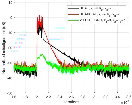
Figure 3.
Performance of the RLS-T, RLS-DCD-T, and VR-RLS-DCD-T, for the identification of the global impulse response . The SNR drops to −15 dB for 10,000 iterations. The tensor-based filters have and . The input signal is an AR(1) sequence with the pole 0.85, , and .
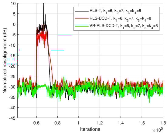
Figure 4.
Performance of the RLS-T, RLS-DCD-T, and VR-RLS-DCD-T, for the identification of the global impulse response . The SNR drops to −15 dB for 10,000 iterations. The tensor-based filters have , , and . The input signal is an AR(1) sequence with the pole 0.85, , and .
The robustness validation was also performed for a third (and even longer) global system with coefficients, which is decomposed using four impulse responses with equal lengths . The results are illustrated in Figure 5. It is clear that the VR-RLS-DCD-T outperforms the other tensor-based algorithms and has the least affected filter coefficients during the high interference period. The tensor-based NLMS algorithm [11] was also tested for this scenario and the results were added in Figure 5. For one of the NLMS-T versions, the step-size was chosen to generate similar convergence with the RLS-based methods at steady-state. However, the recovery process requires the largest number of iterations, with respect to the RLS-based counterparts. Moreover, it can be noticed that attempting to match the convergence speed of the NLMS-T with the RLS-T versions (by using a larger ) leads to lower accuracy at steady-state.
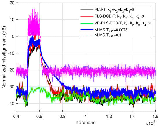
Figure 5.
Performance of the RLS-T, RLS-DCD-T, VR-RLS-DCD-T, and the NLMS-T, for the identification of the global impulse response . The SNR drops to −15 dB for 10,000 iterations. The tensor-based filters have . The input signal is an AR(1) sequence with the pole 0.85, , and .
5. Conclusions
This paper proposed a robust low-complexity RLS adaptive algorithm, which is designed on tensor-based decomposition and employs the DCD iterations to solve the set of normal equations specific to the RLS methods. The algorithm benefits from the reduced arithmetic requirements provided by splitting one major system identification problem into several smaller corresponding problems. Moreover, the DCD iterations require only bit-shifts and additions, which makes it attractive for practical applications. The VR-RLS-DCD-T has minimal additions to the arithmetic complexity and is designed for improved robustness in low SNR conditions, by influencing the update process through a continuous regularization process of the corresponding correlation matrices.
Simulations were performed in order to validate the proposed method in two types of scenarios. Firstly, we demonstrated that the tracking capabilities remain similar with other RLS tensor-based adaptive systems. Secondly, validations were completed with high noise levels affecting the reference signals. The results showed a robust behaviour in low SNR scenarios, when the VR-RLS-DCD-T filter coefficients suffer minimal modifications, which allow for minimal re-convergence periods after the interference signals cease.
In perspective, we aim to even further develop variable regularized RLS-DCD-T methods by introducing a version based on sliding windows [33]. Moreover, fixed-point FPGA implementations will be performed for MISO configurations as the next step towards our final goal of providing a better alternative for current practical applications.
Author Contributions
Conceptualization, C.-L.S. and C.E.-I.; Formal Analysis, C.A.; Methodology, C.-L.S. and C.E.-I.; Software, I.-D.F. and C.-L.S. All authors have read and agreed to the published version of the manuscript.
Funding
This work was supported by a grant of the Romanian Ministry of Education and Research, CNCS–UEFISCDI, project number PN-III-P1-1.1-TE-2019-0529, within PNCDI III.
Data Availability Statement
The data presented in this study are available on request from the corresponding author.
Conflicts of Interest
The authors declare no conflict of interest.
References
- Cichocki, A.; Mandic, D.; De Lathauwer, L.; Zhou, G.; Zhao, Q.; Caiafa, C.; PHAN, H.A. Tensor Decompositions for Signal Processing Applications: From two-way to multiway component analysis. IEEE Signal Process. Mag. 2015, 32, 145–163. [Google Scholar] [CrossRef] [Green Version]
- Vervliet, N.; Debals, O.; Sorber, L.; De Lathauwer, L. Breaking the Curse of Dimensionality Using Decompositions of Incomplete Tensors: Tensor-based scientific computing in big data analysis. IEEE Signal Process. Mag. 2014, 31, 71–79. [Google Scholar] [CrossRef]
- Sidiropoulos, N.D.; De Lathauwer, L.; Fu, X.; Huang, K.; Papalexakis, E.E.; Faloutsos, C. Tensor Decomposition for Signal Processing and Machine Learning. IEEE Trans. Signal Process. 2017, 65, 3551–3582. [Google Scholar] [CrossRef]
- Boussé, M.; Debals, O.; De Lathauwer, L. A Tensor-Based Method for Large-Scale Blind Source Separation Using Segmentation. IEEE Trans. Signal Process. 2017, 65, 346–358. [Google Scholar] [CrossRef]
- Dogariu, L.M.; Ciochină, S.; Paleologu, C.; Benesty, J.; Oprea, C. An Iterative Wiener Filter for the Identification of Multilinear Forms. In Proceedings of the 2020 43rd International Conference on Telecommunications and Signal Processing (TSP), Milan, Italy, 7–9 July 2020; pp. 193–197. [Google Scholar] [CrossRef]
- Haykin, S. Adaptive Filter Theory, 4th ed.; Prentice Hall: Upper Saddle River, NJ, USA, 2002. [Google Scholar]
- Benesty, J.; Huang, Y. Adaptive Signal Processing–Applications to Real-World Problems; Springer: Berlin/Heidelberg, Germany, 2003. [Google Scholar]
- Dogariu, L.M.; Elisei-Iliescu, C.; Paleologu, C.; Benesty, J.; Ciochină, S. A Tensorial Affine Projection Algorithm. In Proceedings of the 2021 International Symposium on Signals, Circuits and Systems (ISSCS), Iasi, Romania, 15–16 July 2021; pp. 1–4. [Google Scholar] [CrossRef]
- Rupp, M.; Schwarz, S. A tensor LMS algorithm. In Proceedings of the 2015 IEEE International Conference on Acoustics, Speech and Signal Processing (ICASSP), South Brisbane, Australia, 19–24 April 2015; pp. 3347–3351. [Google Scholar] [CrossRef]
- Rupp, M.; Schwarz, S. Gradient-based approaches to learn tensor products. In Proceedings of the 2015 23rd European Signal Processing Conference (EUSIPCO), Nice, France, 31 August–4 September 2015; pp. 2486–2490. [Google Scholar]
- Dogariu, L.M.; Paleologu, C.; Benesty, J.; Oprea, C.; Ciochină, S. LMS Algorithms for Multilinear Forms. In Proceedings of the 2020 International Symposium on Electronics and Telecommunications (ISETC), Timisoara, Romania, 5–6 November 2020; pp. 1–4. [Google Scholar] [CrossRef]
- Kuhn, E.V.; Pitz, C.A.; Matsuo, M.V.; Bakri, K.J.; Seara, R.; Benesty, J. A Kronecker product CLMS algorithm for adaptive beamforming. Digit. Signal Process. 2021, 111, 102968. [Google Scholar] [CrossRef]
- Fîciu, I.D.; Stanciu, C.; Anghel, C.; Paleologu, C.; Stanciu, L. Combinations of Adaptive Filters within the Multilinear Forms. In Proceedings of the 2021 International Symposium on Signals, Circuits and Systems (ISSCS), Iasi, Romania, 15–16 July 2021; pp. 1–4. [Google Scholar] [CrossRef]
- Bakri, K.J.; Kuhn, E.V.; Seara, R.; Benesty, J.; Paleologu, C.; Ciochină, S. On the stochastic modeling of the LMS algorithm operating with bilinear forms. Digit. Signal Process. 2022, 122, 103359. [Google Scholar] [CrossRef]
- Dogariu, L.M.; Stanciu, C.L.; Elisei-Iliescu, C.; Paleologu, C.; Benesty, J.; Ciochină, S. Tensor-Based Adaptive Filtering Algorithms. Symmetry 2021, 13, 481. [Google Scholar] [CrossRef]
- Elisei-Iliescu, C.; Stanciu, C.; Paleologu, C.; Benesty, J.; Anghel, C.; Ciochină, S. Efficient recursive least-squares algorithms for the identification of bilinear forms. Digit. Signal Process. 2018, 83, 280–296. [Google Scholar] [CrossRef]
- Elisei-Iliescu, C.; Dogariu, L.M.; Paleologu, C.; Benesty, J.; Enescu, A.A.; Ciochină, S. A Recursive Least-Squares Algorithm for the Identification of Trilinear Forms. Algorithms 2020, 13, 135. [Google Scholar] [CrossRef]
- Fîciu, I.D.; Stanciu, C.L.; Anghel, C.; Elisei-Iliescu, C. Low-Complexity Recursive Least-Squares Adaptive Algorithm Based on Tensorial Forms. Appl. Sci. 2021, 11, 8656. [Google Scholar] [CrossRef]
- Stanciu, C.; Ciochină, S. A robust dual-path DCD-RLS algorithm for stereophonic acoustic echo cancellation. In Proceedings of the International Symposium on Signals, Circuits and Systems ISSCS2013, Iasi, Romania, 11–12 July 2013; pp. 1–4. [Google Scholar] [CrossRef]
- Stanciu, C.; Anghel, C. Numerical properties of the DCD-RLS algorithm for stereo acoustic echo cancellation. In Proceedings of the 2014 10th International Conference on Communications (COMM), Bucharest, Romania, 29–31 May 2014; pp. 1–4. [Google Scholar] [CrossRef]
- Benesty, J.; Paleologu, C.; Ciochina, S. Regularization of the RLS Algorithm. IEICE Trans. 2011, 94-A, 1628–1629. [Google Scholar] [CrossRef]
- Elisei-Iliescu, C.; Paleologu, C.; Benesty, J.; Stanciu, C.; Anghel, C.; Ciochină, S. Recursive Least-Squares Algorithms for the Identification of Low-Rank Systems. IEEE/Acm Trans. Audio Speech Lang. Process. 2019, 27, 903–918. [Google Scholar] [CrossRef]
- Elisei-Iliescu, C.; Paleologu, C.; Benesty, J.; Stanciu, C.; Anghel, C. A Regularized RLS Algorithm for the Identification of Third-Order Tensors. In Proceedings of the 2020 International Symposium on Electronics and Telecommunications (ISETC), Timisoara, Romania, 5–6 November 2020; pp. 1–4. [Google Scholar] [CrossRef]
- Andrzej, C.; Rafal, Z.; Anh Huy, P.; Shun-ichi, A. Nonnegative Matrix and Tensor Factorizations: Applications to Exploratory Multi-Way Data Analysis and Blind Source Separation; John Wiley and Sons, Ltd.: Hoboken, NJ, USA, 2009. [Google Scholar]
- Dogariu, L.M.; Paleologu, C.; Benesty, J.; Stanciu, C.L.; Oprea, C.C.; Ciochină, S. A Kalman Filter for Multilinear Forms and Its Connection with Tensorial Adaptive Filters. Sensors 2021, 21, 3555. [Google Scholar] [CrossRef] [PubMed]
- Dogariu, L.M.; Ciochină, S.; Benesty, J.; Paleologu, C. System Identification Based on Tensor Decompositions: A Trilinear Approach. Symmetry 2019, 11, 556. [Google Scholar] [CrossRef] [Green Version]
- Zakharov, Y.V.; White, G.P.; Liu, J. Low-Complexity RLS Algorithms Using Dichotomous Coordinate Descent Iterations. IEEE Trans. Signal Process. 2008, 56, 3150–3161. [Google Scholar] [CrossRef] [Green Version]
- Stanciu, C.; Benesty, J.; Paleologu, C.; Gänsler, T.; Ciochină, S. A widely linear model for stereophonic acoustic echo cancellation. Signal Process. 2013, 93, 511–516. [Google Scholar] [CrossRef]
- Liu, J.; Zakharov, Y.V.; Weaver, B. Architecture and FPGA Design of Dichotomous Coordinate Descent Algorithms. IEEE Trans. Circuits Syst. I: Regul. Pap. 2009, 56, 2425–2438. [Google Scholar] [CrossRef]
- Elisei-Iliescu, C.; Stanciu, C.; Paleologu, C.; Benesty, J.; Anghel, C.; Ciochină, S. Robust variable-regularized RLS algorithms. In Proceedings of the 2017 Hands-free Speech Communications and Microphone Arrays (HSCMA), San Francisco, CA, USA, 1–3 March 2017; pp. 171–175. [Google Scholar] [CrossRef]
- Digital Network Echo Cancellers; ITU-T Recommendations G.168. Available online: https://www.itu.int/rec/T-REC-G.168/en (accessed on 21 August 2021).
- Stanciu, C.; Anghel, C.; Stanciu, L. Efficient FPGA implementation of the DCD-RLS algorithm for stereo acoustic echo cancellation. In Proceedings of the 2015 International Symposium on Signals, Circuits and Systems (ISSCS), Iasi, Romania, 9–10 July 2015; pp. 1–4. [Google Scholar] [CrossRef]
- Zakharov, Y.V.; Nascimento, V.H. DCD-RLS Adaptive Filters With Penalties for Sparse Identification. IEEE Trans. Signal Process. 2013, 61, 3198–3213. [Google Scholar] [CrossRef]
Publisher’s Note: MDPI stays neutral with regard to jurisdictional claims in published maps and institutional affiliations. |
© 2022 by the authors. Licensee MDPI, Basel, Switzerland. This article is an open access article distributed under the terms and conditions of the Creative Commons Attribution (CC BY) license (https://creativecommons.org/licenses/by/4.0/).