Multivariate Demand Forecasting for Rental Bike Systems Based on an Unobserved Component Model

Abstract

Many German cities, municipalities and transport associations are expanding their bike-sharing systems (BSS) to offer citizens a cost-effective and climate-friendly means of transport and an alternative to private motorized transport (PMT). However, operators face the challenge of generating high-quality predictive analyses and time series forecasts. In particular, the prediction of demand is a key component to foster data-driven decisions. To address this problem, an Unobserved Component Model (UCM) has been developed to predict the monthly rentals of a BSS, whereby the station-based BSS VRNnextbike, including over 2000 bikes, 297 stations and 21 municipalities, is employed as an example. The model decomposes the time series into trend, seasonal, cyclical, auto-regressive and irregular components for statistical modeling. Additionally, the model includes exogenous factors such as weather, user behavior (e.g., traveled distance), school holidays and COVID-19 relevant covariates as independent effects to calculate scenario based forecasts. It can be shown that the UCM calculates reasonably accurate forecasts and outperforms classical time series models such as ARIMA(X) or SARIMA(X). Improvements were observed in model quality in terms of AIC/BIC (2.5% to 22%) and a reduction in error metrics from 15% to 45% depending on the considered model.

1. Introduction

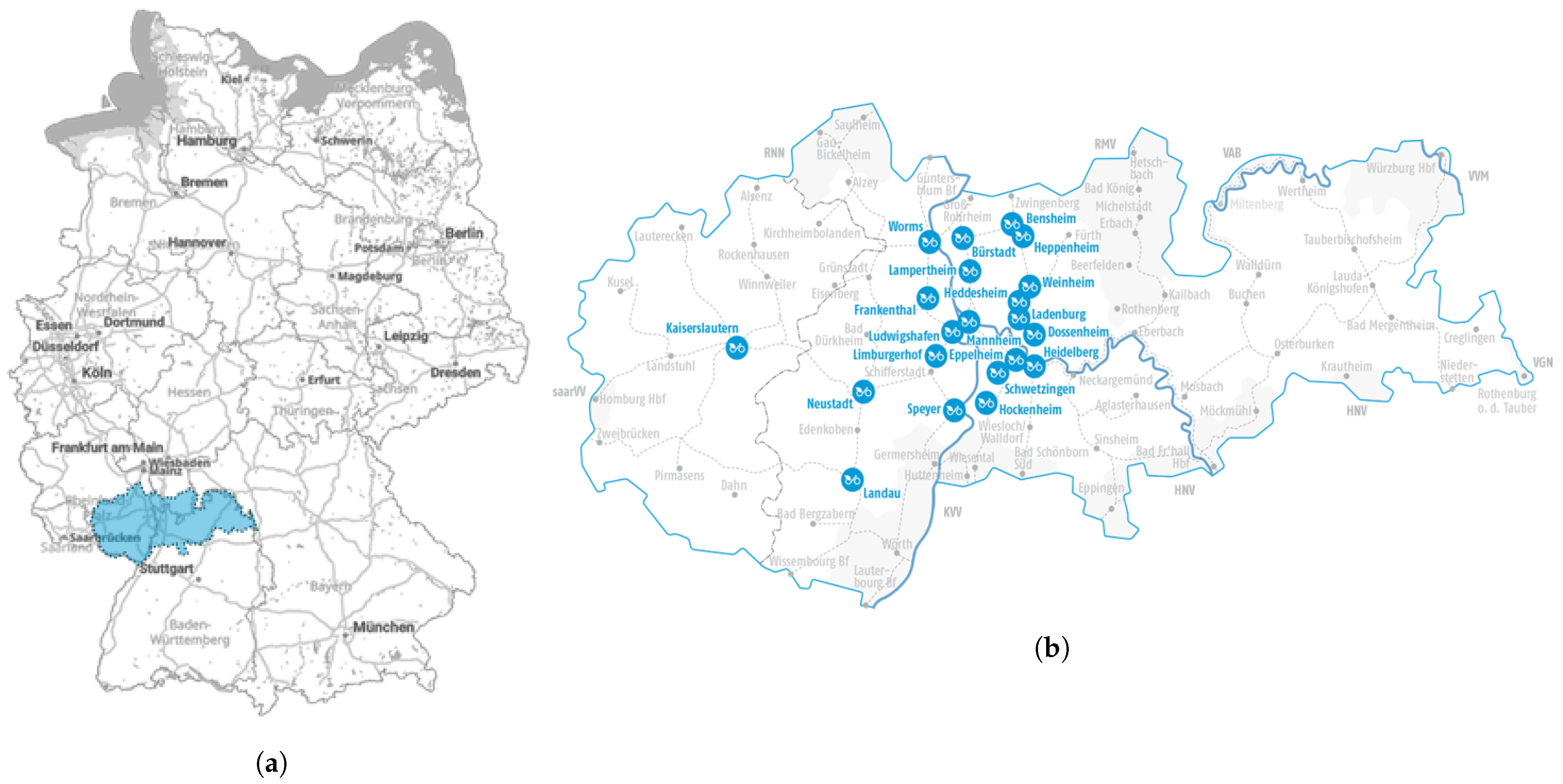
In recent years more and more bike sharing systems (BSS) have been established in German cities and urban areas. BBS offer commuters, residents and tourists an environmentally friendly and cost-effective transport service. BSSs are operated by municipalities, companies, and transport associations. The latter also includes the transport association Rhine-Neckar (VRN), which has operated a BSS called VRNnextbike since 2012. Currently, the bike service is offered in 21 locations, including four major cities (Mannheim, Ludwigshafen, Heidelberg, Kaiserslautern), 16 minor cities and five smaller towns. These municipalities form a supply region (Figure 1), which includes over 2000 bikes and 297 stations in total.

With the increasing growth of the BSS market, it is becoming particularly important for operators to predict and analyze the demand of rentals. The development of rentals is a relevant factor for BSSs and therefore the forecast of this parameter is a key component for making strategic and executive decisions. Operators, however, face the challenge of generating long-term forecasts. Another problem is that the data pool is growing rapidly and the data sets need to be updated and maintained. Conversely, this means that the models must be fitted repeatedly to the new data in order to improve performance and to be able to model new trends and effects.

With the use of predictive analytics, future developments can be predicted based on historical data. Such forecast models can be grouped into several categories, including statistical methods such as traditional time series models like ARIMA (Auto-Regressive Integrated Moving Average) [1], machine learning methods such as artificial neural networks (ANNs) [2] or Gradient Tree Boosting systems (AdaBoost, XGBoost) [3,4] and deep learning methods such as Long Short-Term Memories (LSTMs) [5] or Temporal Convolutional Networks (TCNs) [6]. The specific methods and models are all applicable for time series forecasts (TSF) but perform differently for short-term (STSF) or long-term forecasts (LTSF). The research focus has been mainly on machine learning models, station-based or short-term approaches in recent years [7,8,9]. For this reason, other models should also be included in the current research in the field of BSS demand forecasting. Another alternative could be the Unobserved Component Models (UCM), a structural time series model that is already successfully used in other domains. For example, the UCM is used in economic fields to analyze and predict macroeconomic variables such as the Gross Domestic Product (GDP), the stock market volatility, the growth rate of economies or the impact of labour taxes on unemployment [10,11,12,13]. Further examples from other fields include the forecast of the seasonal rainfall patterns, hourly telephone call demand or the demand for exports of international tourism [14,15,16].

The contribution of this paper demonstrates the first development and evaluation of an Unobserved Component Model for bike sharing systems using the German provider VRNnextbike as an example. In particular, our work proves the feasibility of UCMs to forecasting long-term demands on a monthly basis for BSSs. Our experiments show that multivariate models that include exogenous factors as independent effects have a better forecast performance than their univariate counterparts. It is shown that the UCM outperforms all other models considered in terms of model quality by 2.5% to 22% and error metrics by 15% to 45%. Furthermore, it is shown that a mixed set of exogenous variables, consisting of meteorological (temperature, sun hours, rain precipitation) and system based variables (mean traveled distance), produces the best forecast quality. Our experiments also show that the number of COVID-19 infections and the number of vacation days as exogenous factors do not significantly impact the forecast quality. Our evaluation of UCM forecasts shows that forecast quality is high in the summer and spring months, but deteriorates in the transition from summer to fall, as well as in the first two months of the new year. The individual models are implemented in a data portal. The portal is being developed with the background of having a joint point of contact for mobility data and being able to apply models to the data.

Section 2 presents results of related work regarding time series forecasts and multivariate models in the mobility domain. The data set, exogenous factors and models used are described in detail in Section 3. Model development and experiments with components and exogenous variables are considered in Section 5. Section 6 presents the results and evaluation of the UCM in comparison to traditional stochastic models such as ARIMAX or SARIMAX. Conclusions and an outlook on future research are drawn in Section 7.

2. Related Work

BSSs offer an environmentally friendly mobility alternative and are therefore increasingly the subject of scientific and political discussion and research. A central issue here is the planning and realization of the bike stations. A central issue here is the planning and operation of the bike stations. Especially the location and expansion of these stations is an essential factor for the system.

Bahadori et al. (2021) have made a systematic review of the problems, criteria and techniques to be considered in relation to the location of stations [17]. Their review of 24 studies found that a combination of geographic information systems (GIS) and multi-criteria decision making (MCDM) achieves more accurate and practical results than previous approaches.

Loidl et al. (2019) introduced spatial framework for planning station-based bike sharing systems [18]. The framework is intended to provide an evidence base for decision makers, but also to take into account the preferences of citizens. The framework is based on spatial data and implemented in a GIS. In the case study of the city of Salzburg, it also became clear that integrative maps play an important role in addition to decision-relevant information, since they serve as a common point of reference for discussions and the presentation of results.

Another important factor for the planning and operating of BSSs is the indicator of demand and its growth. Forecasting demand is therefore an important tool for estimating future developments. Generally, forecasting methods and models are categorized according to the scale of the time period (short, mid or long term) to be predicted. The definitions of these forecasting periods can vary depending on the domain and context being studied. Common are short-term forecasts in periods of minutes or hours, medium forecasts of days or weeks and long-term forecasts on a monthly to quarterly basis [19,20,21].

Bain et al. (2019) developed a UCM for monthly traffic volume forecasting [21]. The UCM, consisting of a trend, seasonal and irregular component, was able to outperform all other models investigated such as ARIMA, support vector machines (SVM), ANNs, and linear regression models. This study indicates that UCM can be considered to be an alternative and promising approach for demand forecasting. Mobility sharing systems were not investigated in this study, so it is unclear whether this UCM performance is transferable to other domains.

Tych et al. (2002) developed a special UCM to forecast hourly telephone call demand [15]. The model consists of a trend, seasonal, weekly period, daily period and irregular components and is an enhancement of the basic Dynamic Harmonic Regression model (DHR). This model allows the prediction of highly non-stationary data and the modeling of multiple specific daily and weekly cyclic and seasonal patterns. The model clearly outperforms a ARIMA model. Since the BSS data presented in Section 3.1 do not show multiple cyclical or seasonal patterns, DHR is not considered in detail.

Alencar et al. (2021) reviewed car-sharing demand forecasting using uni- and multivariable models such as LSTMs, Prohhet and different boosting algorithms (e.g., XGBoost, Catboost, LightGBM) [19]. They found out that for short-term predictions the boosting models had a superior performance. For long-term forecasts, however, Prophet and LSTMs achieved better results. Another main finding was that the addition of meteorological data significantly improved the performance of the models (up to half the mean absolute error). This study points out that multivariable models with weather data outperform univariable models. Other factors such as the number of cars in the system or other system-based data were not examined in this study, but have great potential to further improve model performance.

Dissanayake et al. (2021) [20] compared different multivariate models for short-term traffic volume forecasting. Three sets of exogenous factors, including traffic data (total traffic volume, average speed of vehicles) and weather data (temperature, wind speed, cloudiness, rain/snow volume), were used to train and evaluate the models. They found that the feature set consisting of the traffic variables along with the volume of snow achieved the best predictions overall. In detail, ARIMAX had the lowest performance and Vector Auto-Regression (VAR) achieved the best predictions, while LSTM was positioned in between. This study shows that other non-meteorological factors also increase model performance, and a mixed set of these factors produces the best forecast results.

The focus of most studies are short-term and/or station-based predictions. Long-term predictions are related to other mobility domains such as traffic volumes or car sharing services and cannot necessarily be applied to BSSs. For this reason, a review for long-term predictions for BSS is necessary. Especially with regard to UCM, there are currently no studies on performance and quality using exogenous factors. Our contribution therefore consists of applying a UCM to BSS for the first time, and benchmarking its performance and forecasting quality against traditional time series models such as ARIMA(X) or SARIMA(X). In addition, several independent exogenous variables and their impact on model performance are examined.

3. Data, Endogenous and Exogenous Effects and Methods

Section 3.1 introduces the data used and the time series obtained from it which is used for the prediction. Section 3.2 presents the available exogenous variables and the methodology used.

3.1. Dataset & Endogenous Variable

The automatically tracked rental transactions of the VRNnextbike bike sharing system serve as the data basis, covering the period from March 2015 to April 2022. Each observation in the data corresponds to a rental transaction and contains various pieces of information such as the start and end time and geo-coordinates of the bike stations, the distance covered, or the average speed of the ride, which can thus be calculated. The data do not include any user-related information such as socio-demographical characteristics like age or gender. During data cleaning, all records with missing geo-coordinates, non-positive rental periods and rental periods longer than 24 h were excluded from the analysis. This creates a usable dataset of over 2.3 million plausible rental transactions. The empirical data are then aggregated to monthly values and summated, since the entire BSS is considered. For a detailed description of the data and the data cleaning-process see Pautzke et al. (2021) [22].

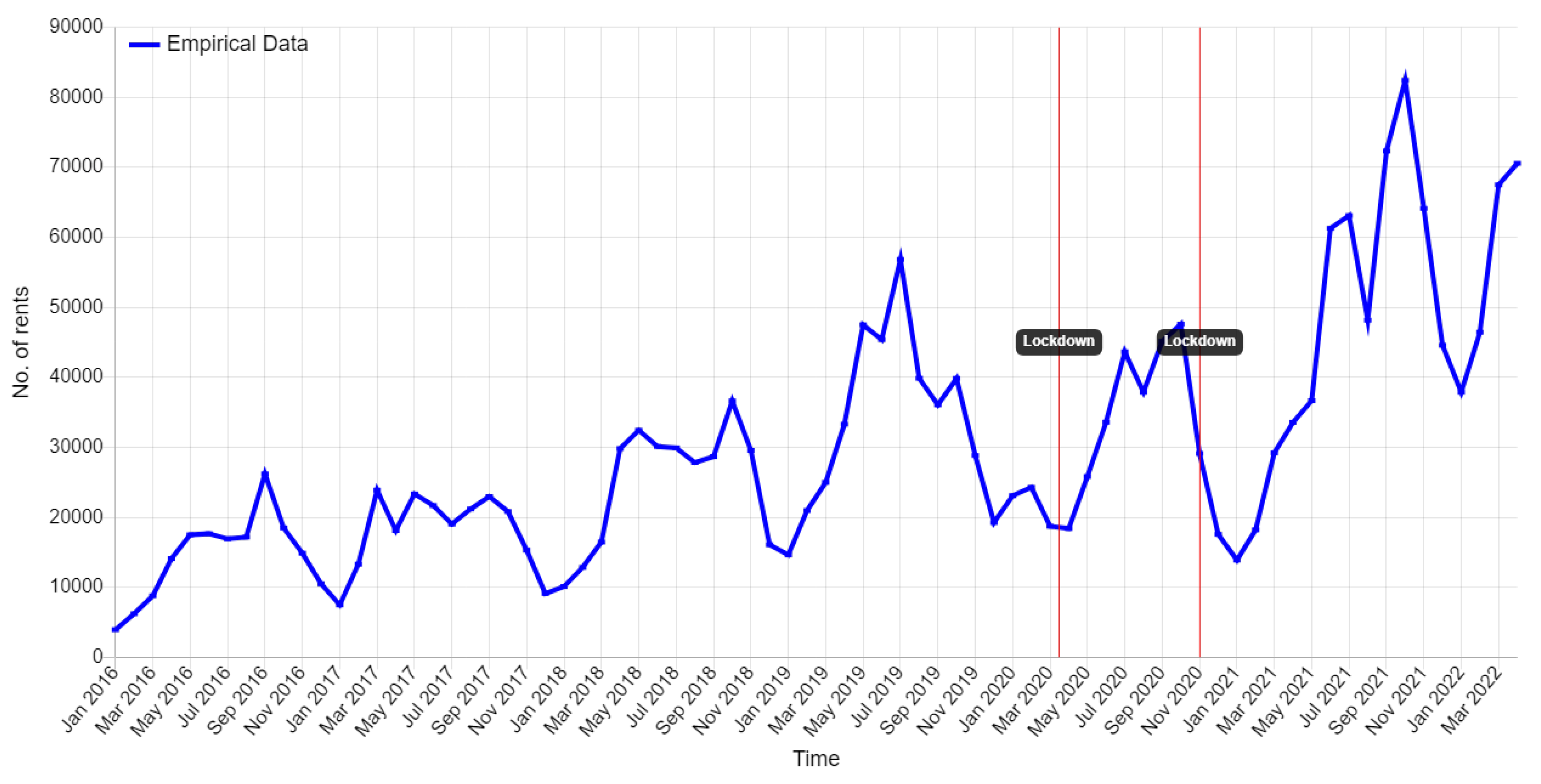
Figure 2 shows the monthly development of the VRNnextbike BSSs. In 2016 and 2017, the absolute number of rentals stagnated between 17,000 and 26,000 in warm months and dropped below 10,000 in cold months. As the system expands, rental numbers increase (2018–2019). The growth is slowed by the COVID-19 pandemic in 2020. With the abolition of COVID-19 restrictions, the number of rentals increases to an all-time high of over 82,000. The data shows typical patterns, thus a positive trend and repeating annual seasonality can be seen over the years. The rental numbers increase in summer time and decrease during the cold months. COVID-19 restrictions in the form of lockdowns, such as the first lockdown (March–June 2020), are also recognizable. This time series of the absolute number of rentals is used as the endogenous dependent variable. This variable is caused by factors within the system and will be predicted by the model.

3.2. Exogenous Factors

Including exogenous factors can improve the model performance. These factors are included as independent effects and are thus not explained by the model. A number of exogenous variables from three categories are available (see

Table 1. Adding exogenous factors can improve model performance. Different exogenous variables from three categories are available: meteorological, system-based and non-system-based data.

Exogenous Variable	Unit	Description
Rain precipitation	mm	Monthly sum of rain precipitation per municipality
Sun hours	Quantity	Monthly sum of sun hours per municipality
Daytime temperature	°Celsius	Monthly arithmetic mean of daytime temperature per municipality
Rental duration (Mean)	Minutes	Monthly arithmetic mean of the rental period per municipality
Rental duration (Sum)	Minutes	Monthly sum of the rental period per municipality
Distance traveled (Mean)	km	Monthly arithmetic mean of distances traveled per municipality
Distance traveled (Sum)	km	Monthly sum of distances traveled per municipality
Corona infections	Quantity	Monthly number of new COVID-19 infections in the supply area
Vacations	Quantity	Monthly number of vacation days and public holidays in the supply area

). The selection of exogenous factors is based both on related work and with discussions with the transport association VRN and the company nextbike.

The first category of effects includes meteorological data such as the daytime temperature, sun hours and rain precipitation. For example, on cloudy days the temperature can be relatively high and, conversely, cold winter days can also have many hours of sunshine. The second category contains system-based data, for example the sum of distances traveled or the arithmetic mean of rental periods. These variables thus reflect user behavior and have a high correlation to the number of bikes in the system. The last category includes non-system-based exogenous factors such as COVID-19 infections or vacations. These variables are needed to account for causal effects such as the COVID-19 pandemic or school vacations, as these change the habitual behavior of users. The individual values were aggregated to monthly numbers and calculated as a sum or arithmetical mean across the VRNnextbike municipalities or specify the respective quantity in the month for the supply area.

The dataset is divided into a training and a validation period. The training period is set from January 2016 to June 2021 and the validation period from July 2021 to April 2022. The initial period from March 2015 to December 2015 is not used. This is due to the small number of stations and number of rentals in the BSS in the aforementioned period. A consistent picture emerges for the exogenous variables from January 2016 on, which also marks the starting point of the training time series. The modeling of the training time series is an in-sample prediction because the data is used to fit the model. This prediction is therefore after referred to as an in-sample prediction. Since the validation period is not known to the model, this is an out-of-sample prediction, after simply called forecast.

4. Models and Model Evaluation

This section introduces the models and their components (Section 4.1, Section 4.2 and Section 4.3). Section 4.4 provides different metrics that are considered in the evaluation of the models.

4.1. Unobserved Component Model

The Unobserved Component Model was introduced by Harvey (1990) [23,24] and is a multiple regression model with time-varying parameters. It is based on the principle that the time series is decomposed into components such as trend, seasonal and irregular component. The generalized model can be defined as follows:

$$UCM:y_t={\mu }_t+{\gamma }_t+c_t+r_t+\sum _{i=1}^k{\beta }_i{x}_{it}+{\epsilon }_{t}t=1,\dots ,n$$

(1)

where $y_t$ is the time series, ${\mu }_t$ the trend component, ${\gamma }_t$ the seasonal component, $c_t$ the cyclical component, $r_t$ the auto-regressive component, ${\epsilon }_t$ the irregular component and the explanatory regression terms ${\sum }_{i=1}^k{\beta }_i{x}_{it}$. The trend component ${\mu }_t$ consist of a stochastic level and a stochastic slope as follows:

$$\begin{array}{c}\hfill {\mu }_t={\mu }_{t-1}+{\beta }_{t-1}+{\eta }_{t-1}{\eta }_t\sim N(0,{\sigma }_{\eta }^2)\end{array}$$

(2)

$$\begin{array}{c}\hfill {\beta }_t={\beta }_{t-1}+{\zeta }_{t-1}{\zeta }_t\sim N(0,{\sigma }_{\zeta }^2)\end{array}$$

(3)

where Equation (2) describes the level ${\mu }_t$, while Equation (3) represents the slope ${\beta }_t$. This allows the level component to change between different points in the time-series, which means that the trend can develop slowly and does not have to be linear [25,26]. The two disturbance terms ${\eta }_t$ and ${\zeta }_t$ are independent of each other with mean zero and variances ${\sigma }_{\eta }^2$ and ${\sigma }_{\zeta }^2$.

Seasonal effects are represented by the seasonal component ${\gamma }_t$. The component depends significantly on the periodicity s, which is set to 12 because of the monthly data. The seasonal pattern can change over time through the independent error term ${\omega }_t$ with variance ${\sigma }_{\omega }^2$ [25]. This results in

$${\gamma }_t=-\sum _{j=1}^{s-1}{\gamma }_{t+1-j}+{\omega }_t{\omega }_t\sim N(0,{\sigma }_{\omega }^2)$$

(4)

for $t=1,\dots ,n$. The season coefficients ${\gamma }_{s-1}$ are initially unknown and are estimated by the model. The cyclical component represents cyclic effects that are not captured by the seasonal component. Typically, the cyclical component is used to model a business cycle [26]. This cycle is defined as follows:

$$\begin{array}{c}\hfill c_{t+1}=p_c({\tilde{c}}_{t}cos{\lambda }_{c}t+{\tilde{c}}_t^{*}sin{\lambda }_c)+{\omega }_t{\omega }_t\sim N(0,{\sigma }_{\tilde{\omega }}^2)\\ \hfill c_{t+1}^{*}=p_c(-{\tilde{c}}_{t}sin{\lambda }_{c}t+{\tilde{c}}_t^{*}cos{\lambda }_c)+{\tilde{\omega }}_t^{*}{\tilde{\omega }}_t^{*}\sim N(0,{\sigma }_{\tilde{\omega }}^2)\end{array}$$

(5)

where $cos{\lambda }_{c}t$ and $sin{\lambda }_c$ are trigonometric functions with frequency ${\lambda }_c$ so that $2\pi ={\lambda }_c$ is the period of the cycle [26]. The independent disturbance terms ${\omega }_t$ and ${\tilde{\omega }}_t^{*}$ have variance ${\sigma }_{\tilde{\omega }}^2$ and zero mean. The cyclic coefficients ${\tilde{c}}_t$ and ${\tilde{c}}_t^{*}$ are determined by the model. The cycle can be additionally damped by the factor $p_c$, but is initially set to $p_c=1$. The auto-regressive component is of form

$$r_t=\varphi \left(L\right)r_{t-1}+{\epsilon }_t^{*}{\epsilon }_t^{*}\sim N(0,{\sigma }_{\epsilon }^2)$$

(6)

where L is the lag operator, $\varphi$ the auto-regressive coefficient and ${\epsilon }_t^{*}$ the disturbance term. The independent terms ${\epsilon }_t$ (see Equation (1)) and ${\epsilon }_t^{*}$ are Gaussian white noise processes and are normally distributed with variance ${\sigma }_{\epsilon }^2$. The lag operator L is the well-known Backshift operator which can be defined as [25]:

$$L^i\left(y_t\right)=y_{t-i}$$

(7)

where i is the order of differencing.

4.2. ARIMAX

In 1976 Box and Jenkins [27] introduced the Auto-Regressive Integrated Moving Average model (ARIMA) for times series prediction. The model consists of an auto-regressive process (AR), a Moving Average process (MA) and an Integrated part. The AR process describes a noisy combination of the previous p-observations of the time series $y_t$, while the MA process defines a noisy combination of previous q-regression errors. The integrated part also enables modeling non-stationary time series by differentiation of order d. The model has three configurable parameters denoted as $(p,d,q)$. The ARIMA model can be extended by exogenous variables, resulting in ARIMAX. The ARIMAX model is defined as follows:

$$ARIMAX(p,d,q):y_t=\sum _{i=1}^{p+d}{\phi }_i{\Delta }^d{y}_{t-i}+\sum _{j=1}^q{\theta }_i{\epsilon }_{t-J}+\sum _{m=1}^M{\beta }_m{x}_{mt}+{\epsilon }_t{\epsilon }_t\sim N(0,{\sigma }_{\epsilon }^2)$$

(8)

for $t=1,\dots ,n$ where ${\sum }_{i=1}^{p+d}{\phi }_i{\Delta }^d{y}_{t-i}$ is the AR process with coefficients $\phi$ and differential operator ${\Delta }^d$ of order d, followed by the MA process ${\sum }_{j=1}^q{\theta }_i{\epsilon }_{t-J}$, consisting of coefficients $\theta$ and disturbance terms ${\epsilon }_q$, and the explanatory regression term ${\sum }_{m=1}^M{\beta }_m{x}_{mt}$ along with disturbance term ${\epsilon }_t$. The differential operator is defined as:

$${\Delta }^d=y_t-y_{t-d}$$

(9)

4.3. SARIMAX

A seasonal component can be added to the ARIMAX model [28]. The seasonality s is modeled by own AR and MA processes and a seasonal integrated part. This results in the seasonal order denoted as $(P,D,Q,s)$. The SARIMAX can be defined as follows:

$$\begin{array}{c}\hfill SARIMAX(p,d,q)x(P,D,Q,s):y_t={\beta }_t{x}_t+u_{t}t=1,\dots ,n\\ \hfill \varphi \left(L\right)\tilde{\varphi }\left(L^S\right){\Delta }^d{\Delta }_s^D{u}_t=\theta \left(L\right)\tilde{\theta }\left(L^s\right){\epsilon }_t{\epsilon }_t\sim N(0,{\sigma }_{\epsilon }^2)\end{array}$$

(10)

where ${\beta }_t{x}_t$ is the explanatory regression term, $\varphi \left(L\right)$ the non-seasonal auto-regressive lag polynomial, $\tilde{\varphi }\left(L^S\right)$ the seasonal auto-regressive lag polynomial, ${\Delta }^d$ the non-seasonal differential operator, ${\Delta }_s^D$ the seasonal differential operator, $\theta \left(L\right)$ the non-seasonal moving average lag polynomial, $\tilde{\theta }\left(L^s\right)$ the seasonal moving average lag polynomial and ${\epsilon }_t$ a Gaussian white noise process and with variance ${\sigma }_{\epsilon }^2$.

4.4. Evaluation and Metrics

The Root Mean Square Error (RMSE) is a frequently used criterion which determines the model accuracy based on the forecast results and the empirical data. RMSE is defined as:

$$RMSE=\sqrt{\frac{{\sum }_{i=1}^n{({\tilde{y}}_i-y_i)}^2}{n}}$$

(11)

where ${\tilde{y}}_i$ is the predicted value, $y_i$ the empirical value and n the number of observations. The RMSE is always non-negative and an RMSE value of 0 would represent a perfect fit to the data. However, RMSE is sensitive to outliers. Hyndman and Koehler [29] introduced the Mean Absolute Scaled Error (MASE) as this is less sensitive to outliers and easier to interpret. Here the model forecast is compared to an in-sample one-step naive forecast. MASE can be defined as follows:

$$MASE=\frac{{\sum }_{t=1}^n\left|\frac{E_t}{\frac{1}{n-m}{\sum }_{t=m}^n|y_t-y_{t-m}|}\right|}{n}$$

(12)

where $E_t$ is the prediction error of the validation data, m the periodicity and n the number of observations. MASE is always non-negative and a value of 0 would represent a perfect fit to the data. MASE $>1$ indicates that the model forecast is poorer than the forecast of the naive method.

When comparing competing models, a fair criterion is required because the models may have a different number of parameters. Therefore, the Akaike information criterion (AIC) and Bayesian information criterion (BIC) are used. These criterions compare the log-likelihood values of the fitted model with the corresponding log-likelihood values of the competing models [25]. Models with more parameters receive a larger penalty, favoring models with smaller parameters and higher log likelihood. AIC and BIC are defined as:

$$\begin{array}{c}\hfill AIC=-2logL\left(Y_n\right|\psi )+2w\end{array}$$

(13)

$$\begin{array}{c}\hfill BIC=-2logL\left(Y_n\right|\psi )+wlogn\end{array}$$

(14)

where $\psi$ is the estimated parameter vector, w the number of estimated parameters and n the number of observations.

5. Model Development

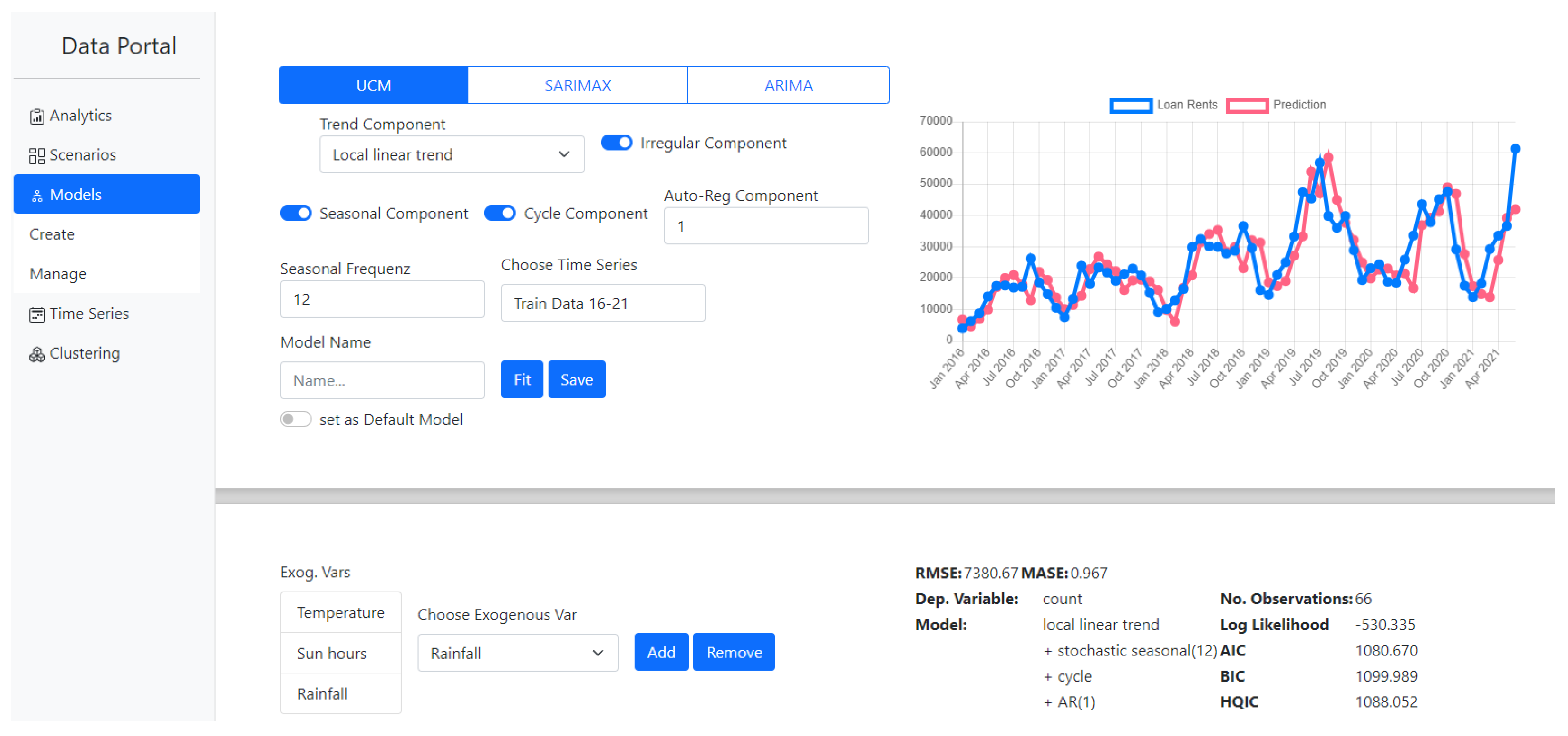
The implementation of the models is realized with the Python package statsmodels [30]. The model implementation is part of the server-backend of the data portal. A web application is available as a graphical user interface (Figure 3).

The UCM model is implemented as a traditional state space model, thus the model parameters are obtained by maximum likelihood estimation via Kalman filtering. The well known Kalman filter [25,26,31] allows one-step ahead forecasts. The filter is a recursive technique that improves the estimated parameters with each new observation. The forecast $y_{n+1}$ can be estimated from given $y_1,\dots ,y_n$ by applying the Kalman filter for $t=1,\dots ,n,n+1$.

Initially, a set of different univariate UCMs were explored to find the best possible combination of components. The first model set (Set 1) contains an UCM with all components as described in Section 4.1 and serves as the baseline. The baseline UCM has a trend (level + slope), seasonal ($s=12$), cyclical ($p_c=1$), auto-regressive (AR(1)) and an irregular component. The second set corresponds to the baseline UCM but without the seasonal component (Set 2). The third set replicates the baseline model, but does not have a cyclic component (Set 3). Experiments were also carried out with different modeling of the trend component. A fixed intercept (Equation (15)) and a fixed slope (Equation (16)) were considered for trend modeling. Such models are defined as:

$$\begin{array}{c}\hfill {\mu }_t=\mu t=1,\dots ,n\end{array}$$

(15)

$$\begin{array}{c}\hfill {\mu }_t={\mu }_{t-1}+\beta t=1,\dots ,n\end{array}$$

(16)

where $\beta$ is the fixed slope and ${\mu }_n$ the trend coefficients. Compared to the baseline, Set 4 has no cyclic component and a fixed intercept as trend component. On contrast, Set 5 has a fixed slope as trend component and a cyclic component. Additionally, higher AR orders were evaluated. Thus, it was found that low AR orders (such as AR(1)) are often sufficient and higher AR orders rarely increase the performance of the models. As a consequence, all sets have an AR(1)-process, except for Set 5 which has an AR order of 4.

Table 2. Evaluation of different component sets for univariate UCMs. Removing the cyclic component significantly increases forecast performance (Set 3). Best results were achieved with Set 5 (fixed slope + AR(4)-process).

Criterion	Set 1	Set 2 ${}^{†}$	Set 3 ${}^{‡}$	Set 4 ${}^{‡,}$*	Set 5 ${}^{\mp ,}$**
AIC	1082	1346	1116	1133	1065
BIC	1095	1357	1128	1143	1079
RMSE
In-Sample	8067	8177	7576	7461	7071
Forecast	77,740	87,733	13,197	11,586	12,293
MASE
In-Sample	1.084	1.12	0.984	0.949	0.995
Forecast	11.71	13.2	1.89	1.80	1.71

^† without seasonal component ^‡ without cyclic component * fixed intercept ** fixed slope ^∓, AR(4).

summarizes various model sets and their performance.

The UCM without a seasonal component (Set 2) performed worse in all metrics. Better results were obtained without the use of a cyclic component (Set 3). The forecast performance in particular was significantly improved. The RMSE was reduced by a factor of 6.6 and the MASE by a factor of 6.9. Experiments to estimate the damped factor of the cyclic component as an additional parameter did not yield a significant improvement. Set 4 with fixed intercept trend and no cyclical component achieved slightly better in-sample and forecast performance, but at the expense of model quality. The lowest AIC and BIC values and the best forecast MASE score could be achieved for an univariate UCM with Set 5.

For the development of the multivariate model different feature sets (FS) were formed from the available exogenous variables. The first feature set (FS1) contains all exogenous factors and serves as the baseline. The second FS includes only meteorological variables (FS2) and the third contains only system-based factors (FS3). A grid search [32] was performed to identify additional sets. For this purpose, a search space was defined, which consists of all different possible combinations of the exogenous variables. The grid search then tries out all combinations from the search space and filters the results according to the forecast quality. As a result, two more promising sets were found (SF4 & SF5). Thus, the experiments found that exogenous factors such as the number of vacations or COVID-19 counts did not significantly affect the model’s forecasting quality. The influence of COVID-19 and its use as an exogenous factor is further discussed in Section 6. SF4 contains only one variable (summed rental duration), while SF5 is a mixed set consisting of the mean traveled distance, rain precipitation, sun hours and daytime temperature. The different feature sets were evaluated using the baseline UCM model with all components and an AR(1)-process (see

Table 3. Evaluation of exogenous feature sets using the baseline UCM. The addition of exogenous variables increases the performance of both the in-sample prediction and the forecast. The best forecast was obtained with the mixed Feature Set 5.

Criterion	FS 1 ${}^{†}$	FS 2 ${}^{‡}$	FS 3 ${}^{\mp ,}$	FS 4 *	FS 5 **
AIC	1093	1080	1032	911	1077
BIC	1124	1099	1054	926	1098
RMSE
In-Sample	2609	7380	2675	1073	7242
Forecast	51,053	31,167	50,592	34,149	9460
MASE
In-Sample	0.296	0.967	0.315	0.141	1.013
Forecast	8.37	4.24	8.31	5.54	1.38

^† all exogenous factors ^‡ only meteorological ^∓, only system-based * summed rental duration ** mean traveled distance, rain precipitation, sun hours, daytime temperature.

). For the forecast, exogenous variables were estimated from the mean of the last two years.

The multivariate baseline (FS 1) has significantly low values for the error metrics compared to the univariate baseline (Set 1). The RMSE decreases from 8067 to 2609 for the in-sample prediction, as well the MASE score from 1.084 to 0.296. However, the forecast performance increases only slightly and the AIC/BIC values increase slightly due to the additional exogenous model parameters. By considering only meteorological variables (FS 2), the forecast errors decrease and the model quality increases slightly, but at the expense of the in-sample performance. Including only system-based variables (FS 3) did not improve performance over baseline. Feature Set 4 achieved the best in-sample results together with the lowest AIC/BIC values. However, the forecast performance is slightly weaker than FS2. The mixed Feature Set 5 achieved a moderate in-sample performance, but convinced due to the lowest error values in the forecast. Based on the feature sets, experiments were carried out with different component combinations to further improve the model quality, but no performance improvement could be found. Results of statistical tests for uni- and multivariate UCMs can be found in the Appendix A (

Table A1. Statistical test of UCM-components (univariate baseline model as described in Section 5).

Component	z-Value	p > |z|
Irregular	0.122	0.903
Level	1.529	0.126
Trend	1.376	0.169
Seasonal	1.009	0.313
AR	287.169	0.000
Cycle	1.278	0.201

and

Table A2. Statistical test of UCM-components (multivariate model with FS 5 as described in Section 5).

Component	z-Value	p > |z|
Irregular	0.147	0.883
Level	0.312	0.755
Trend	0.725	0.468
Seasonal	2.196	0.028
AR	31.346	0.000
Cycle	0.001	0.999
Mean traveled distance	−0.768	0.443
Rrain precipitation	−0.246	0.806
Sun hours	−0.613	0.540
Daytime temperature	3.887	0.000

).

6. Results

To evaluate the different models, the performance of the in-sample and the forecast (out-of-sample) are compared. The orders of the ARIMA and SARIMA models were determined using grid search. For each parameter of the order a search space was defined (e.g., interval 0-12). Then all possible order combinations were evaluated to find the best possible order for each model. For the multivariate models, the search space was extended by the exogenous feature sets defined in Section 5. The models were selected based on their forecast performance. An overview of the results is provided in

Table 4. Overview of in-sample predictions and forecasted results of ARIMA(X), SARIMA(X) and UCM(X) models. The baseline UCM with Feature Set 5 achieves the best forecast performance.

Criterion	ARIMA 1	ARIMAX 2	SARIMA 3	SARIMAX 4	UCM 5	UCM(X) 6
AIC	1353	1362	1121	1105	1065	1077
BIC	1390	1414	1184	1127	1079	1098
RMSE
In-Sample	5632	5094	6206	6308	7071	7242
Forecast	14,596	13,054	21,774	11,938	12,293	9460
MASE
In-Sample	0.781	0.824	0.714	0.790	0.821	1.013
Forecast	2.30	1.90	3.15	1.72	1.71	1.38

¹ Order (4, 1, 12) ² Order (7, 1, 12) + FS 5 ³ Order (8, 1, 8)x(6, 1, 9, 12) ⁴ Order (2, 1, 1)x(2, 1, 2, 12) + FS 2 ⁵ Fixed slope, seasonal and cyclic component, AR(4) ⁶ Baseline + FS 5.

.

The evaluation shows that the forecast performance of multivariate models is better than with univariate models. In detail, the ARIMAX model improves his forecast performance by 10.56% (RMSE) and 17.39% (MASE) compared to its univariate variant, but shows a deterioration in the AIC/BIC criterion. The SARIMAX model in particular benefits from exogenous factors. Here, the error metrics show a reduction of 45.17% (RMSE) and 45.39% (MASE) compared to SARIMA model. However, the best forecast is provided by the UCM which also has the best model goodness of fit in terms of AIC/BIC values. In detail, the UCMX provides the best forecast RMSE value of 9460 and a MASE value of 1.38, which is an improvement of 20.76% (RMSE) and 19.76% (MASE) over SARIMAX. Compared to ARIMAX, the reduction in error metrics is about 27%.

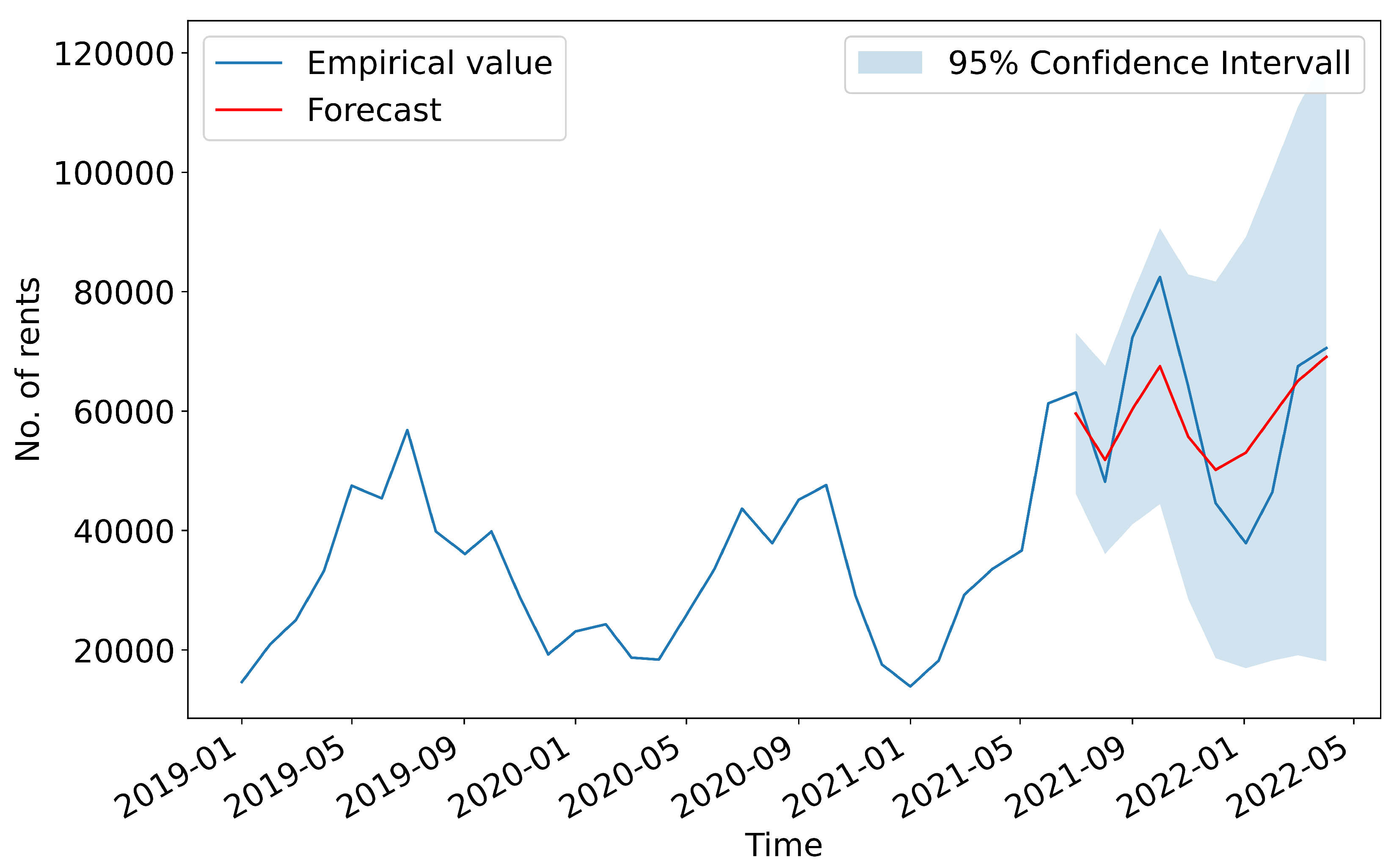
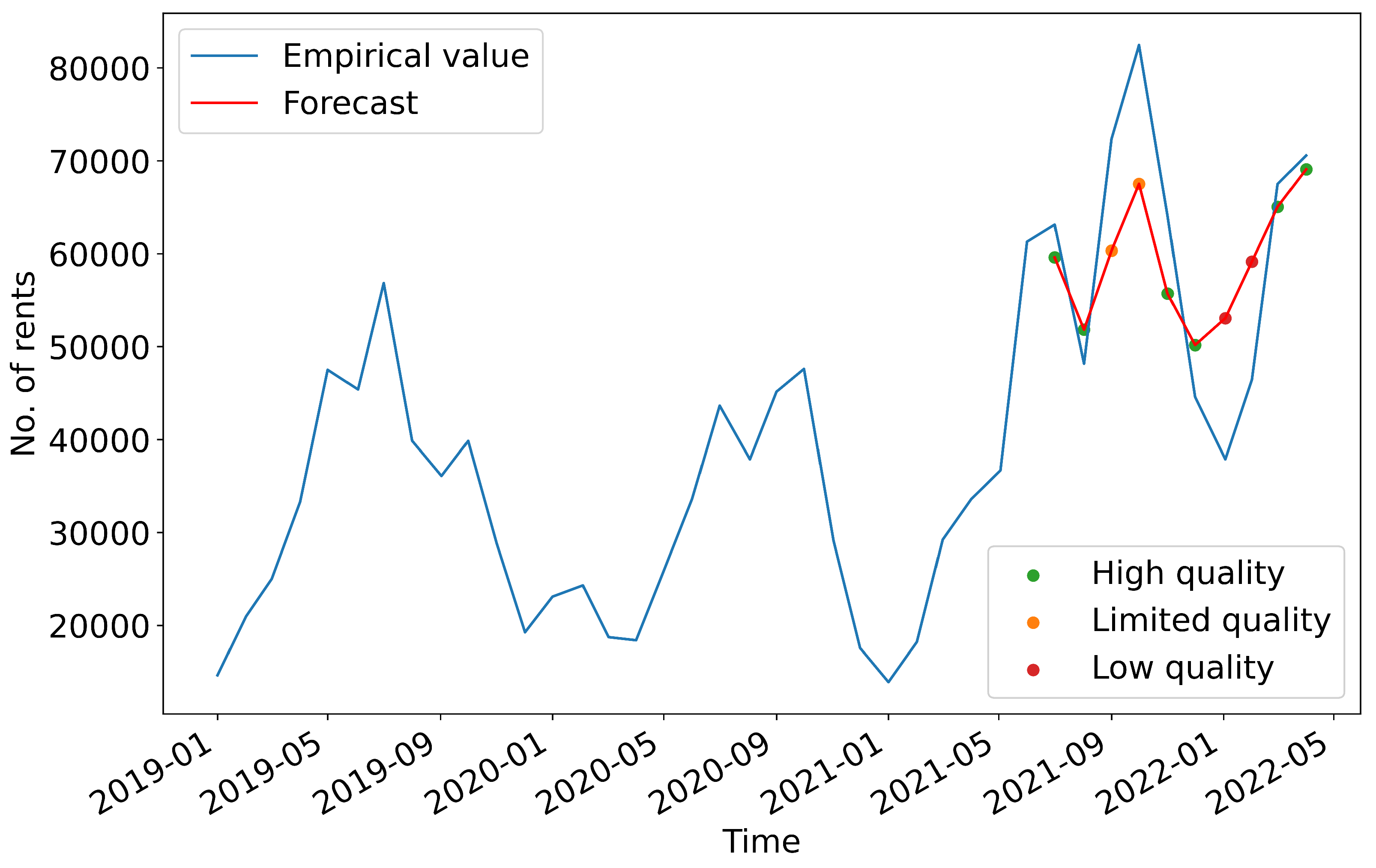
Figure 4 shows the results of the UCM(X) forecast and the associated 95%-confidence interval. As described in Section 3.2 the training period is set from January 2016 to June 2021 and the forecast period from July 2021 to April 2022. The forecasts are within the confidence interval and approach the empirical values.

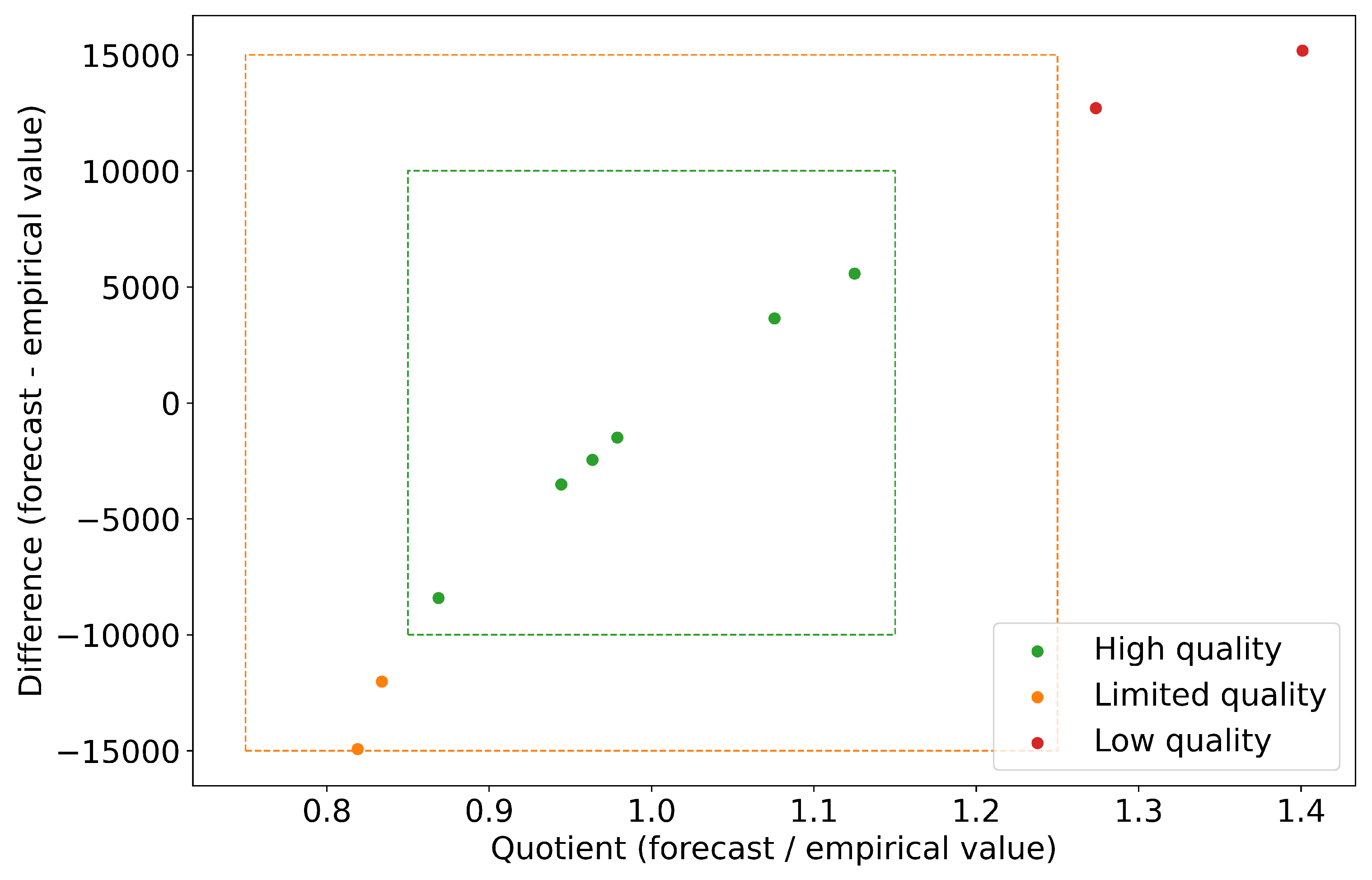
In order to be able to evaluate the forecast quality on a monthly basis more precisely, a consideration of the absolute and relative differences between the empirical and predicted values is used. Three quality levels for residuals were defined and mapped to the forecast. The levels are defined as high, limited and low quality. The quality is determined on the basis of two key indicators. The first indicator is the difference between predicted and empirical value, while the second indicator is the quotient of predicted and empirical value. High quality is achieved if the forecast value does not fall below or exceed the threshold value of 10,000 rentals. A 30% interval is specified for the quotient, which means that the forecast value may deviate by a maximum of 15% upwards or downwards from the empirical value. The forecast quality is limited if the difference is between 10,000 and 15,000. For the quotient, the interval is extended to 50%. This means that the forecast values may deviate upwards or downwards by more than 15%, but not more than 25%. The forecast is of low quality if the threshold of 15,000 for the difference and the 50% interval are exceeded. The threshold values for the evaluation of the residuals were chosen arbitrarily. The evaluation of forecast quality in other scientific fields or applications might demand other thresholds or more elaborate statistical methods.

Figure 5 shows the quality levels of the forecasts based on the previously defined indicators by mapping the calculated quality to each forecast data point. The residuals are calculated based on the deviation in the difference between the forecast and empirical value. Figure 6 indicates the forecast quality of the UCMX model based on the residuals and the quotient, as well as the set bounds.

The evaluation shows that the forecast quality of the model is mostly high. The forecast for the first two months July and August deviates by only about 3000 rentals. The months of transition from summer to autumn (September/October), however, have limited quality. Here, the deviation of the forecast from the empirical values is 12,000 and 14,000. For these months, the empirical values are underestimated. A low forecast quality can been observed in the winter months (January and February), as the deviation with values of over 16.000 exceeds the threshold for moderate forecast quality. The empirical values are significantly overestimated.

As noted in Section 3.1, the COVID-19 pandemic had an impact on BSS and its rental activities. In a previous study, it was found that the effects of COVID-19 restrictions varied for BSS [33]. Thus, more rental bikes were used in the second lockdown (November 2020–June 2021) than in the first lockdown (March–June 2020), although the restrictions on the population were significantly increased in the second lockdown. This fact could explain why the COVID-19 numbers as an exogenous factor had no significant influence on the model. After the restrictions were gradually lifted from June 2021, the number of rentals grew considerably, so the empirical values are underestimated.

7. Discussion & Conclusions

The main objective of this paper was to evaluate the feasibility of UCMs for long term forecasting using a dataset of a bike sharing service. The proposed UCM model outperforms ARIMA, ARIMAX, SARIMA and SARIMAX in terms of out-of-sampling forecasting in all metrics. The results show that UCM is a promising statistical approach for the prediction of BSS rentals. Our experiments also show that multivariate models that include exogenous factors as independent effects have better predictive performance than their univariate counterparts. The experiments reveal that a mixed set of exogenous factors, consisting of meteorological (temperature, sun hours, rain precipitation) and system based variables (mean traveled distance), has a significant impact on forecast quality. No significant influence was found for COVID-19 numbers or the number of vacation days as an exogenous factor.

The results of the models could be further improved by enhancing the estimation of the exogenous variables for the validation/out-of-sample period. Linear regression models or custom UCMs could be used for estimation and more adequate forecast scenarios. Another possibility could also be that the required forecasts come from external sources. Thus, a cooperation with meteorological institutes, that have more specialized models to predict weather data for a future period, would be conceivable.

Another approach to improving performance would be to add new and different exogenous factors. For example, an indicator for university semester breaks would be an option, since BSSs are often used by students who represent a large user group. Indicators of local road traffic congestion or promotional activity for the BSS could also be helpful.

The scope for improvement in univariate ARIMA and SARIMA models is limited. Here, statistically irrelevant lag-variables could be removed for high order AR or MA processes.

Future work may address the above mentioned suggestions and also explore different directions as well. A next step would be to compare the UCM with other models, especially machine learning models such as LSTMs, TCNs or Gradient Tree Boosting Systems. The LTSF-Linear Model [34] should also be mentioned, which outperforms existing Transformer-based LTSF solutions and thus represents the state of the art in the field of ML-forecast-models. Other work could investigate the performance of the UCM for short term or station-based predictions.