PG-Based Vehicle-In-the-Loop Simulation for System Development and Consistency Validation

Abstract

The concern over safety features in autonomous vehicles is increasing due to the rapid development and increasing use of autonomous driving technology. The safety evaluations performed for an autonomous driving system cannot depend only on existing safety verification methods, due to the lack of scenario reproducibility and the dynamic characteristics of the vehicle. Vehicle-In-the-Loop Simulation (VILS) utilizes both real vehicles and virtual simulations for the driving environment to overcome these drawbacks and is a suitable candidate for ensuring reproducibility. However, there may be differences between the behavior of the vehicle in the VILS and vehicle tests due to the implementation level of the virtual environment. This study proposes a novel VILS system that displays consistency with the vehicle tests. The proposed VILS system comprises virtual road generation, synchronization, virtual traffic manager generation, and perception sensor modeling, and implements a virtual driving environment similar to the vehicle test environment. Additionally, the effectiveness of the proposed VILS system and its consistency with the vehicle test is demonstrated using various verification methods. The proposed VILS system can be applied to various speeds, road types, and surrounding environments.

1. Introduction

Autonomous driving systems have been developed rapidly in recent years to achieve the goal of full autonomy. As technology advances, various systems are complexly linked to each other, and verifying the safety of autonomous driving systems will become increasingly important [1]. Consequently, various research institutes and governments are conducting extensive research on the development of related technologies and the verification of the safety of autonomous driving systems. Unlike the existing SAE Lv.2 level Advanced Driver Assistance System (ADAS), an autonomous driving system must respond to various situations on the road independently, and any accidents that occur are attributed to the vehicle instead of the driver [2]. To ensure the safety of the drivers in such systems, an effective safety verification method must be developed by testing the systems over millions or even billions of kilometers [3,4,5]. The safety verification testing methods are largely divided into simulation-based testing and vehicle testing. Currently, various simulation-based testing methods are being used, which include Model-In-the-Loop (MIL), Software-In-the-Loop (SIL), and Hardware-In-the-Loop (HIL) [6]. MIL and SIL are useful for testing algorithms quickly because the vehicle, sensor, actuator, and controller all consist of virtual models. Additionally, SIL can be implemented to test the software of an algorithm mounted on a vehicle, and verification can be performed at the ECU level without using an actual ECU. HIL can be implemented at the level of actual ECUs and hardware, and real-time verification, including verification of the characteristics of actual hardware, can be performed by including actual hardware such as sensors and actuators in the simulation. However, in the simulation-based testing method, there may be errors between the behavior of the actual vehicle and its dynamic characteristics due to the application of the virtual vehicle dynamics model and to the occupants being unable to feel the vehicle’s behavior. Vehicle testing is the final step in verifying the effectiveness of the autonomous driving algorithm because it uses a real vehicle, along with real sensors and a real surrounding environment [7]. The effectiveness of the existing body control system and chassis control system can be verified through vehicle testing in the stage just before commercialization after the development process. However, verifying the effectiveness of the autonomous driving system, which responds to various dangerous traffic situations during the vehicle test, is difficult due to the expansion of Operational Design Domain (ODD). Vehicle testing requires various external factors such as the surrounding environment and objects, due to which it cannot be performed by the vehicle alone. Even if a test bed and several dummy obstacles such as vehicles and pedestrians are prepared at a high cost, it is not possible to replicate a specific scenario during the vehicle test; there is also a risk of collision with the surrounding objects [8].

Therefore, Vehicle-In-the-Loop Simulation (VILS), which is a verification method based on virtual environments and real vehicles, has gained considerable interest as a means to overcome the limitations of the simulation and vehicle testing methods. VILS can ensure repeatability and reproducibility and can considerably reduce the risk of collisions when compared to vehicle tests because the surrounding objects and environments are represented as virtual objects, as shown in

Table 1. Comparison of various testing methods for a vehicle.

Testing Method	Vehicle Dynamics	Cost	Reproducibility	Danger
MIL	Model	Low	High	Low
SIL	Model	Low	High	Low
HIL	Partial Model	Mid	High	Low
Vehicle Test	Real	High	Low	High
VIL	Real	Mid	High	Low

. This method enables the verification of the effectiveness of an autonomous driving system and reflects the dynamic characteristics of the actual vehicle, unlike the existing simulation test methods, such as MIL, SIL, and HIL. Furthermore, the cost required to prepare the test environment is also reduced, thereby improving the economic efficiency.

VILS is divided into dynamo-VILS, which test vehicles on a fixed chassis dynamo, and PG-VILS, which are based on vehicles driving on a Proving Ground (PG) [9]. Related studies can be categorized according to the two different types of VILS. First, the related studies for dynamo-VILS are as follows.

Gletelink [10] proposed a method to verify the effectiveness of the Adaptive Cruise Control (ACC) function by attaching a vehicle to a dynamo and integrating a real robot target vehicle with a virtual surrounding vehicle within a limited indoor space (200 m × 40 m). Rossi [11] analyzed the energy efficiency of a verification vehicle using a dynamo-based ADAS test system called SERBER. Additionally, an Over-The-Air (OTA) sensor emulation method that uses a screen to project an image was employed to ensure that the camera sensor can directly capture an image of the virtual environment. Sieg [12] and Diewald [13] also tested the ADAS and autonomous driving functions using the dynamo and OTA-based radar emulation. Diewald developed a radar OTA emulation method for multiple objects and conducted a VILS test using a radar virtual model capable of replicating real conditions. Gao [14] developed an indoor dynamo-VILS environment and evaluated the performance of autonomous vehicle via Autonomous Emergency Braking (AEB) functions through the developed VILS environment. Zhang [15] also evaluated and analyzed the Energy Management Strategy (EMS) of Hybrid Electric Vehicles (HEV) through dynamo-VILS.

Unlike in the vehicle test, the dynamo-VILS used in the above study was tested in an indoor space, which enables flexible and repeatable testing based on a virtual environment. However, building the dynamo and emulator equipment for each sensor is extremely expensive and requires a large amount of space. Furthermore, the steering angle is limited due to the mechanical link of the dynamo, which requires additional equipment for testing [9].

In the case of the PG-VILS, the vehicle runs on the actual PG, and the vehicle dynamic characteristics are identical to those in the vehicle test, as shown in Figure 1. The acceptance of an autonomous driving system can be evaluated by the passengers in the vehicle. Additionally, the cost of building an environment is significantly lower when compared to dynamo-VILS. Therefore, an efficient verification environment can be configured and unexpected situations on the road, such as traffic congestion, can be virtually realized to verify the effectiveness of the autonomous driving function. The studies related to PG-VILS are as follows.

Park [16] confirmed the validity and safety of the VILS method by establishing a VILS verification environment and performing an ADAS evaluation based on the EuroNCAP test scenarios. Kim [17] conducted tests using VILS in situations that were difficult to verify due to the high risk of collision, such as crossing vehicles and pedestrians on the road. He employed a PG with sufficient width to eliminate the risk of an accident during the test. Tettamanti [18] implemented various traffic scenarios by integrating the VILS environment, which is a virtual realization of an actual test bed, with SUMO, a traffic simulator. Lee [19] verified the effectiveness of Cooperative Adaptive Cruise Control (CACC) using a real vehicle and a virtual vehicle implemented using VILS. Kim [20] and Solmaz [21] constructed a virtual road environment and verified the effectiveness of the lane change algorithm through PG-VILS.

As above, various studies related to dynamo-VILS and PG-VILS have been conducted. The previous studies were primarily focused on the methodology related to VILS implementation or the verification of the target system results using VILS. As a result, there is insufficient research on securing the driving environment at the time of vehicle test and analyzing the consistency of VILS. Therefore, this study aims to verify the effectiveness of an autonomous driving system by establishing a test system using a PG-VILS. A VILS system that can reproduce the driving conditions during the vehicle test was developed, and the validity of the proposed VILS system is analyzed based on the consistency between the vehicle tests and VILS tests. The remainder of this paper is organized as follows. Section 2 describes the overall configuration of the proposed VILS system and presents the details of the system components used to improve the consistency of the vehicle and VILS tests. Section 3 describes the test vehicle used for the VILS applications, and Section 4 describes the procedure and verification method used to verify the consistency of the test results. In Section 5, the performance of the proposed VILS system is verified by comparing the consistency of the VILS test and vehicle test results. Section 6 presents the conclusion of the article along with future research implications.

2. Proposed PG-Based Vehicle-In-the-Loop Simulation System Structure

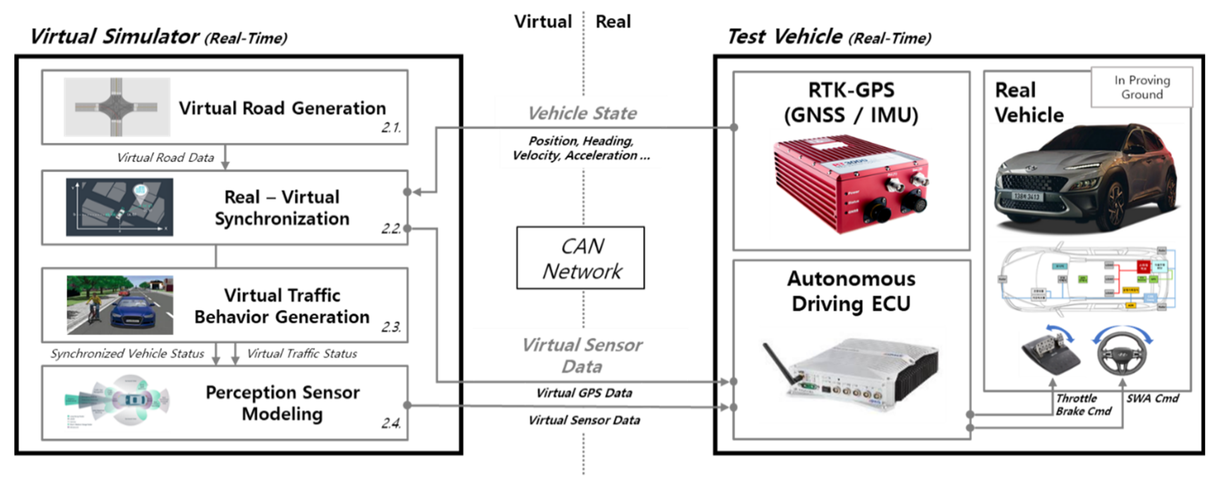
The composition of the proposed VILS system is divided into a virtual simulator and test vehicle, as shown in Figure 2. The virtual simulator comprises four components: virtual road generation, real–virtual synchronization, virtual traffic behavior generation, and perception sensor modeling. The test vehicle is a real vehicle equipped with an autonomous driving ECU which performs autonomous driving using the data generated in a virtual simulator.

Data transmission/reception between the virtual simulator, which generates the virtual environment, and the test vehicle, which operates in the actual proving ground environment, is performed using the CAN communication interface. The state information (position, heading, speed, etc.) which is measured by the RTK-GPS of the test vehicle is transmitted to the virtual simulator to enable interworking between the two environments. Subsequently, the virtual GPS and sensor data of the virtual simulator which are required for autonomous driving control are transmitted to the ECU of the test vehicle. The virtual simulator consists of four elements: Virtual Road Generation, Synchronization, Virtual Traffic Behavior generation, and perception sensor modeling. Virtual Road Data is used for synchronization between real and virtual. Perception sensor modeling is performed by utilizing the state information of the synchronized test vehicle and the behavior of virtual traffic. This study aims to perform a simulation similar to the vehicle test conditions through the proposed processes. This section explains the four elements that constitute the virtual simulator. The next, Section 3, explains the configuration of the test vehicle and presents a detailed explanation of the autonomous driving algorithm applied in this study.

2.1. Virtual Road Generation

To conduct a driving test in a virtual environment, a virtual road environment is required in which to drive the vehicle [22]. In this study, a virtual road was created using HD-MAP, which was provided by the National Geographic Information Institute (NGII) of South Korea. HD-MAP is an electronic map which was developed using the recognition and positioning sensor data installed in a Mobile Mapping System (MMS) vehicle; it provides precise locations and road object property information in centimeters. HD-MAP is essential for autonomous driving systems, which require precise control of the vehicle to perform operations such as lane changes and obstacle avoidance. It differs from navigation and ADAS maps, which can only distinguish the road units [23]. The virtual road environment was developed using the HD-MAP of K-City, an autonomous driving testbed at the Korea Automobile Testing and Research Institute (KATRI).

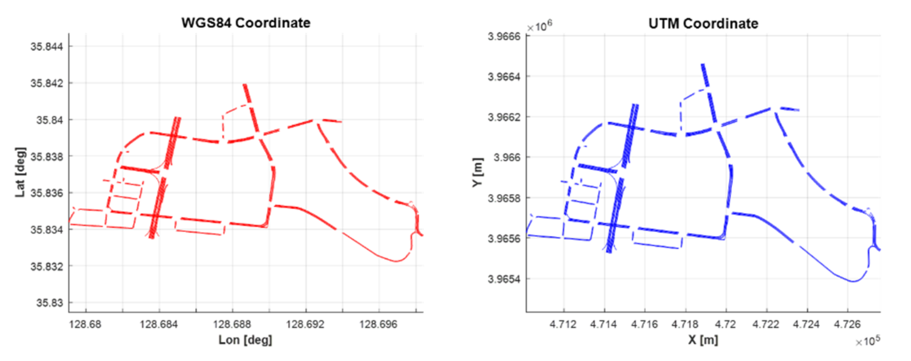
The road shape information provided by the HD-MAP is supported by the World Geodetic System 1984 (WGS84) coordinate system format. Here, the location on the surface of the earth is expressed in terms of latitude and longitude using units of [°], which makes it less useful and intuitive when implementing an autonomous driving system [24]. Therefore, the map must be converted to the Universal Transverse Mercator (UTM) coordinate system in meters, with precision expressed in terms of latitude and longitude. It is easy to express the distance and direction in the case of UTM because all the coordinates on the surface are expressed as X[m] and Y[m] coordinates based on a specific origin. The process of converting the WGS84 coordinate system into UTM coordinates is given as follows [25]:

$$X=k_{0}N[A+(1-T+C)\ast A^3/6+(5-18T+T^2+72C-58e{\prime }^2)A^5/120]$$

(1a)

$$\begin{array}{l}Y=k_0[M-M_0+N\tan \varphi [A^2/2+(5-T+9C+4C^2)A^4/24+\\ (61-58T+T^2+600C-330e{\prime }^2)A^6/720]]\end{array}$$

(1b)

$$\begin{array}{l}M=a[(1-e^2/4-3e^4/256-\dots )\varphi -(3e^2/8+3e^4/32+45e^6/1024+\dots )\sin 2\varphi \\ +(15e^4/\dots +45e^6/1024+\dots )\sin 4\varphi -(35e^6/3072+\dots )\sin 6\varphi +\dots ]\end{array}$$

(1c)

$$\begin{array}{l}{k}_0=0.9996,e^2=(a^2-b^2)/a^2,e{\prime }^2=e^2/1-e^2,N=a/\sqrt{1-e^2{\sin }^2\varphi },\\ T={\tan }^2\varphi ,C=e{\prime }^2{\cos }^2\varphi ,A=(\lambda -{\lambda }_0)\cos \varphi \end{array}$$

(1d)

Here, $k_0$ represents the UTM Central meridian scale factor, and $a$ and $b$ represent the semi-major and semi-minor axes of Earth’s ellipsoid, respectively. $e$ denotes the first eccentricity and $e\prime$ denotes the second eccentricity. $\varphi$ and $\lambda$ represent the latitude and longitude, respectively, and ${\varphi }_0$ and ${\lambda }_0$ represent the origin constants of latitude and longitude.$M$ denotes the actual distance from the equator to latitude based on the central meridian, and $M_0$ denotes the value obtained by applying ${\varphi }_0$ to Equation (1c).

Figure 3 presents an example result obtained when the road shape information of the HD-MAP, which is provided as latitude and longitude in degrees units, is converted into the UTM coordinate system in meter units. The converted road shape information was applied to the IPG Carmaker Scenario Editor to build a virtual road environment.

2.2. Real–Virtual Synchronization

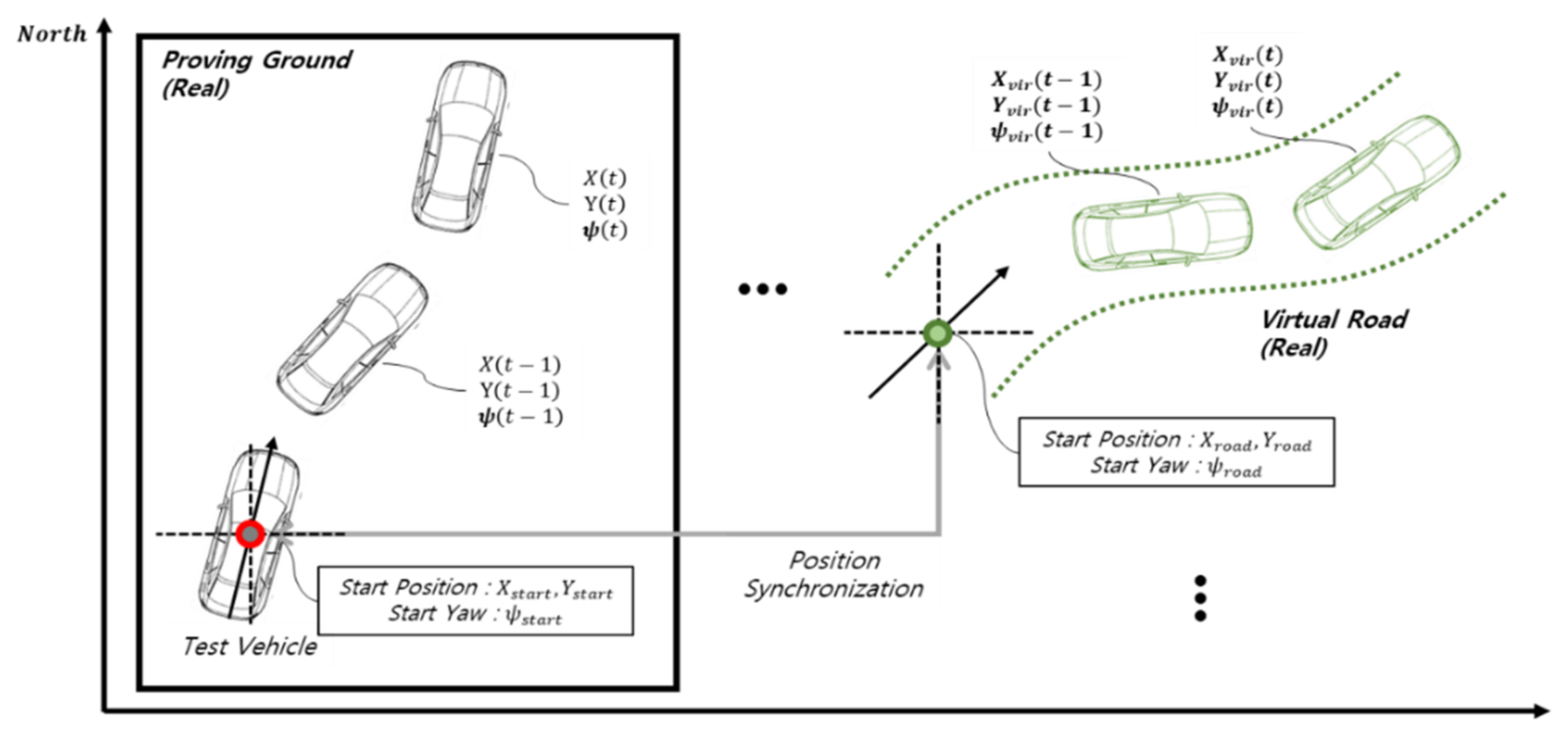
In the case of PG-based VILS, the actual location of the test vehicle and the location of the virtual road do not match. Therefore, the test vehicle must be positioned on the virtual road for the driving test, as shown in Figure 4.

The location information for the test vehicle at the start of the simulation and the location information (position, heading) errors for the starting point of the virtual road were applied to the location information for the test vehicle for each sample using the same process as in Equation (2).

$$X_{vir}(t)=X(t)-(X_{start}-X_{road})$$

(2a)

$$Y_{vir}(t)=Y(t)-(Y_{start}-Y_{road})$$

(2b)

$${\psi }_{vir}(t)=\psi (t)-({\psi }_{start}-{\psi }_{road})$$

(2c)

In this equation, ${()}_{road}$ represents the starting point of the virtual road and ${()}_{start}$ represents the point where the test vehicle is located at the start of the simulation. ${()}_{vir}$ represents the virtual location information, where $X$, $Y$, and $\psi$ represent the X/Y global position and heading value of the vehicle, respectively.

Thus, the location information of the test vehicle is converted into virtual location information to ensure that the vehicle can be driven on a virtual road regardless of the actual location. Since the location information measured by the RTK-GPS of the test vehicle is provided in terms of latitude and longitude, the coordinate system transformation described in Section 2.1 is performed.

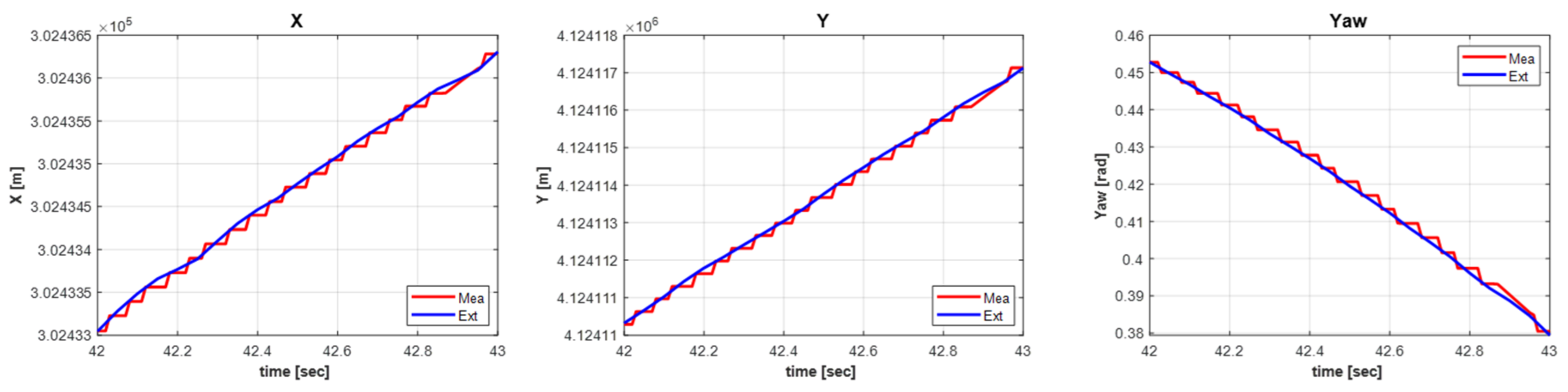
The measurement period (10 Hz–50 Hz) [26,27,28] of the RTK-GPS sensor differs from the period in which the virtual simulator operates (>100 Hz) [29,30,31]. This causes the test vehicle behavior to be updated continuously in the virtual simulator. To achieve an accurate simulation, location information for the test vehicle which matches the cycle of the virtual simulator must be updated continuously. In this study, location information was generated using the extrapolation method based on the operation period of the virtual simulator, as shown below [32]:

$$\begin{array}{l}{v}_{x\_ext}(t)=v_{x\_ext}(t-1)+\{a_{x\_mea}+\frac{(x_{mea}-x_{ext}(t-1))\ast \kappa }{\Delta t_{sim}{}^2}\}\ast \Delta t_{sim},\\ x_{ext}(t)=x_{ext}(t-1)+\{v_{x\_ext}(t)+\frac{(x_{mea}-x_{ext}(t-1))\ast \kappa }{\Delta t_{sim}}\}\ast \Delta t_{sim}\end{array}$$

(3a)

$$\begin{array}{l}{v}_{y\_ext}(t)=v_{y\_ext}(t-1)+\{a_{y\_mea}+\frac{(y_{mea}-y_{ext}(t-1))\ast \kappa }{\Delta t_{sim}{}^2}\}\ast \Delta t_{sim},\\ y_{ext}(t)=y_{ext}(t-1)+\{v_{y\_ext}(t)+\frac{(y_{mea}-y_{ext}(t-1))\ast \kappa }{\Delta t_{sim}}\}\ast \Delta t_{sim}\end{array}$$

(3b)

$${\psi }_{ext}(t)={\psi }_{ext}(t-1)+\{{\gamma }_{mea}+\frac{({\psi }_{mea}-{\psi }_{ext}(t-1))\ast \kappa }{\Delta t_{sim}}\}\ast \Delta t_{sim}$$

(3c)

Here, ${()}_{ext}$ and ${()}_{mea}$ represent the extrapolation value and the measured value, respectively, $\kappa$ represents the filtering constant, and $\Delta t_{sim}$ represents the operation cycle of the simulation. The parameters $x,y,v_x,v_y,a_x,a_y, \psi , \gamma$ represent the global position, longitudinal/lateral speed, acceleration, heading, and heading change rate of the test vehicle, respectively.

The period of the RTK-GPS data measurement value is lower than the period of the simulation, due to which the data are represented in a step shape, as shown in Figure 5. However, continuous position information for the test vehicle which is suitable for the simulation period is generated using the extrapolation method.

2.3. Virtual Traffic Behavior Generation

Ensuring the accuracy of the behavior of the test vehicle used in the simulation test is important. However, in the case of an autonomous driving system simulation, it is also important to determine the behavior of the surrounding vehicles because the autonomous driving system must respond to various dangerous situations which can arise from the surrounding vehicles on the road. Additionally, it is important to accurately simulate the behavior of the target vehicle at a given time to replicate dangerous situations such as emergency steering and braking which can occur during the vehicle testing in the simulation and to verify the performance of the algorithm [33].

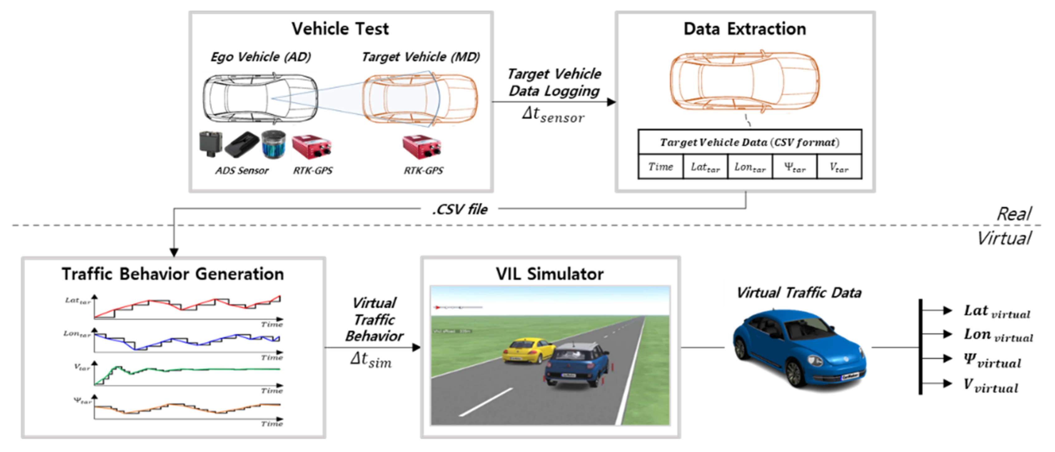
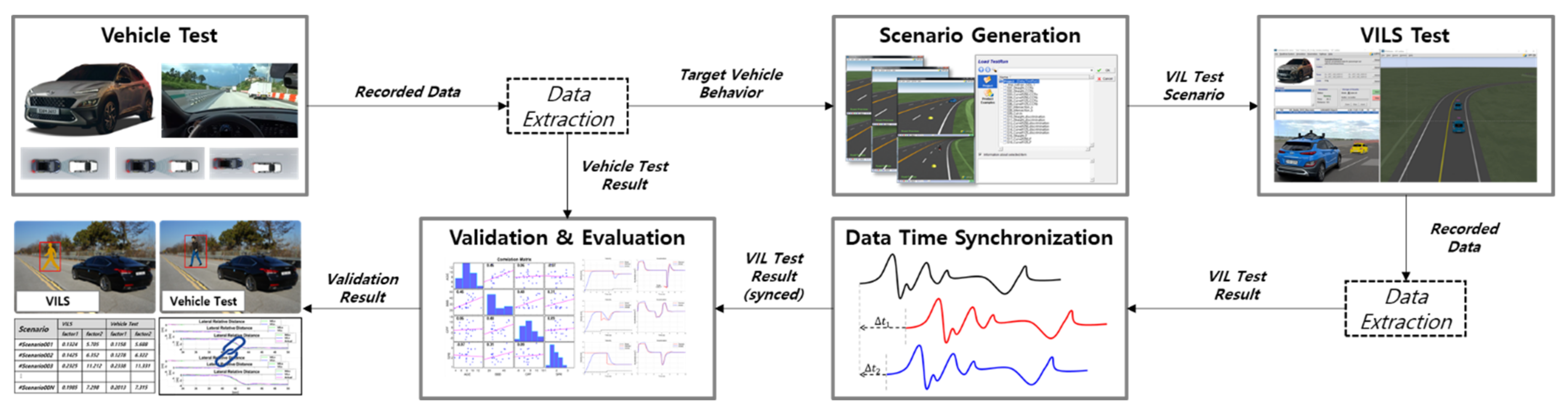
Figure 6 depicts the implementation of the virtual traffic behavior. Firstly, the location, speed, and heading of the RTK-GPS installed in the target vehicle are logged during the vehicle test. The measurement data were logged based on the GPS time provided by the RTK-GPS, and information on the target vehicle was obtained based on the vehicle test time. The location of the target vehicle was measured in terms of latitude and longitude. Therefore, the location of the target vehicle is converted into meter units by performing the UTM conversion, as explained in Section 2.1.

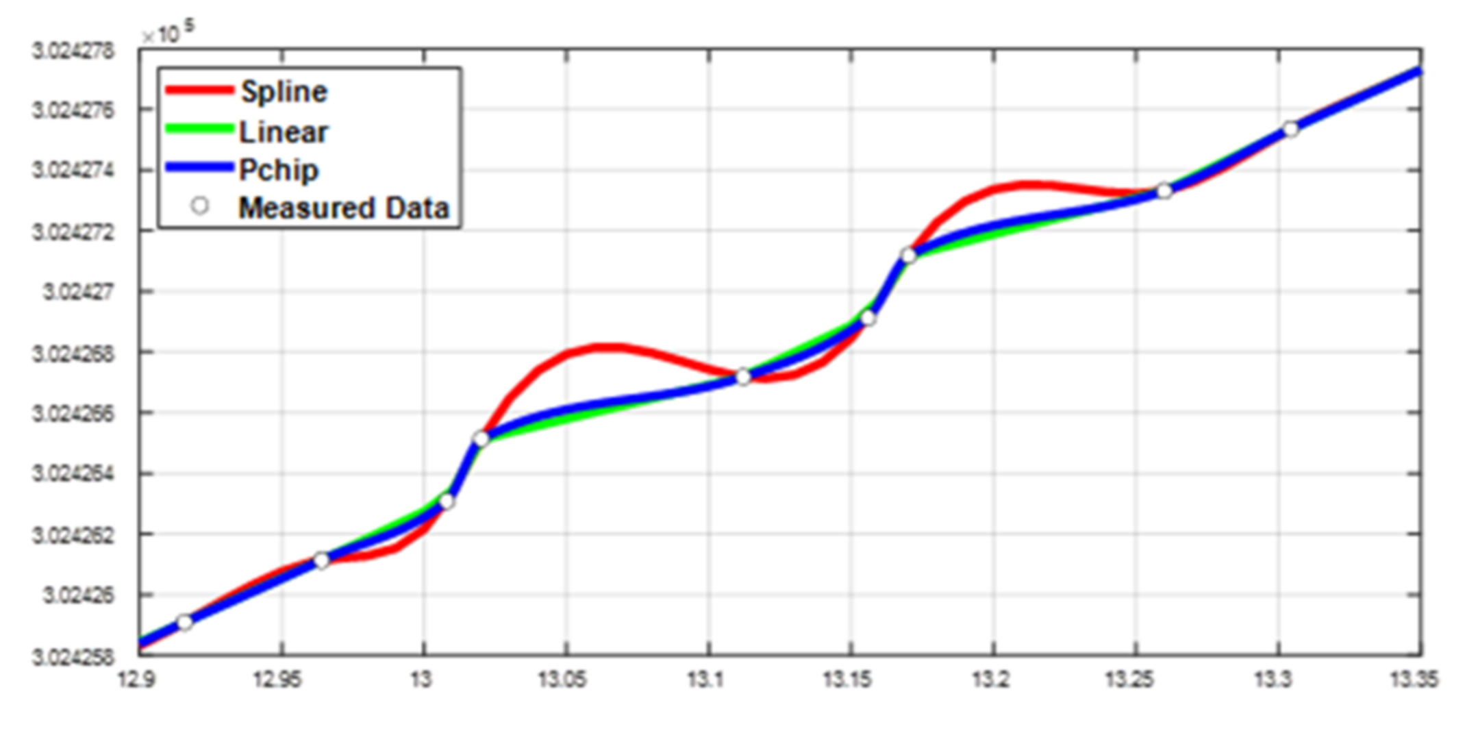
Since the RTK-GPS data of the target vehicle are updated at a frequency lower than that used in the simulation, discontinuous vehicle behavior is observed in the virtual environment. To solve this problem, the logged target vehicle information was interpolated based on the simulation cycle and applied in the virtual simulator. The behavior of the target vehicle was interpolated using the Matlab Interpolation Tool, as shown in Figure 7. The Piecewise Cubic Hermite-Interpolating-Polynomial (PCHIP) method was used for the interpolation; this method interpolates the data most similar to the measured target vehicle data [34,35].

2.4. Perception Sensor Modeling

The virtual traffic implemented as shown above cannot be measured through an actual perception sensor; therefore, a virtual perception sensor model is required to measure this traffic. Perception sensor models can be largely classified as using raw-data or object-list modeling. A raw-data sensor model provides a virtual image or point cloud similar to the real one, and can implement the driving environment in detail. However, it involves a large computational overhead. Conversely, the object-list sensor model can directly provide the data required for vehicle control to reduce the computational overhead and can provide realistic data by replicating physical characteristics such as sensor noise [36,37,38,39]. In this study, the relative distance and speed of the virtual traffic required for the autonomous driving algorithm were generated through object-list-based perception sensor modeling.

The relative distance between the test vehicle and the virtual traffic was determined based on the global location data of the vehicles. If the relative distance is calculated directly through the global location of each vehicle, the generated value is different from the relative distance of the actual perception sensor. This results in a difference in behavior between the vehicle test and the autonomous driving test performed using the VILS, making it difficult to ensure the repeatability and reproducibility.

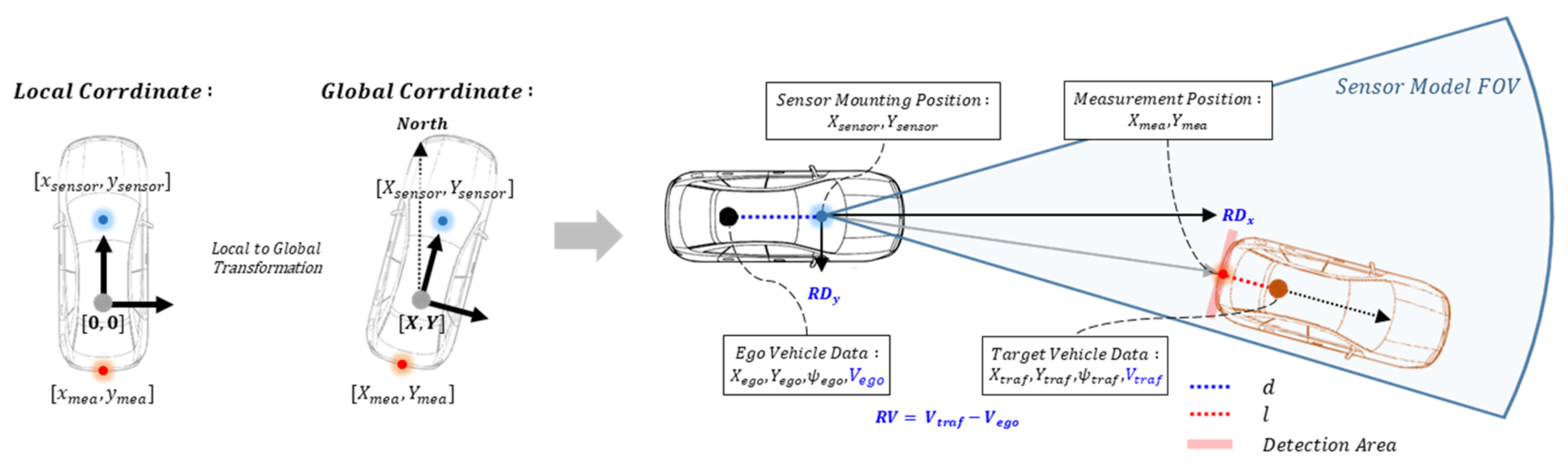
Three aspects must be reflected to generate a value similar to the relative distance of an actual perception sensor. The distance between the test vehicle’s RTK-GPS and the perception sensor mounting point, the RTK-GPS mounting position of the actual target vehicle used to implement the virtual traffic, and the point at which the actual perception sensor detects the target vehicle must be considered. Figure 8 depicts the method used to generate a relative distance which is similar to that of a real perception sensor in the VILS test by considering the aforementioned three factors. The relative distance between the test vehicle and virtual traffic is calculated as follows:

$$\left[\hspace{0.33em}\begin{array}{c}R{D}_x\\ R{D}_y\end{array}\hspace{0.33em}\right]\hspace{0.33em}=\hspace{0.33em}\left[\hspace{0.33em}\begin{array}{c}{X}_{mea}-X_{sensor}\\ Y_{mea}-X_{sensor}\end{array}\hspace{0.33em}\right]\hspace{0.33em}\left[\hspace{0.33em}\begin{array}{cc}\cos (-{\psi }_{ego})& -\sin (-{\psi }_{ego})\\ \sin (-{\psi }_{ego})& \cos (-{\psi }_{ego})\end{array}\hspace{0.33em}\right]$$

(4a)

$$\left[ \begin{array}{c}{X}_{sensor}\\ Y_{sensor}\end{array} \right]=\left[ \begin{array}{c}{d}_x\\ d_y\end{array} \right] \left[ \begin{array}{cc}\cos ({\psi }_{ego})& -\sin ({\psi }_{ego})\\ \sin ({\psi }_{ego})& \cos ({\psi }_{ego})\end{array} \right]+\left[ \begin{array}{c}{X}_{ego}\\ Y_{ego}\end{array} \right]$$

(4b)

$$\left[ \begin{array}{c}{X}_{mea}\\ Y_{mea}\end{array} \right]=\left[ \begin{array}{c}-l_x\\ -l_y\end{array} \right] \left[ \begin{array}{cc}\cos ({\psi }_{traf})& -\sin ({\psi }_{traf})\\ \sin ({\psi }_{traf})& \cos ({\psi }_{traf})\end{array} \right]+\left[\hspace{0.33em}\begin{array}{c}{X}_{traf}\\ Y_{traf}\end{array}\hspace{0.33em}\right]$$

(4c)

Here, the subscripts ${(\hspace{0.33em})}_{sensor}$ and ${(\hspace{0.33em})}_{mea}$ represent the perception sensor mounted on the test vehicle and the point detected by the perception sensor, respectively. The parameter $RD$ represents the relative distance based on the test vehicle; $d$ denotes the distance between the RTK-GPS mounted on the test vehicle and the recognition sensor; and $l$ denotes the distance between the RTK-GPS mounted on the target vehicle and the point detected by the perception sensor of the test vehicle.

The relative speed can be calculated based on the absolute speed difference between the virtual traffic and the test vehicle as shown below:

$$RV=V_{traf}-V_{ego}$$

(4d)

Here, the subscripts ${(\hspace{0.33em})}_{ego}$ and ${(\hspace{0.33em})}_{traf}$ represent each test vehicle and virtual traffic vehicle, $RV$ represents the relative speed, and $V$ represents the vehicle’s absolute speed.

Even if the relative distance and speed of the test vehicle and the virtual traffic are obtained using the above method, the noise component generated by the actual perception sensor cannot be implemented in the virtual environment. Consequently, the RTK-GPS date and perception sensor data which were obtained during the vehicle tests were utilized to implement the sensor noise, which is similar to that of the actual conditions. Firstly, the RTK-GPS-based relative distance and relative speed of the test vehicle and target vehicle measured during the vehicle test were calculated using Equation (4). The error was calculated by comparing the calculated RTK-GPS-based relative distance and speed with the actual perception sensor data, and then calculating the mean and variance of the error using Equations (5a,b). Subsequently, a normal distribution was generated with the mean and variance of the error by using Equation (5c). The relative distance and velocity similar to the actual perception sensor data were generated by inserting the generated normal-distributed noise into the perception sensor model, as follows [40,41,42]:

$$\mu =\frac{1}{n}{\displaystyle \sum _{k=1}^n{X}_k}$$

(5a)

$${\sigma }^2=\frac{{\displaystyle \sum {(X-\mu )}^2}}{n}$$

(5b)

$$N(\mu ,{\sigma }^2)=\frac{1}{\sqrt{2\pi {\sigma }^2}}\times e^{-({(X-\mu )}^2/2{\sigma }^2)}$$

(5c)

Here, $\mu$ denotes the mean of the data, ${\sigma }^2$ denotes the variance, and $n$ denotes the total amount of data. $N(\mu ,{\sigma }^2)$ represents a normal distribution with mean and variance as inputs.

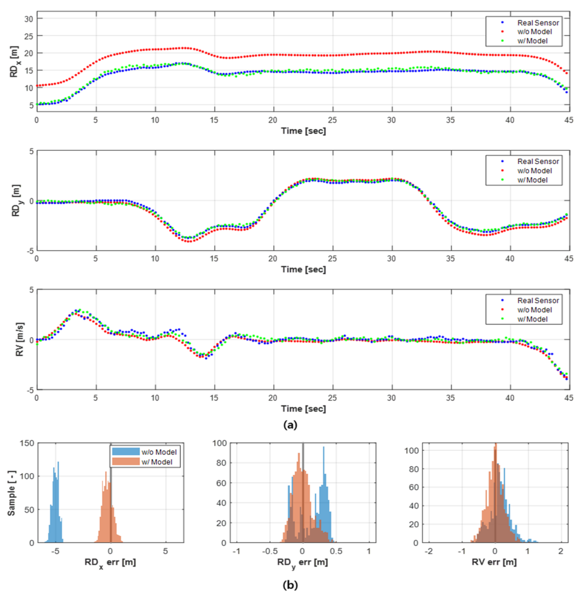
Figure 9a presents the results generated by using the perception sensor modeling process. In the case of the relative distance calculated by using only the RTK-GPS data between each vehicle without sensor modeling (represented by the red point), an error was observed in comparison to the actual recognition sensor data that is sufficient to affect the vehicle control. In the case of the relative distance and speed (represented by the green point) generated through sensor modeling, it can be observed that the trend is similar to the actual perception sensor data (represented by the blue point). Figure 9b presents the distribution of the errors by comparing the data before and after performing sensor modeling using the actual perception sensor data. When sensor modeling is performed, the longitudinal and lateral relative distances and relative speeds present an average error distribution close to 0 when compared to the data obtained before performing sensor modeling.

3. Test Autonomous Driving System

In the VILS, a test vehicle with an autonomous driving function is required to verify the performance, similar to in the vehicle test. The test vehicle comprised an autonomous driving ECU, RTK-GPS equipment, and a control target vehicle. The autonomous driving ECU is used to control the vehicle based on the information obtained in the virtual driving environment, and the real-time performance is verified. The RTK-GPS is used to measure the position, speed, acceleration, and rotation information of the test vehicle. The information obtained in the RTK-GPS is transferred to the synchronization module of the virtual simulator to implement the actual vehicle movement in the virtual environment, as explained in Section 2.2. The vehicle to be controlled is the actual vehicle to which the autonomous driving system is applied, and, in the case of the PG-VILS, the vehicle is driven on a proving ground.

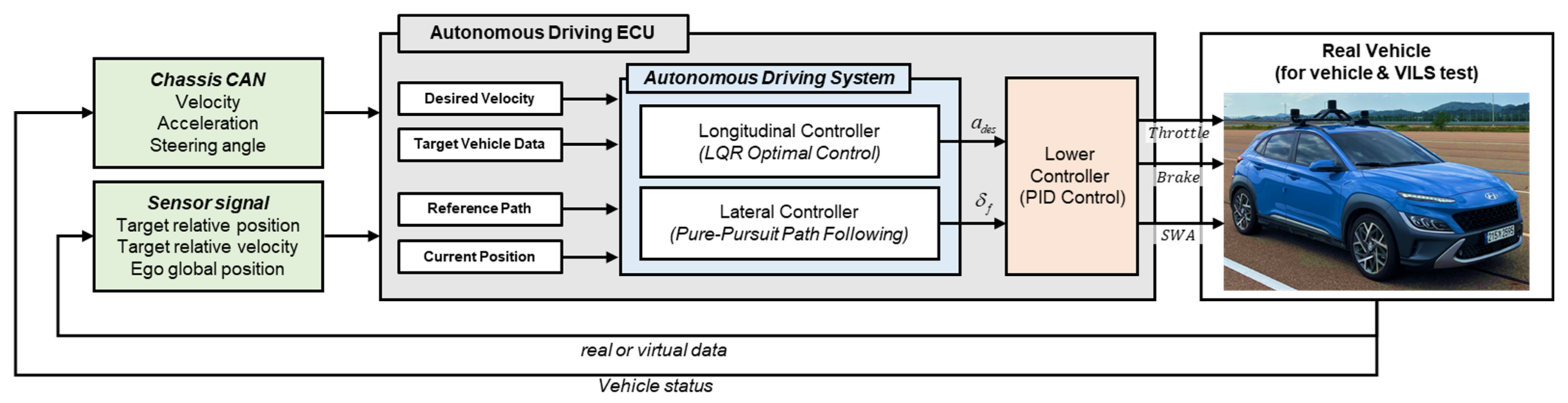
The autonomous driving algorithm for the PG-VILS consists of longitudinal control that maintains the vehicle’s distance from the preceding vehicle and lateral control that follows the designated path. Figure 10 presents the system architecture of the autonomous driving used in this study. In longitudinal control, relative distance and relative speed are used to maintain a distance from a preceding vehicle. In lateral direction control, path-following is performed using global coordinates measured by the RTK-GPS. The output values of the longitudinal and lateral controllers are transferred to the lower controller that controls the actuator of the vehicle. The lower controller uses PID control to generate throttle/brake and steering wheel angle commands for vehicle acceleration/deceleration and steering. Since the lower controller based on PID control has an intuitive and simple structure, a detailed description will be omitted in this paper.

3.1. Longitudinal Controller

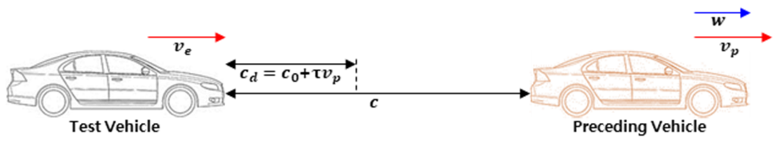
An Adaptive Cruise Control (ACC) system was designed based on LQR optimal control for the longitudinal control. Figure 11 depicts the correlation between the test vehicle and the preceding vehicle in the ACC system, which can be expressed as a state equation, as shown below [43,44]:

$$\dot{x}=Ax+Bu=\left[\begin{array}{cc}0& -1\\ 0& 0\end{array}\right]x+\left[\begin{array}{c}0\\ -1\end{array}\right]u$$

(6a)

$$x=\left[\begin{array}{c}{x}_1\\ x_2\end{array}\right]=\left[\begin{array}{c}{c}_d-c\\ v_p-v_e\end{array}\right]$$

(6b)

Here, $u$ denotes the acceleration of the host vehicle, and $c$ and $c_d$ denote the relative distance and target relative distance to the preceding vehicle, respectively. $v_e$ and $v_p$ represent the speed of the test vehicle and the preceding vehicle, respectively, and $c_0$ represents the safe braking distance. The state variable, $x_1$, represents the error between the target relative distance, $c_d$, and the current relative distance, $c$, and $x_2$ represents the error between the speed of the preceding vehicle and the test vehicle. $c_d$ represents the safe braking distance, time gap, and speed of the preceding vehicle.

To obtain the target acceleration of the test vehicle, a cost function is defined and a control input, $u$, is generated as a value which minimizes it, as shown below:

$$J={\displaystyle {\int }_0^{\infty }(x^{T}Qx+u^{T}Ru)dt}$$

(7)

Here, $Q$ and $R$ represent the weights for the state variable and the input, respectively.

The gain, K, which represents the control input, is calculated using the Ricatti equation as follows:

$$u=a_{des}=-Kx$$

(8a)

$$A^{T}P+PA-PB{R}^{-1}{B}^T+Q=0$$

(8b)

$$K=R^{-1}{B}^{T}P$$

(8c)

Here, $a_{des}$ represents the target acceleration and $P$ represents the solution of the Ricatti equation. In the case of the calculated $a_{des}$, the maximum and minimum values are limited as shown in Equation (9a) to prevent a sudden acceleration/deceleration of the vehicle. When the Time-To-Collision (TTC) (set to 0.8 s in this study) with the preceding vehicle expressed in Equation (9b) lies within the set time, a specific acceleration value is used for emergency braking [45].

$$a_{des}=\left\{\begin{array}{c}{a}_{\max }\\ a_{\min }\\ a_{des}\\ a_{AEB}\end{array}\right.\begin{array}{c}if\\ else\\ else\\ if\end{array}\begin{array}{c} a_{des}>a_{\max }\\ a_{des}<a_{\min }\\ \\ TTC<TT{C}_{\min }\end{array}$$

(9a)

$$TTC=\frac{c}{v_p-v_e}$$

(9b)

Here, $a_{\max }$ and $a_{\min }$ represent the limit values of the required acceleration and $a_{AEB}$ represents the acceleration value used during the emergency braking.

3.2. Lateral Controller

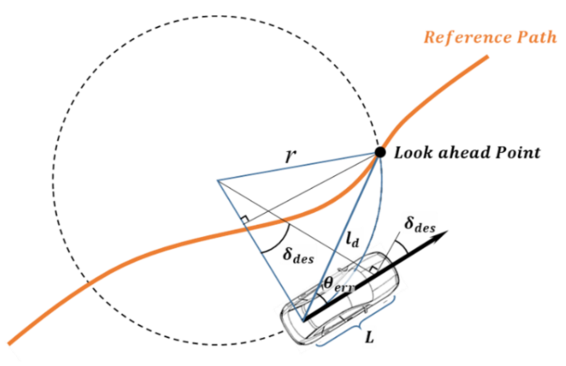
The pure-pursuit algorithm, which is a path-following algorithm, was used for the lateral control [46]. The pure-pursuit algorithm generates the target steering angle to reach the look-ahead point, which is the target point on the path to be followed, as shown in Figure 12. The generated target steering angle is calculated as follows:

$${\delta }_{des}=\frac{L}{r}=\frac{2\sin ({\theta }_{err})}{l_d}\ast L$$

(10a)

$$l_d=v_e\ast k$$

(10b)

Here, $L$ represents the wheelbase of the vehicle, $r$ represents the turning radius, ${\theta }_{err}$ represents the yaw angle between the vehicle heading and the look-ahead point, and $l_d$ represents the distance to the look-ahead point. In the case of $l_d$, the vehicle speed, $v_e$, of the test vehicle and the linear coefficient, $k$, were used in proportion to the vehicle speed. Thus, an appropriate look-ahead point can be determined based on the vehicle speed, while achieving the path-following performance and steering stability.

4. Consistency Validation Procedure and Methodologies

The VILS system must be capable of verifying the autonomous driving system and whether the test results obtained using the proposed VILS are similar to those of the vehicle test. Even if a VILS System with various components has been developed, it is impossible to replicate and reproduce the vehicle test scenario using the VILS system if the behavior of the vehicle is different from that observed during the vehicle test [47].

4.1. Consistency Validation Procedure

Figure 13 depicts the procedure used to verify the consistency between the vehicle test and the VILS test. Firstly, the target vehicle behavior required for the VILS scenario generation and the result data (Control Command, Vehicle Status, etc.) required for consistency verification are extracted from the various pieces of information obtained during the vehicle test. A VILS scenario is then generated using the extracted target vehicle behavior, and the VILS test result data are extracted. Time synchronization is performed based on the Time of Arrival (TOA), which is the time at which the VILS test data reaches a specific value, to compare the results obtained by performing the same VILS scenario several times [48]. The consistency was analyzed and the validity of the proposed VILS system was verified by comparing the time-synchronized VILS test results with the vehicle test results.

4.2. Consistency Validation Methodologies

In this study, a time-series comparison, which quantitatively verifies the consistency of the virtual and real data, and a scalar data comparison, used for data comparison at key points in the test, are utilized [49,50].

In the time-series comparison, NRMSE, which is an index indicating the error between datasets, and the Pearson correlation, which is an index indicating the linear correlation between the two datasets, were used [51]. The NRMSE is a value obtained by dividing the Root Mean Square Error (RMSE) value by the difference between the maximum and minimum data. It can determine the error normalized to a value of 0 to 100, and is expressed as follows [52]:

$$NRMSE=\frac{RMSE}{y_{real,\max }-y_{real,\min }}\times 100=\frac{\sqrt{\frac{1}{N}{\displaystyle {\sum }_i^N{(y_{real,i}-y_{sim,i})}^2}}}{y_{real,\max }-y_{real,\min }}\times 100$$

(11)

Here, $y_{real}$ and $y_{sim}$ represent the real and simulated data, $N$ represents the number of samples of the calculated data, and the subscripts, ${( )}_{\max }$ and ${( )}_{\min }$, represent the maximum and minimum values, respectively.

The Pearson correlation is a value obtained by dividing the absolute value of the covariance of two data points by the product of the standard deviation of each data point. It can be represented as a number between -1 and 1, where a value closer to 1 indicates a higher correlation between the data, and can be expressed as follows [53]:

$$r_{sim,real}=\frac{\left|{\displaystyle {\sum }_i^N(y_{sim,i}-{\overline{y}}_{sim})\times (y_{real,i}-{\overline{y}}_{real})}\right|}{\sqrt{{\displaystyle {\sum }_i^N{(y_{sim,i}-{\overline{y}}_{sim})}^2}\times {\displaystyle {\sum }_i^N{(y_{real,i}-{\overline{y}}_{real})}^2}}}$$

(12)

Here, $r$ denotes the Pearson correlation coefficient, $y_{real}$ and $y_{sim}$ represent the real and simulation data, respectively, and $\overline{y}$ denotes the average of the data, where $N$ indicates the number of samples in the measured data.

In the case of scalar data comparison, the relative error between the virtual and real data is determined as a ratio by comparing the data peak values at a specific point in time. In this study, the peak value of the relative speed which is observed when the preceding vehicle arrives at a sudden stop is compared with the peak value of the longitudinal acceleration of the vehicle performing the AEB. The peak values of the yaw rate/lateral acceleration are obtained when driving on a turning road with a large curvature. The corresponding results are explained in Section 5, and the relative error between the actual and virtual peak data can be expressed as follows [54]:

$$PR=\frac{\left|y_{real,peak}-y_{sim,peak}\right|}{\left|y_{real,peak}\right|}\times 100$$

(13)

Here,$PR$ represents the ratio of the real simulation peak value, $y_{real}$ and $y_{sim}$ represent the real and simulated data, respectively, and the subscript ${( )}_{peak}$ represents the peak value of the data to be compared.

5. Field Test Configuration and Test Result

As explained in the previous section, the consistency of the VILS test results and vehicle test results is an important indicator to ensure that the proposed VILS system can achieve repeatability and reproducibility for a specific scenario. This is because VILS is implemented to replicate scenarios which are difficult to implement repeatedly in a vehicle test through a simulation and to replicate vehicle behaviors with similar tendencies. This section describes the vehicle configuration, test site, and scenario used for the actual vehicle tests and the VILS tests and analyzes the consistency of the test results from the two different environments.

5.1. Experimental Setup

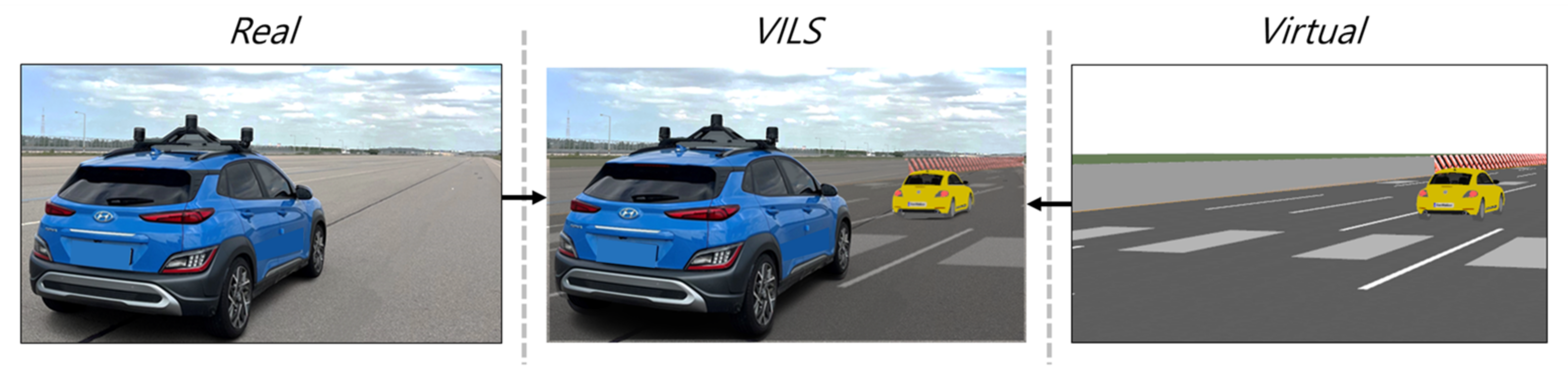
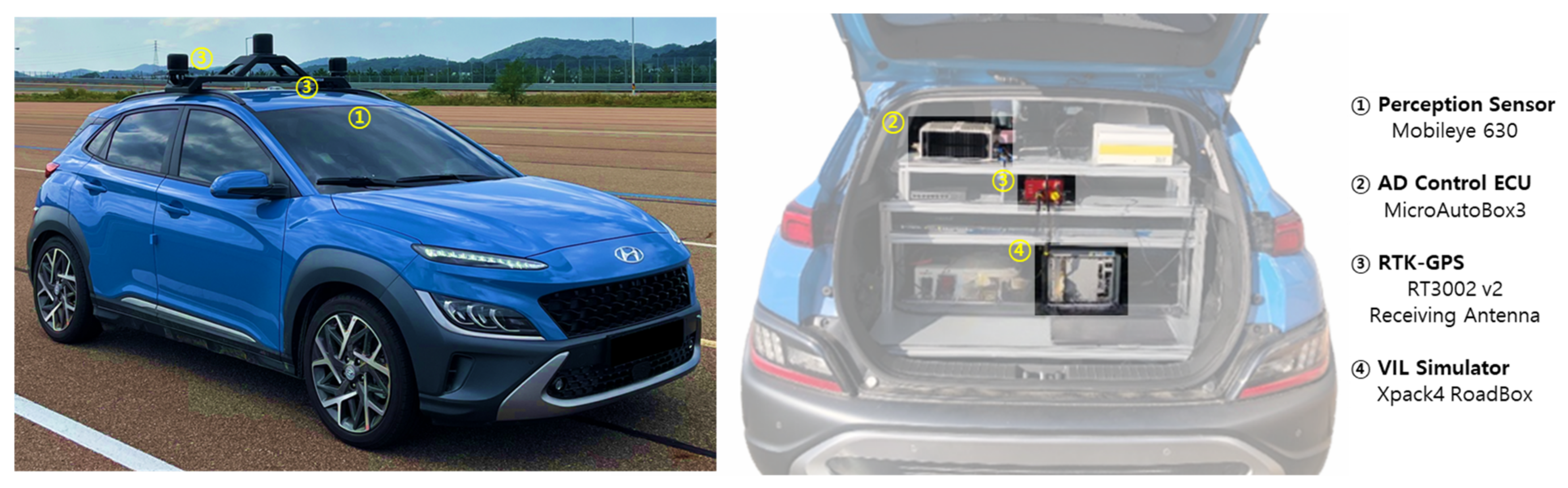
An autonomous vehicle based on the Hyundai Kona was used as the test vehicle, as shown in Figure 14. Mobileye 630 was used as the perception sensor to detect the surrounding vehicles, and a real-time ECU loaded with the autonomous driving algorithm was configured using MicroAutobox3 (MAB3). Additionally, the actual position of the test vehicle was measured using RT3002-v2, and the Xpack4 RoadBox, a real-time computing device, was used as a virtual simulator equipped with the VILS system proposed in this study. In the case of the vehicle test, information on the surrounding vehicles measured in Mobileye and the location information of RT3002-v2 are transmitted to the real-time ECU to perform the longitudinal and lateral control in autonomous driving. In the case of the VILS, the virtual surrounding vehicles and virtual location information generated through the virtual simulator are transmitted to the Real-Time ECU.

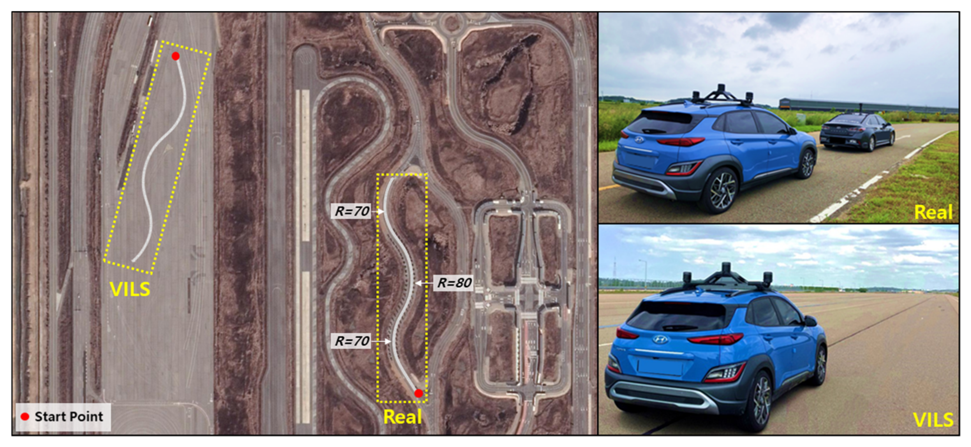
The actual vehicle tests and VILS tests were conducted on the configured test vehicle in K-City (Autonomous Driving Testbed) and on the proving ground located inside the Korea Automobile Testing and Research Institute. The vehicle test was conducted on a suburban road inside K-City, as shown in Figure 15. The driving test was conducted on a selected target road (approximately 320 m in length), which includes curved sections with turning radii of 70 m, 80 m, and 70 m, respectively, among the suburban roads. A test that considered both the longitudinal and lateral dynamics along the target road was conducted. The VILS test was conducted by constructing a virtual road with the same shape as that of the target road selected for the vehicle test. Consequently, some areas within the proving ground that allowed for the target road size were selected for the VILS test.

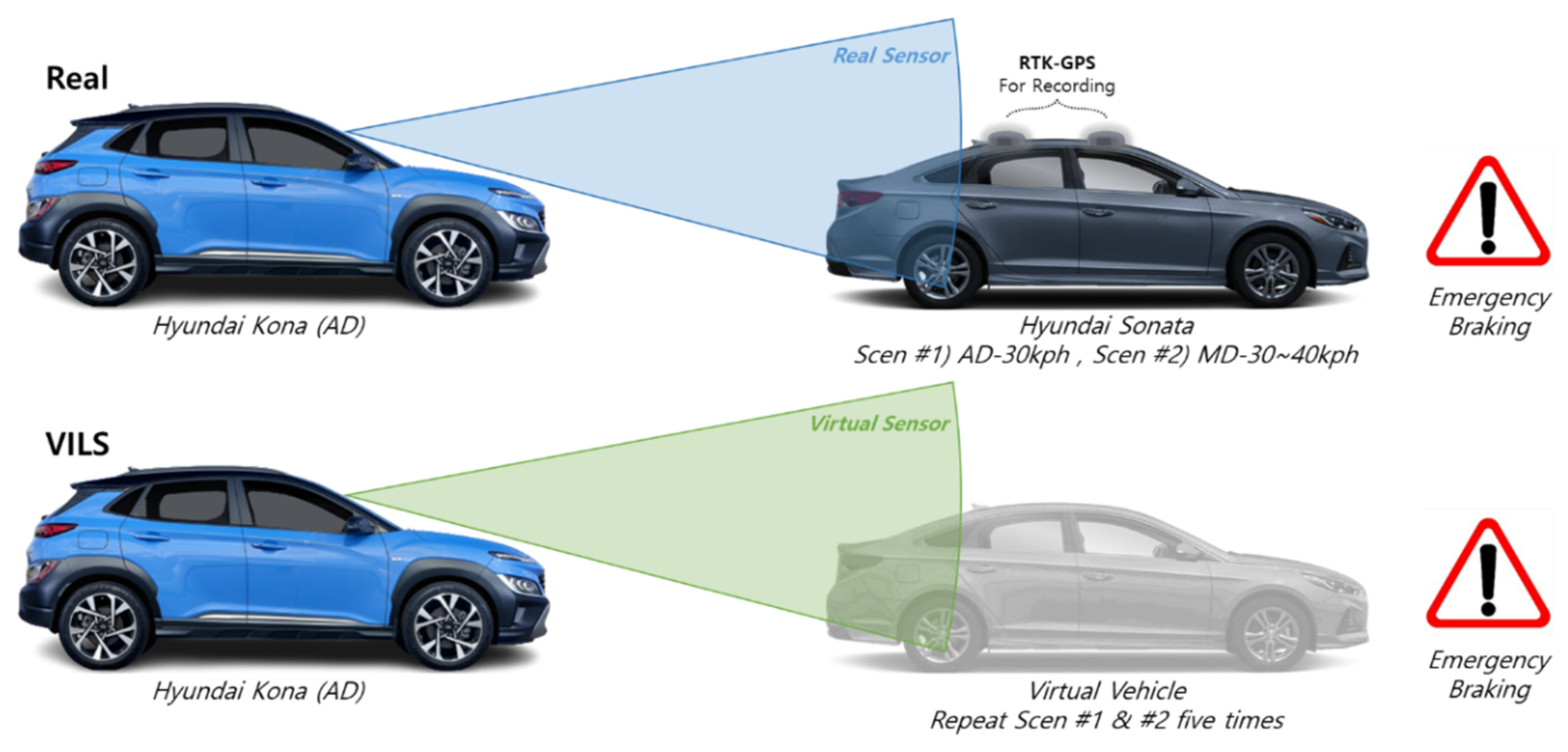
Figure 16 presents the configuration and scenario of the vehicle test conducted using the test vehicle and the target road described above. A Hyundai Sonata was used as the target vehicle, and the ACC function, which maintains a longitudinal distance from the target vehicle, was implemented. The target vehicle was equipped with an autonomous driving function, along with manual driving; it was controlled to follow a set route, and a constant speed was maintained through cruise control. Additionally, it was configured to record the behavior measured using a mounted RTK-GPS. The recorded behavioral information of the target vehicle was used to implement the behavior of the virtual vehicle to be used in the VILS test. The vehicle test scenario was constructed for two cases, one in which the target vehicle was driven autonomously and one manually.

In the first scenario, ACC control is performed on a target vehicle which is driven using autonomous driving to follow a predetermined route. In this scenario, the target vehicle maintains a steady-state speed of 30 km/h and stops when sudden braking is performed at the end of the last curved section (R = 70 m). In the second scenario, longitudinal and lateral control are implemented on a manually driven target vehicle. The vehicle is driven at a speed of 30–40 km/h, and, similarly to in Scenario 1, it is stopped when sudden braking is performed at the end of the last curved section. The speed of the target vehicle in the scenario reflected the width and curvature of the target road to set a safe speed for the test. In addition, in the case of a target vehicle that is manually driven by a real driver, it is difficult to drive the entire section of the target road at a constant speed; therefore, it is driven at a speed within a specific range. The ACC setting for the speed of the test vehicle was set to 50 km/h, which is higher than the driving speed of the target vehicle, in order to respond to the two scenarios.

The vehicle test was conducted using the scenario configured as described above, and the recorded behavior information of the target vehicle was applied to the virtual simulator. The VILS test was performed five times for each scenario, and the consistency of the behavior of the vehicle in the two environments was determined by analyzing the VILS test results and the vehicle test results.

5.2. Test Results

The test results of the two environments were compared by classifying the obtained data into perception sensor data, longitudinal behavior, and lateral behavior, and a Key Performance Index (KPI) was selected for each classification [55]. The KPI of the vehicle test is represented in black, and the KPI of the VILS test, which was performed five times, is represented in five different colors.

The consistency between the vehicle test and the VILS test was analyzed based on the results of each KPI. The NRMSE, Pearson correlation, and peak-ratio comparison methods, which were explained in Section 4, were used for the consistency analysis. The NRMSE is an index that indicates the error between datasets, and the Pearson correlation is an index that indicates a linear correlation between two datasets. The peak-ratio comparison is an indicator to determine whether the data peak values observed at a specific point in time, such as during emergency braking, are similar to each other in the vehicle test and VILS test.

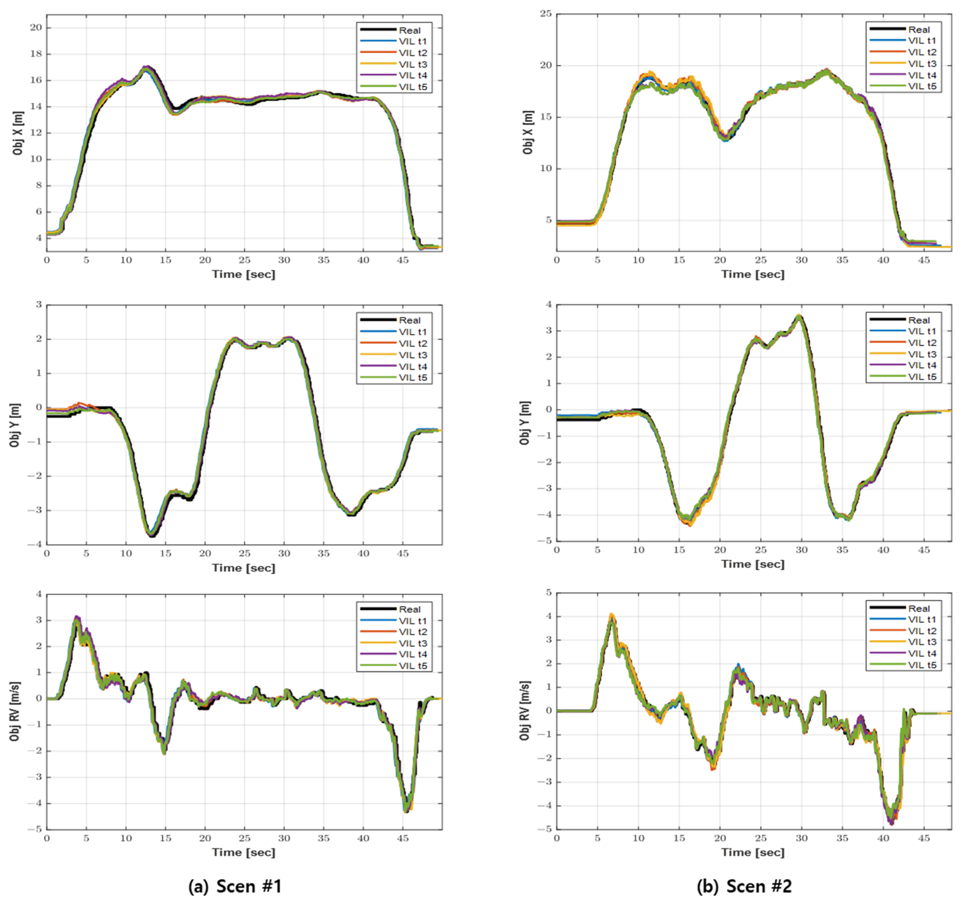
5.2.1. Test Result #1—Sensor Data

In this section, the validity of the proposed sensor model of the VILS system is verified by analyzing the consistency between the virtual perception sensor data generated during the VILS and the actual sensor perception data. First, the longitudinal/lateral relative distance and relative speed of the target object, which are the sensor data necessary for the ACC performed by the test vehicle, were selected as the KPIs of the sensor data. To ensure high consistency with the vehicle test, the generated virtual perception sensor data of the VILS System must be similar to the vehicle test data. This is because, when the generated virtual perception sensor data are not similar to the real data, the control command value generated by the autonomous driving algorithm may exhibit a completely different behavior.

Figure 17a depicts Scenario 1 and Figure 17b depicts Scenario 2. In Scenario 1, the front target vehicle is autonomously driven at a fixed speed. Therefore, it exhibits a constant trend in the relative distance and relative speed after the steady state. In Scenario 2, the measured sensor data values are not constant when compared to those of Scenario 1 since the front target vehicle is manually driven.

The five VILS tests performed using these scenarios demonstrated that the results of the VILS tests were similar to the sensor information obtained during the vehicle test, as shown in Figure 17. A comparison of the errors of each VILS test and the vehicle test demonstrated that the NRMSE of the longitudinal/lateral relative distance and the relative speed presented an average value of approximately two percent, as shown in

Table 2. Data comparison result—Sensor data (Object relative distance, Object relative velocity) KPI.

Real—VILS (Scen #1)	NRMSE [%]			Pearson Correlation
	ObjX	ObjY	ObjRV	ObjX	ObjY	ObjRV
#1	2.13	2.41	2.71	0.99	0.99	0.98
#2	1.76	1.87	2.07	0.99	0.99	0.99
#3	1.98	2.28	2.68	0.99	0.99	0.99
#4	1.84	1.24	1.68	0.99	0.99	0.99
#5	1.60	1.80	2.30	0.99	0.99	0.99
Avg	1.80	1.80	2.18	0.99	0.99	0.99
Real—VILS (Scen #2)	NRMSE [%]			Pearson Correlation
	ObjX	ObjY	ObjRV	ObjX	ObjY	ObjRV
#1	1.61	1.48	1.97	0.99	0.99	0.99
#2	1.56	0.99	1.33	0.99	0.99	0.99
#3	2.18	1.21	1.87	0.99	0.99	0.99
#4	2.04	1.34	2.30	0.99	0.99	0.99
#5	2.17	1.61	2.91	0.99	0.99	0.99
Avg	1.99	1.29	2.10	0.99	0.99	0.99

. Even in the case of the Pearson correlation, it can be observed that the VILS system, which was built with a high positive correlation close to one, generates sensor data similar to those of the practical conditions.

Table 3. Data Comparison Result—Object relative velocity Peak-Ratio.

Real—VILS (Scen #1)	$\mathit{P}\mathit{R} [\%]$	Real—VILS (Scen #2)	$\mathit{P}\mathit{R} [\%]$
	Obj RV		Obj RV
#1	0.70	#1	1.89
#2	0.46	#2	1.05
#3	2.32	#3	0.42
#4	2.55	#4	0.63
#5	0.23	#5	4.42
Avg	1.25	Avg	1.68

presents the comparison results of the relative speed of the front target vehicle, which was measured during the sudden braking at the end of the target road. This relative speed has an error rate of less than 2.5% on average when compared to the vehicle test in both scenarios. This comparison confirmed the validity of the virtual perception sensor data generated by the proposed VILS system.

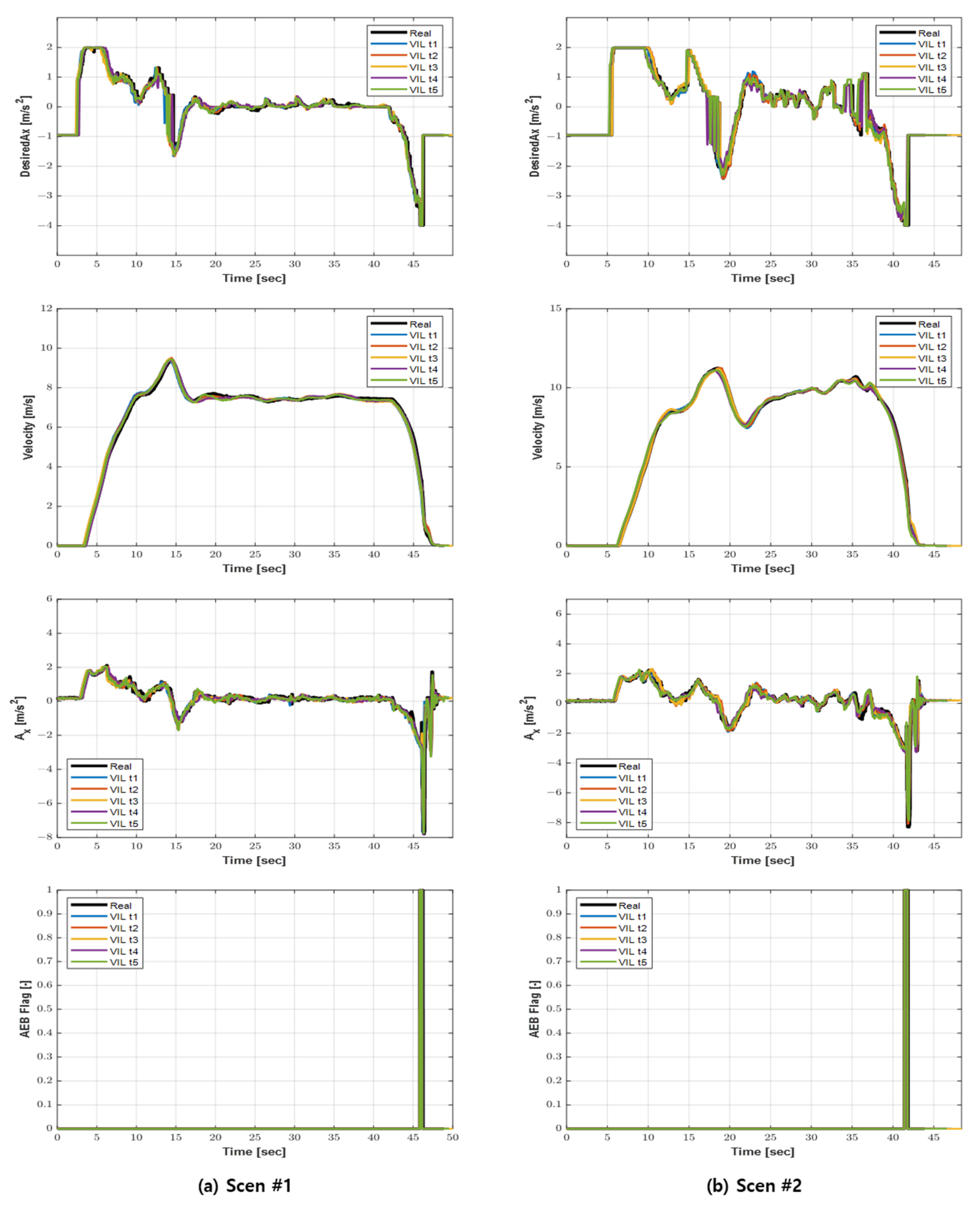
5.2.2. Test Result #2—Longitudinal Behavior (Adaptive Cruise Control)

In this section, the longitudinal behavior consistency of the vehicle test and VILS test is analyzed. The desired acceleration, velocity, longitudinal acceleration, and AEB flag were selected as the KPIs corresponding to the longitudinal behavior, and a consistency analysis was conducted. Figure 18 depicts the longitudinal behavior of the KPIs for the two selected scenarios. In the case of Scenario 1, it can be observed that the values of the speed, longitudinal acceleration, and required acceleration of the test vehicle are constant, except for the acceleration section, since the front target vehicle drove the target road at a constant speed. In Scenario 2, the test vehicle controls the front target vehicle, which is manually driven, and the required acceleration value, which is the control command value, is not uniformly generated, unlike in Scenario 1. Therefore, the vehicle speed is maintained at a value between approximately 30 km/h and 40 km/h (approximately 8 to 11 m/s), and the longitudinal acceleration value also changes based on the required acceleration value.

In both scenarios, the front target vehicle performs sudden braking at the endpoint of the driving target road; the test vehicle also implements control to activate the AEB. If the set TTC condition is not satisfied, the autonomous driving controller outputs an AEB Flag signal even though the minimum required acceleration calculated by the autonomous driving controller of $-4{\mathrm{m}/\mathrm{s}}^2$ is applied to the vehicle. Simultaneously, the acceleration command ($-8{\mathrm{m}/\mathrm{s}}^2$) required for sudden braking is input to the vehicle actuator.

The five VILS tests performed using these scenarios demonstrated that they were implemented in a similar manner to the longitudinal behavior information obtained during the vehicle test.

The NRMSE for the longitudinal KPIs was within four percent on average, and the Pearson correlation exhibited a positive correlation close to one, as shown in

Table 4. Data Comparison Result—Longitudinal behavior (Desired longitudinal acceleration, Velocity and Longitudinal acceleration) KPI.

Real—VILS (Scen #1)	NRMSE [%]			Pearson Correlation
	Desired_Ax	Vel	Ax	Desired_Ax	Vel	Ax
#1	4.21	2.08	4.34	0.95	0.99	0.88
#2	5.71	1.16	3.23	0.97	0.99	0.93
#3	3.98	1.96	3.15	0.96	0.99	0.94
#4	3.04	0.31	2.26	0.98	0.99	0.97
#5	2.33	1.29	2.82	0.97	0.99	0.95
Avg	3.76	1.18	2.87	0.966	0.99	0.934
Real—VILS (Scen #2)	NRMSE [%]			Pearson Correlation
	Desired_Ax	Vel	Ax	Desired_Ax	Vel	Ax
#1	2.49	1.13	3.34	0.97	0.99	0.95
#2	1.79	0.72	2.08	0.98	0.99	0.98
#3	2.40	1.18	3.86	0.97	0.99	0.94
#4	2.95	1.74	3.58	0.95	0.99	0.95
#5	2.70	0.60	4.21	0.96	0.99	0.93
Avg	2.46	1.06	3.43	0.966	0.99	0.95

. The AEB flag was also observed at a similar time to the time observed during the vehicle test, confirming the repeatability of the scenario in which the same emergency braking situation occurs at the same location and at the same time. Additionally, the longitudinal acceleration peak values in the vehicle test and VILS test, which occur in the AEB situation near the test endpoint, were compared as shown in

Table 5. Data Comparison Result—Longitudinal acceleration Peak-Ratio.

Real—VILS (Scen #1)	$\mathit{P}\mathit{R} [\%]$	Real—VILS (Scen #2)	$\mathit{P}\mathit{R} [\%]$
	Ax		Ax
#1	7.18	#1	3.25
#2	5.00	#2	3.37
#3	6.28	#3	2.53
#4	6.28	#4	5.66
#5	6.15	#5	0.48
Avg	6.18	Avg	3.06

. The comparison results demonstrate that, in Scenario 1, the average error rate was 6.18%, and, in Scenario 2, the average error rate was 3.06%. As the test vehicle was driven on a real proving ground instead of a virtual one, the VILS test result exhibits some error every time. However, since the error in each test is not at a level that exhibits a different trend from the vehicle test, the validity of the longitudinal control test performed using the proposed VILS system is demonstrated.

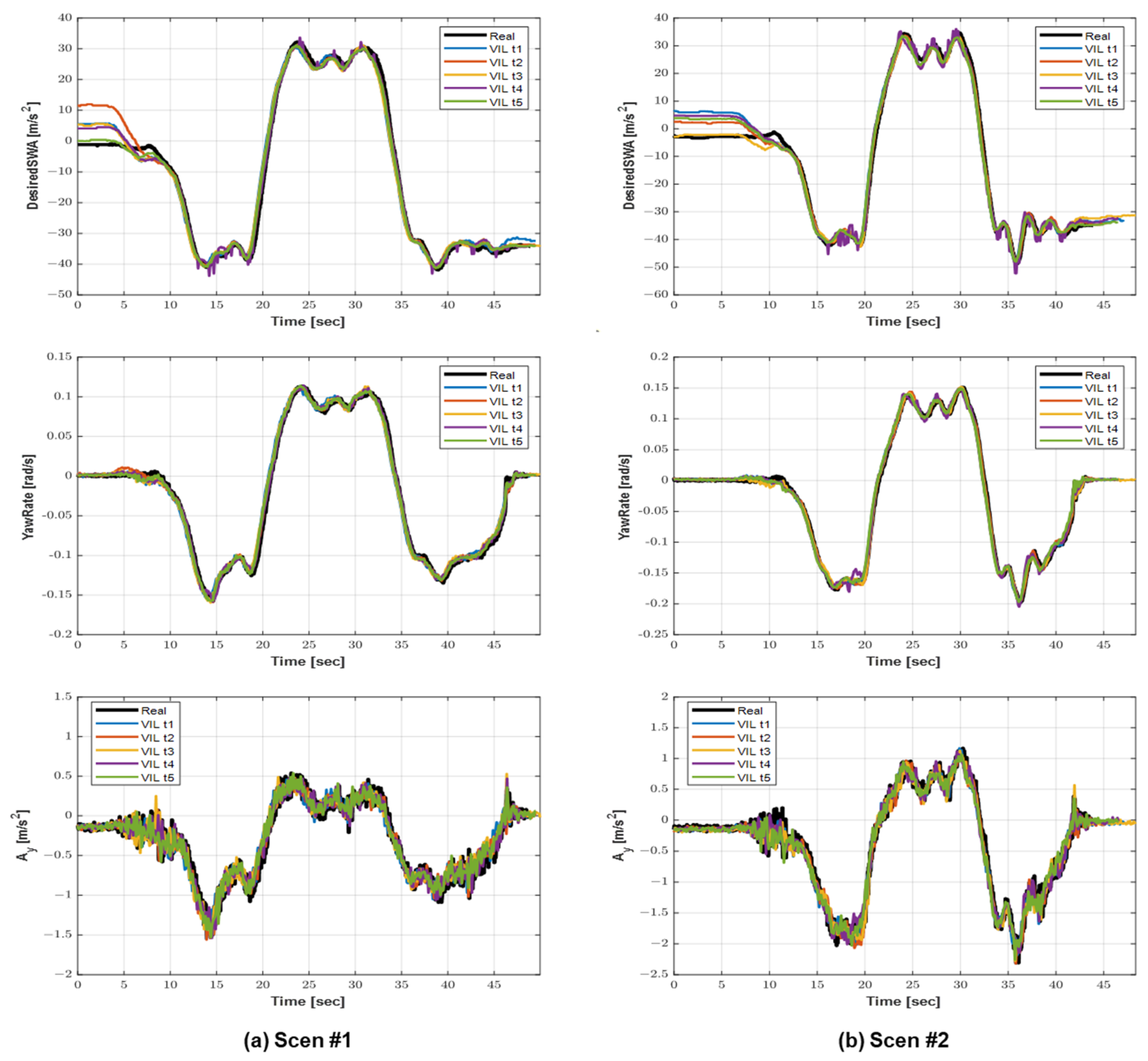
5.2.3. Test Result #3—Lateral Behavior (Path Following)

The consistency of the lateral behavior of the test vehicle and the VILS test was analyzed by selecting the desired Steering Wheel Angle (SWA), yaw rate, and lateral acceleration as the related KPIs. In both scenarios described above, the test vehicle is driven in a three-section curved road (radius of curvature = 70 m, 80 m, and 70 m) on the target road through path-following control. Figure 19 presents the lateral KPI data of the vehicle test and VILS test conducted based on this scenario. The desired SWA is generated to travel on a set route, and the yaw rate and lateral acceleration generated as a result are presented. It can be observed that, for the desired SWA, the initial values of the vehicle and VILS tests are different. This error is attributed to the fact that the SWA arranged at the start of the test was different for each VILS test. When the test vehicle is driven using the autonomous driving algorithm, the desired SWA is generated in a manner similar to the vehicle test. It can be observed that the yaw rate and lateral acceleration also appear to be similar to the results of the vehicle test.

The NRMSE for the lateral KPIs was within 5.5% on average, and the Pearson correlation also exhibited a positive correlation close to 1, as shown in

Table 6. Data Comparison Result—Lateral behavior (Desired steering wheel angle, Yaw rate, Lateral acceleration) KPI.

Real—VILS (Scen #1)	NRMSE [%]			Pearson Correlation
	Desired_SWA	YawRate	Ay	Desired_SWA	YawRate	Ay
#1	4.21	2.92	5.56	0.99	0.99	0.97
#2	5.71	1.78	5.03	0.99	0.99	0.97
#3	3.98	2.73	5.91	0.99	0.99	0.96
#4	3.04	1.6	5.24	0.99	0.99	0.97
#5	2.33	2.05	5.27	0.99	0.99	0.97
Avg	3.76	2.04	5.36	0.99	0.99	0.97
Real—VILS (Scen #2)	NRMSE [%]			Pearson Correlation
	Desired_SWA	YawRate	Ay	Desired_SWA	YawRate	Ay
#1	4.88	1.6	3.57	0.99	0.99	0.99
#2	3	1.04	2.93	0.99	0.99	0.99
#3	2.13	1.39	3.45	0.99	0.99	0.99
#4	4.58	2.19	3.98	0.99	0.99	0.99
#5	3.86	2.23	3.95	0.99	0.99	0.99
Avg	3.39	1.71	3.58	0.99	0.99	0.99

. However, it presents a higher NRMSE value than the sensor data KPI and longitudinal KPI. This is caused by the SWA of the initially aligned test vehicle, and, after the test vehicle starts driving, it does not cause a significant difference in the vehicle behavior from the vehicle test, as explained above. The yaw rate and lateral acceleration values generated when turning in a curved line were used for the comparison of the peak values. In Scenario 1, the peak value was observed on the first curved road (radius of curvature = 70 m) because this curved section was encountered when the test vehicle started driving and accelerated. In Scenario 2, the acceleration of the test vehicle occurred on the third curved road (radius of curvature = 70 m), resulting in a peak value. The peak ratio of each scenario was compared, and it was observed that the yaw rate ratios were 1.04% and 1.17%, and the lateral acceleration ratios were 3.31% and 2.25%, respectively, as shown in

Table 7. Data comparison result—Yaw rate, Lateral acceleration Peak-Ratio.

Real—VILS (Scen #1)	$\mathit{P}\mathit{R} [ \% ]$		Real—VILS (Scen #2)	$\mathit{P}\mathit{R} [ \% ]$
	YawRate	Ay		YawRate	Ay
#1	0.33	2.65	#1	0.44	0.43
#2	1.77	3.31	#2	0.18	1.73
#3	1.33	5.30	#3	0.26	1.30
#4	1.11	2.65	#4	4.50	5.63
#5	0.66	2.65	#5	0.44	2.16
Avg	1.04	3.31	Avg	1.17	2.25

. In both scenarios, the peak value of the VILS test was observed to be similar to that of the vehicle test. The above results demonstrate the validity of the lateral control test performed using the proposed VILS system.

6. Conclusions

In this study, a VILS system which considers the consistency between the vehicle test and VILS test results was proposed. Four components of the VILS system were implemented to obtain simulation results similar to the behavior of a vehicle during vehicle testing. First, a virtual road was built, and the behavior of the test vehicle in the real environment and the virtual environment were synchronized. In addition, the behavior of the surrounding traffic measured during the vehicle test was implemented in the simulation. Finally, a virtual perception sensor that outputs similar values to the real perception sensor was modeled. The VILS test was conducted using the VILS system built through the above process.

The VILS test results and vehicle test results were analyzed using three types of coherence measures (i.e., NRMSE, Pearson correlation, data peak value comparison), which verified that the vehicle behavior in the two different environments was similar. In particular, as the peak values of the two environments show a small difference of around five percent, it can be seen that the vehicle behavior at a specific point is similarly repeated and reproduced. Furthermore, it was verified that the proposed VILS system can simulate not only general driving situations, but also dangerous driving situations, by applying a scenario in which the target vehicle behavior changes between autonomous driving and manual driving.

In the near future, the proposed VILS system will be expanded to be applied to various speeds, road types, and surrounding environments. Additionally, the proposed VILS system can be improved through virtual perception sensor advancement, which considers the characteristics and modeling methodologies of various perception sensors. With these improvements, the VILS system is expected to be able to verify various autonomous driving functions in addition to the ACC and path-following functions.