
Three-Stage Tone Mapping Algorithm


Abstract
1. Introduction
2. Related Work
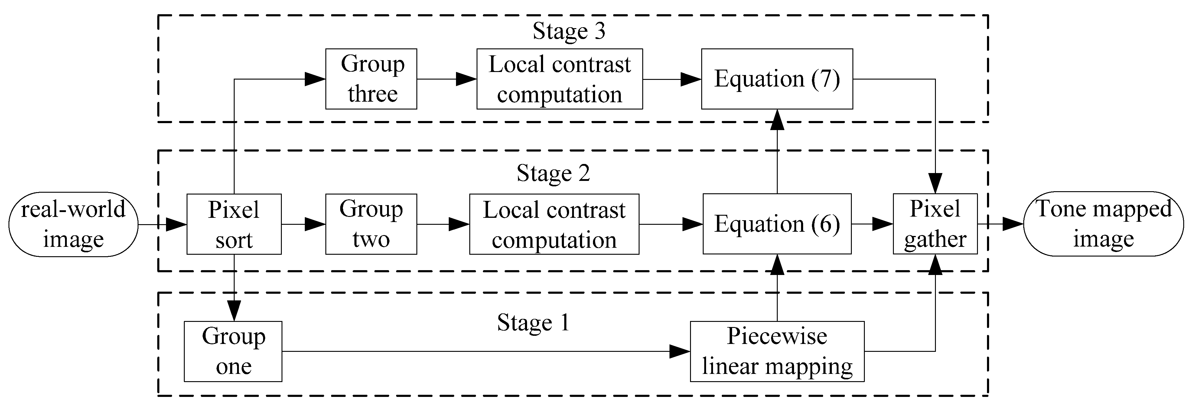
3. Algorithm
3.1. Global Luminance Mapping
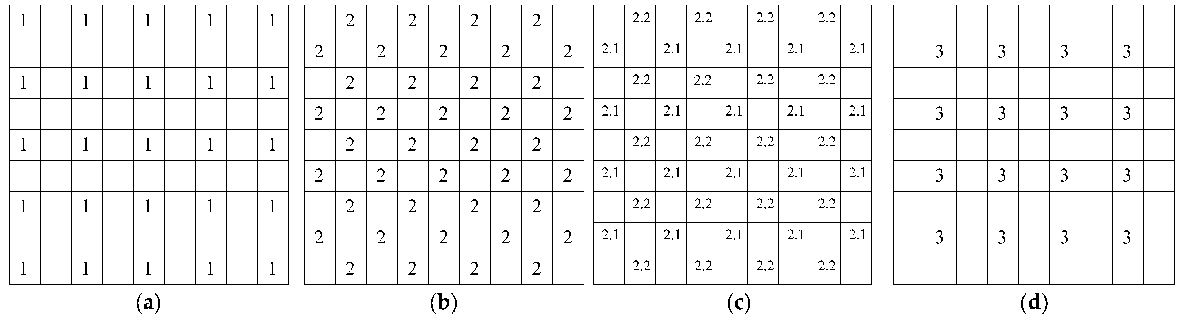
3.2. Local Contrast Preservation
3.3. Color Image
4. Results
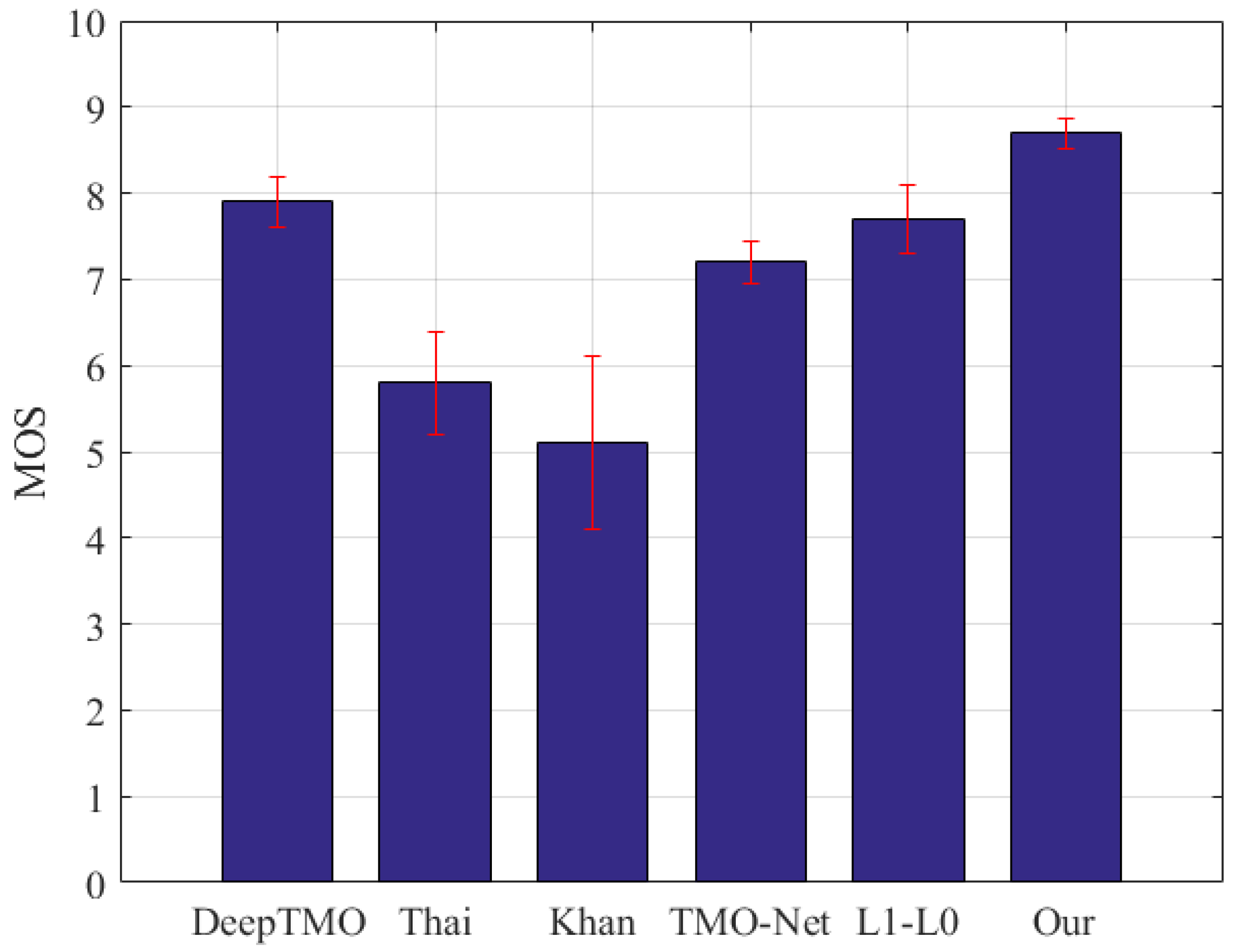
4.1. Subjective Performance Evaluation
4.2. Objective Performance Evaluation
4.3. Hardware Platform Test
5. Conclusions
Author Contributions
Funding
Acknowledgments
Conflicts of Interest
References
- Kalantari, N.K.; Ramamoorthi, R. Deep high dynamic range imaging of dynamic scenes. ACM Trans. Graph. 2017, 36, 144. [Google Scholar] [CrossRef]
- Ou, Y.; Ambalathankandy, P.; Takamaeda, S.; Motomura, M.; Asai, T.; Ikebe, M. Real-time tone mapping: A survey and cross-implementation hardware benchmark. IEEE Trans. Circuits Syst. Video Technol. 2022, 32, 2666–2686. [Google Scholar] [CrossRef]
- Yue, G.; Yan, W.; Zhou, T. Referenceless quality evaluation of tone-mapped HDR and multiexposure fused images. IEEE Trans. Ind. Inform. 2019, 16, 1764–1775. [Google Scholar] [CrossRef]
- Jiang, M.; Shen, L.; Hu, M.; An, P.; Gu, Y.; Ren, F. Quantitative measurement of perceptual attributes and artifacts for tone-mapped HDR display. IEEE Trans. Instrum. Meas. 2022, 71, 1–11. [Google Scholar] [CrossRef]
- Fattal, R.; Lischinski, D.; Werman, M. Gradient domain high dynamic range compression. In Proceedings of the 29th Annual Conference on Computer Graphics and Interactive Techniques, New York, NY, USA, 23–26 July 2002. [Google Scholar]
- Eilertsen, G.; Mantiuk, R.K.; Unger, J. A comparative review of tone-mapping algorithms for high dynamic range video. Comput. Graph. Forum 2017, 36, 565–592. [Google Scholar] [CrossRef]
- Ashikhmin, M. A tone mapping algorithm for high contrast images. In Proceedings of the Eurographics Workshop on Rendering, Pisa, Italy, 26–28 June 2002. [Google Scholar]
- Zai, G.J.; Liu, Y. An improved tone mapping algorithm for high dynamic range images. In Proceedings of the International Conference on Computer Application and System Modeling, Taiyuan, China, 22–24 October 2010. [Google Scholar]
- Tumblin, J.; Rushmeier, H. Tone reproduction for realistic images. IEEE Comput. Graph. Appl. 1993, 13, 42–48. [Google Scholar] [CrossRef]
- Ward, G. A contrast-based scalefactor for luminance display. Graph. Gems 1994, 4, 415–421. [Google Scholar]
- Larson, G.W.; Rushmeier, H.; Piatko, C. A visibility matching tone reproduction operator for high dynamic range scenes. IEEE Trans. Vis. Comput. Graph. 1997, 3, 291–306. [Google Scholar] [CrossRef]
- Khan, I.R.; Aziz, W.; Shim, S.O. Tone-mapping using perceptual-quantizer and image histogram. IEEE Access 2020, 8, 31350–31358. [Google Scholar] [CrossRef]
- Meylan, L.; Süsstrunk, S. High dynamic range image rendering using a retinex-based adaptive filter. IEEE Trans. Image Process. 2006, 15, 2820–2830. [Google Scholar] [CrossRef] [PubMed]
- Gu, B.; Li, W.; Zhu, M.; Wang, M. Local edge-preserving multiscale decomposition for high dynamic range image tone mapping. IEEE Trans. Image Process. 2012, 22, 70–79. [Google Scholar] [PubMed]
- Kuang, J.; Johnson, G.M.; Fairchild, M.D. iCAM06: A refined image appearance model for HDR image rendering. J. Vis. Commun. Image Represent. 2007, 18, 406–414. [Google Scholar] [CrossRef]
- Rana, A.; Singh, P.; Valenzise, G.; Dufaux, F.; Komodakis, N.; Smolic, A. Deep tone mapping operator for high dynamic range images. IEEE Trans. Image Process. 2019, 29, 1285–1298. [Google Scholar] [CrossRef] [PubMed]
- Panetta, K.; Kezebou, L.; Oludare, V.; Agaian, S.; Xia, Z. TMO-Net: A parameter-free tone mapping operator using generative adversarial network, and performance benchmarking on large scale HDR dataset. IEEE Access 2021, 9, 39500–39517. [Google Scholar] [CrossRef]
- Patel, V.A.; Shah, P.; Raman, S. A generative adversarial network for tone mapping hdr images. In Proceedings of the National Conference on Computer Vision, Pattern Recognition, Image Processing, and Graphics, Mandi, India, 16–19 December 2017. [Google Scholar]
- Yeganeh, H.; Wang, Z. Objective quality assessment of tone-mapped images. IEEE Trans. Image Process. 2012, 22, 657–667. [Google Scholar] [CrossRef] [PubMed]
- Reinhard, E.; Stark, M.; Shirley, P.; Ferwerda, J. Photographic tone reproduction for digital images. ACM Trans. Graph. 2002, 22, 267–276. [Google Scholar] [CrossRef]
- Reinhard, E. Parameter estimation for photographic tone reproduction. J. Graph. Tools 2002, 7, 45–51. [Google Scholar] [CrossRef]
- Thai, B.C.; Mokraoui, A.; Matei, B. Contrast enhancement and details preservation of tone mapped high dynamic range image. J. Vis. Commun. Image Represent. 2019, 58, 589–599. [Google Scholar] [CrossRef]
- Liang, Z.; Xu, J.; Zhang, D.; Cao, Z.; Zhang, L. A hybrid l1-l0 layer decomposition model for tone mapping. In Proceedings of the IEEE Conference on Computer Vision and Pattern Recognition, Salt Lake City, UT, USA, 18–23 June 2018. [Google Scholar]
- Narwaria, M.; Da Silva, M.P.; Le Callet, P.; Pépion, R. Tone mapping based HDR compression: Does it affect visual experience? Signal Process. Image Commun. 2014, 29, 257–273. [Google Scholar] [CrossRef]
- Mittal, A.; Soundararajan, R.; Bovik, A.C. Making a “completely blind” image quality analyzer. IEEE Signal Process. Lett. 2012, 20, 209–212. [Google Scholar] [CrossRef]


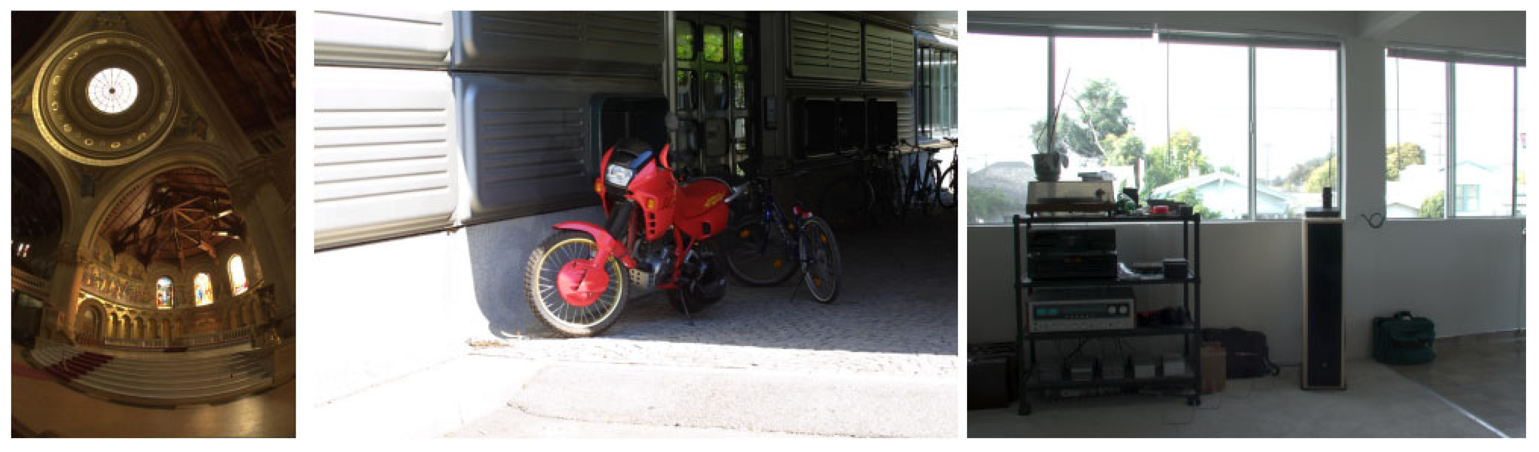
| Algorithm | Memorial Church | Moto | Apartment | |||
|---|---|---|---|---|---|---|
| TMQI | NIQE | TMQI | NIQE | TMQI | NIQE | |
| L1-L0 | 0.893 | 3.62 | 0.876 | 3.73 | 0.834 | 3.82 |
| DeepTMO | 0.905 | 3.35 | 0.904 | 3.59 | 0.798 | 3.31 |
| Khan | 0.652 | 5.29 | 0.622 | 6.21 | 0.649 | 5.45 |
| TMO-Net | 0.852 | 4.28 | 0.814 | 5.07 | 0.824 | 4.34 |
| Thai | 0.711 | 6.67 | 0.685 | 6.75 | 0.659 | 5.75 |
| Our | 0.929 | 3.21 | 0.919 | 3.42 | 0.854 | 3.03 |
| Image Index | DeepTMO | Thai | TMO-Net | L1-L0 | Khan | Our | ||||||
|---|---|---|---|---|---|---|---|---|---|---|---|---|
| TMQI | NIQE | TMQI | NIQE | TMQI | NIQE | TMQI | NIQE | TMQI | NIQE | TMQI | NIQE | |
| 1 | 0.801 | 3.21 | 0.733 | 6.66 | 0.810 | 3.60 | 0.850 | 3.15 | 0.788 | 5.35 | 0.900 | 3.11 |
| 2 | 0.829 | 3.24 | 0.701 | 5.65 | 0.844 | 3.97 | 0.796 | 3.13 | 0.553 | 5.82 | 0.888 | 3.06 |
| 3 | 0.843 | 3.87 | 0.710 | 5.69 | 0.875 | 4.14 | 0.879 | 3.81 | 0.654 | 5.93 | 0.891 | 3.32 |
| 4 | 0.885 | 3.84 | 0.671 | 5.82 | 0.854 | 4.33 | 0.863 | 3.58 | 0.721 | 6.36 | 0.897 | 3.46 |
| 5 | 0.812 | 3.84 | 0.681 | 4.75 | 0.760 | 4.47 | 0.837 | 3.57 | 0.619 | 5.53 | 0.904 | 3.47 |
| 6 | 0.831 | 3.55 | 0.684 | 6.94 | 0.722 | 3.99 | 0.850 | 4.13 | 0.632 | 4.68 | 0.888 | 2.94 |
| 7 | 0.825 | 3.12 | 0.705 | 6.38 | 0.781 | 3.47 | 0.839 | 3.74 | 0.552 | 5.24 | 0.880 | 3.14 |
| 8 | 0.784 | 3.57 | 0.684 | 5.84 | 0.851 | 3.71 | 0.779 | 3.71 | 0.541 | 6.20 | 0.887 | 2.93 |
| 9 | 0.817 | 3.92 | 0.699 | 6.91 | 0.753 | 3.61 | 0.838 | 4.19 | 0.586 | 5.14 | 0.901 | 2.86 |
| 10 | 0.787 | 3.48 | 0.656 | 5.36 | 0.877 | 4.74 | 0.816 | 3.36 | 0.684 | 6.03 | 0.901 | 3.11 |
| 11 | 0.846 | 3.69 | 0.682 | 6.17 | 0.799 | 3.76 | 0.810 | 3.88 | 0.664 | 5.66 | 0.901 | 3.60 |
| 12 | 0.807 | 3.57 | 0.675 | 6.10 | 0.860 | 4.21 | 0.803 | 3.93 | 0.621 | 6.24 | 0.897 | 3.17 |
| 13 | 0.829 | 3.17 | 0.663 | 6.38 | 0.744 | 3.90 | 0.828 | 3.56 | 0.705 | 4.76 | 0.899 | 3.23 |
| 14 | 0.815 | 3.40 | 0.696 | 6.38 | 0.760 | 4.25 | 0.769 | 3.71 | 0.638 | 5.52 | 0.894 | 3.05 |
| 15 | 0.834 | 3.39 | 0.692 | 5.79 | 0.736 | 3.71 | 0.888 | 3.24 | 0.584 | 5.08 | 0.905 | 3.47 |
| Mean | 0.823 | 3.52 | 0.689 | 6.05 | 0.800 | 3.96 | 0.830 | 3.65 | 0.636 | 5.57 | 0.896 | 3.19 |
| Resolution | 357 × 535 | 512 × 380 | 401 × 535 | 720 × 480 | 713 × 535 | 803 × 535 |
|---|---|---|---|---|---|---|
| ARM CPU | 27.24 ms | 27.75 ms | 30.60 ms | 49.29 ms | 54.41 ms | 61.28 ms |
| FPGA | 11.31 ms | 11.53 ms | 12.71 ms | 20.47 ms | 22.60 ms | 25.45 ms |
| DSP | 10.48 ms | 10.69 ms | 11.78 ms | 18.97 ms | 20.95 ms | 23.59 ms |
Publisher’s Note: MDPI stays neutral with regard to jurisdictional claims in published maps and institutional affiliations. |
© 2022 by the authors. Licensee MDPI, Basel, Switzerland. This article is an open access article distributed under the terms and conditions of the Creative Commons Attribution (CC BY) license (https://creativecommons.org/licenses/by/4.0/).
Share and Cite
Zhao, L.; Sun, R.; Wang, J. Three-Stage Tone Mapping Algorithm. Electronics 2022, 11, 4072. https://doi.org/10.3390/electronics11244072
Zhao L, Sun R, Wang J. Three-Stage Tone Mapping Algorithm. Electronics. 2022; 11(24):4072. https://doi.org/10.3390/electronics11244072
Chicago/Turabian StyleZhao, Lanfei, Ruiyang Sun, and Jun Wang. 2022. "Three-Stage Tone Mapping Algorithm" Electronics 11, no. 24: 4072. https://doi.org/10.3390/electronics11244072
APA StyleZhao, L., Sun, R., & Wang, J. (2022). Three-Stage Tone Mapping Algorithm. Electronics, 11(24), 4072. https://doi.org/10.3390/electronics11244072