1. Introduction
The rapid increase in the number of sensors in IoT environment has resulted in the continuous generation of massive and rich data in LBSN, which has greatly promoted the development of POIs recommendations. It is an important and challenging task to understand the mobility of users and recommend the next POI to users. The research on POIs recommendation considers user check-in data as a whole, which only considers the relationship between target users and points of interest but ignores the relationship between points of interest. In fact, there is a strong correlation between the user’s current POI and the POI to be accessed next. For example, when users obtain off work at night, they may go to restaurants, bars and other places instead of traveling. Different from ordinary POI recommendations, the next POI recommendation is to recommend the POI to visit next based on the user’s historical trajectory information and the current POI location. The next POI recommendation can enhance the user’s travel experience but also help real economists push advertisements to the target user groups. Because the next POI recommendation is of great significance to users and enterprises, the improvement of the next POI recommendation system is popular in the academic community, and much research focuses on enhancing the recommendation performance of the next POI.
Modeling according to the check-in sequence of users is the basic work for the next POI recommendation, and POIs tend to have certain correlations among themselves [
1,
2,
3,
4]. Some previous studies adopted Markov Chain [
1,
5,
6,
7] matrix decomposition [
2,
3], tensor decomposition [
8,
9] or transformation model [
10,
11] to solve the next POI recommendation problem. In recent years, the Recurrent Neural Network (RNN) model in Deep Neural Networks [
12,
13,
14,
15] has shown a good recommendation effect in processing sequence data. MST-RNN [
16] exploits the duration time dimension and semantic tag dimension of POIs in each layer of the neural network. Attention Network [
17,
18,
19,
20], as a branch of RNN, has strong recommendation performance when applied to a recommendation. In real life, the check-in sequences of users on different dates will have different time characteristics in their historical trajectories. For example, users usually check in at POIs near the company on weekdays and go to shopping malls and tourist attractions on weekends. However, these studies did not explore the diversity of time sequence characteristics.
When the POI recommendation systems encounter new users, fewer user trajectories, or users in a new area, the cold-start problem may occur, and the recommendation system cannot effectively recommend the next POI for the user. Moreover, how to extract valuable contextual information [
21] (e.g., geographical location, time, social relations) from the massive data generated by IoT sensors is particularly vital.
In order to enhance the accuracy of the next POI recommendation, this paper proposes the next POI recommendation model embedded with user context check-in information, which comprehensively considers the influence of geographical, temporal and social factors. This paper studies the next point of interest recommendation problem, and the main contributions are as follows:
- (1)
We propose the next POI recommendation model named CGTS-HAN. It uses the attention mechanism and the Bi-directional Long Short-Term Memory (BiLSTM) to establish a geo-temporal social attention network to learn user check-in sequences, which can simultaneously capture the user’s social relationships, the temporal dependence of sequence patterns, and the geographical relationships between points of interest. Taking the influence of geography, time and social factors into account and embedding the user context check-in information can effectively reduce the problem of a cold start.
- (2)
We propose a recommendation algorithm suitable for a hierarchical model system. Incorporating the context interaction layer into CGTS-HAN, a feedforward neural network is used to learn feature intersections to describe the interaction effects of users and contexts.
- (3)
Combining the context interaction layer and CGTS-HAN model, a Co-attention Network is developed to learn the dynamic preferences of users so that CGTS-HAN can distinguish user preference degrees in its historical check-in trajectories.
- (4)
Experiments were conducted on two real-world datasets. The experimental results demonstrate that CGTS-HAN achieves better performance than other baseline comparison models in terms of AUC, precision and recall.
2. Related Work
The influence of sequential factors. Most next Points-of-Interest (POIs) recommendations rely on the sequence correlation in the user check-in. Wen et al. [
5] calculated the global and individual transition probabilities between clusters according to the user’s check-in sequence, then used multi-order Markov chains to discover and rank subsequent clusters, and finally combined with individual preferences to generate a ranking list. Although it can model time series well, the correlation between POIs is not high. Zhang et al. [
1] used N-order Markov chains to implement POIs recommendations for higher-order sequences. The authors recommend coarse-grained areas to users, such as location recommendations based on city streets, rather than user personalization. The recommended points of interest are not targeted. Kong et al. [
15] aimed to discover users’ uncertain check-in points of interest; they extended Skip Gram to capture user preference transitions and then predicted the next POI for uncertain check-in users. Wang et al. [
22] propose a location-aware POI recommendation system that user preferences by using user history trajectory and user review information. However, the collaborative filtering algorithm used in the article is likely to have a cold start problem.
The influence of geographical factors. Debnath et al. [
7] mined sequential patterns from each user’s check-in location, then used Markov chains to construct transition probability matrices and combined them with spatial influences to generate space-aware location recommendations. Liu et al. [
2] improved the accuracy of POIs recommendations by using the conversion mode of the user’s preference for the POIs category. Feng et al. [
11] established a hierarchical binary tree according to the physical distance between POIs to reflect the influence of geographical location. However, previous efforts mainly consider the location information of check-in points as a whole and ignore their temporal relation. Using the information from users’ location history, Yang et al. [
23] proposed a location-aware POI recommendation system that uses information from users’ location history and models user preferences based on their reviews. It aims to solve the user’s POIs recommendation in new regions and cities without considering the impact of time context and other time dynamics.
The influence of time factors. Considering the spatiotemporal characteristics of LBSN, Cheng et al. [
3] proposed FPMC with candidates Region Constraint (FPMC-LR) method and provided new POIs for users by combining individual Markov chains and local and regional constraints. Rendle et al. [
10] used Factorized Personalized Markov Chains (FPMC) to predict the next check-in interest point by expressing the short-term and long-term preferences of users. Xiong et al. [
8] proposed a Bayesian probability tensor decomposition model based on time context, which dynamically acquired the potential features of users, POIs and months and could learn the global evolution of potential features. However, it is too sparse to model the time factor by month, which made the results not ideal. However, in practical recommendation applications, the recommendation results obtained by these traditional recommendation methods lack the user’s personalized requirements for POI. [
24]. Liu et al. [
14] used Skip Gram to train the temporal latent representation vector of POIs and proposed a time-aware POIs recommendation model. The spatio-temporal model TS-RNN proposed in this paper takes the spatio-temporal context elements into account in RNN mode to replace MF and FPMC, but the evaluation standard is still BPR.
With the continuous application of the Markov chain and factorization in the next POIs recommendation, both of them show their own limitations. The Markov chain is that it assumes strong independence among different factors, and the state of each POI in the first-order Markov chain is only related to the previous POI, which limits its performance. The limitation of tensor decomposition is that it is faced with a difficult problem which is called cold-start.
Some research work [
5,
9,
12,
13,
17,
18,
19] shows that combining sequence, geography and time factors can obtain better recommendation results. Liu et al. [
12] extended RNN and proposed a spatiotemporal recurrent neural network method. In this method, the time conversion matrix can be created with different time intervals to simulate the time context, and the distance conversion matrix can be created with different geographical distances to simulate the spatial context. Inspired by the Word2Vec framework, Zhao et al. [
13] proposed the Geo-Teaser model, which embedded the time factor into the model to capture the time characteristics, and constructed the pairwise preference ranking at the geographical level. Then, POIs are ranked according to the preference score function, and the top-N POIs with the highest scores are recommended for users. In order to predict the access preference for the next POIs, Li et al. [
17] introduced the time and multi-level context attention mechanism, which can dynamically select relevant check-in locations and distinguish context factors. The geographic-time awareness hierarchical attention network, which is developed by Liu et al. [
18], can reveal the dependencies of the overall sequence and the relationship between POIs through the BiLSTM network while using the geographic factor. Huang et al. [
19] proposed a context-based self-attention network for the next POIs recommendation, which used positional encoding matrices instead of time encodings to model dynamic contextual dependencies. Guo et al. [
25] proposed DeepFM, which combined factorization machine and feature embedding and sharing strategy to recommend. Among them, feature embedding and sharing strategies can avoid the establishment of feature engineering. However, the invalid second-order combination features may bring noise and adversely affect the model performance.
However, each of the above models [
13,
17,
18,
19,
25] does not deeply mine the distance and time relationship between POIs in the trajectory when obtaining the correlation between POIs and does not add user social information into the model or framework. Research work [
26,
27] shows that although the influence of social relations is far less than geographical factors and time factors, it can affect the user’s check-in location selection that introduces the social factors into the next POIs recommendation.
The proposed CGTS-HAN model uses geographic factors to capture the features of POIs and their correlations in order to improve the recommendation performance of the next POIs recommendation.
4. CGTS-HAN Model
The framework of the CGTS-HAN model proposed in this paper is shown in
Figure 1.
The model mainly consists of a context interaction layer, a geo-temporal social attention network and a co-attention network. The context interaction layer models the interaction between each user and their context information in the context environment and obtains the influence of each context on the user. Embedding layers are used to address the heterogeneity that exists among recommendation factors. Afterward, the model introduces a geo-temporal-social attention network to model the geographic relationships, temporal dependencies, and users’ social relationships among POIs of check-in sequences. The co-attention network is used to capture the dynamic preferences of users. Finally, we use a negative sampling algorithm to train the model. The next POI recommendation usually feeds back a sorted list of points of interest to the user, so this model first calculates the probability of the target user visiting the points of interest, then calculates the scores of candidate points of interest according to the Bayesian Equation, and finally sorts POIs to obtain an ordered list of top N POIs.
4.1. The Context Interaction Layer
In this paper, a feedforward neural network is introduced to simultaneously learn high-order features and low-order features to capture the interaction between the user and the context and obtain the influence of the context on the user. The eigenvectors are as follows.
In the above formula, the is used to represent the feature interaction function; its input is the user and the context, which are represented by and , respectively. The in the Equation represents the feature vector of the interaction between the user and context.
The input layer is responsible for receiving input and distributing it to the hidden layers (so called because they are invisible to the user). These hidden layers are responsible for the required calculations and output to the output layer, and the user can see the final output of the output layer. The modeling process of the context interaction layer feedforward neural network is shown in
Figure 2.
Since the user and the context belong to different feature types of input data, the model uses a nonlinear connection layer to map the user’s original feature vector
and context feature vector
to the additional semantic space. The Equation is as follows:
In the above formula, and are the weight matrices of the nonlinear connection layer, is the bias term; is the nonlinear activation function Linear Unit. After the input layer is multiplied by the weight, the result is often further processed; that is, the result is used as the input of the first layer of the hidden layer.
In order to enhance the interaction between the user and the context, the model builds three hidden layers on top of the nonlinear connection layer, which are specifically expressed as follows:
In the above formula, , , and represent the weight matrix, bias term and RELU activation function of the first hidden layer, respectively. The pronouns in the second and third hidden layer Equations have meanings and so on.
, , represent the outgoing vectors of the first, second and third hidden layers, respectively.
The outgoing vector (
) of the third hidden layer in the model is passed to the output unit, and the output unit converts it into the feature vector of the context that acts on the user, which is expressed as follows:
In the above formula, and represent the weight matrix and bias term of the output layer, respectively.
4.2. The Embedding Layer
The function of the embedding layer is to project the POIs into the latent semantic space, and use the matrix form to transform the geographic, temporal and social relationship factors of the points of interest in the context interaction layer, so as to relieve the heterogeneity that exists among the geographical, temporal and social factors.
Inspired by Transition [
2], this paper firstly establishes a geographical predecessor vector, a geographical successor vector and a preference vector of points of interest for each POI, denoted as
,
,
, respectively, where
d is the potential dimension. The predecessor vector is used to receive the check-in trend of other POIs, and the successor vector is used to reflect the check-in trend of this POI transferring to other POIs. After that, the embedding layer transforms the established POI vector into three matrices
,
,
, respectively. Similarly, we sequentially create a latent semantic matrix
for temporal states, a social relationship matrix
and a user preference matrix
for users.
4.3. Geographical–Temporal Social Attention Networks
4.3.1. Modeling for Geographic Factors
The geographical attention network adopts the Transformer [
4] mechanism. The input vector is regarded as a key-value pair by the encoder. The output of the encoder is compressed into the query by the decoder. Finally, the output query is mapped to the set of keys and values. The transformer network structure is simple, based on a self-attention mechanism, and computation is executed in parallel, which makes the Transformer efficient and requires less training time. The attention function in Transformer is described as mapping a query and a set of key value pairs to the output. Queries, keys and values are vectors. The attention weight is calculated by computing the dot product attention for each word in the sentence. The final score is a weighted sum of these values. The transformer mechanism is divided into the following four steps.
Step 1: Take the dot product of the keys for each input vector in the query. The input data consists of a geographic predecessor matrix ((query)), a geographic successor matrix ((key)) and a POI preference matrix ((value)).
Step 2: Scale the dot product by dividing by the square root of the dimension of the key vector.
Step 3: Use softmax to normalize the scale values. After softmax is applied, all values are positive and add up to 1.
Step 4: Apply the dot product between the normalized fraction and the value vector , and then calculate the sum.
A nonlinear transformation of shared parameters is used to map
and
into the same semantic space and then compute their weight matrix as follows.
Among them, , are vectors of size 1 × d, , , and are model parameters, is used to scale the dot product value of , and the matrix output by Equation (5) represents the geographic relationship between M POIs.
Since the dot product cannot model the geographic distance between POIs, this paper uses a Power Law Function (PLF) [
28] based on the geographic relationship to examine the effect of geographic distance between POIs. The PLF is defined as follows.
In the above formula, and are positive random variables, and and are constants greater than zero. In the model, the probability value of a user visiting a point of interest follows a PLF.
The model introduces the influence of geographical factors between adjacent POIs into the attention network, then embed Equation (8) into Equation (5), and the rewritten Equation (5) is as follows.
To output the geographic impact to the next stage (i.e., the temporal impact), the matrix output by the geographical attention network from Equation (9) is defined as follows.
4.3.2. Modeling for Time Factors
This paper captures the user’s long-term and recent interest features according to the bidirectional LSTM [
29] based on the Attention mechanism. The output of the bidirectional LSTM
is used as the input for the time factor modeling, and the output is a vector set
with dimension
, where
represents the output at the time step
,
T is the sentence length
. This part of the network includes two sub-networks, sequence and context, which transfer time information forward and backward, respectively. Then pass the set of output vectors
of the LSTM layer to the Attention layer to obtain a weight matrix for temporal factor modeling. Firstly, the model uses the tanh activation function to make the time factor available to the nonlinear model, as shown below.
Then, the model process the values using the softmax function to transform
into probabilities, as shown below.
Finally, the model obtains the weight matrix
based on the set
of output vectors and the probability
.
In the above formula,
,
is the transpose of the parameter vector,
is the transpose of the
. The representation
of the sentence is formed by a weighted sum of these output vectors. Finally, The resulting classification sequence pair is denoted as follows.
4.3.3. Modeling for Social Factors
The model uses a multi-layer sub-network to obtain the attention score, and the results are as follows.
In the above Equation,
and
are weight coefficients,
and
are bias terms, and
is the embedded data of the user’s (
) neighbor user (
). After
is calculated by Equation (15), it is normalized by the softmax function used in Equation (16), and finally, the social influence score is obtained as follows.
4.4. Co-Attention Network
This paper creates a co-attention network to capture users’ dynamic preferences. Specifically, the co-attention network uses a late fusion strategy to incorporate different weighted attention values (
) and nonlinear connection layers to learn the dynamic preferences of users. Given the context feature vector of
, the sequence pair of time factors and the social influence score, and then obtain the overall effect of the context on the target user by weighting and summing them, which is represented by the dynamic preference (
), which is calculated as follows.
In the above formula, and are model parameters, is bias terms, represents the nonlinear connection function and is the weighted joint score of the common attention network layers.
4.5. Learning and Optimization
After obtaining the user’s dynamic preference, the model uses the softmax function to generate the conditional probability distribution of the next POI
, as follows.
where
is the probability distribution of user
’s access to POI
, which is calculated according to the weighted average of user
’s dynamic preference
’s attention weight.
is the transpose matrix of preference vectors of POI
, and
is the transpose matrix of preference vectors of random POI
.
Given a training dataset
, its joint probability distribution is denoted as follows.
In the above formula,
represents the training set, and the model parameter value is
. By processing the regularization term of the above formula, the objective function is transformed into the following form.
The computational cost of the above objective function will increase with the increase of POIs during optimization. Using the negative sampling method to optimize the objective function will reduce the training complexity, which can significantly improve computational efficiency. Therefore, the model rewrites Equation (18) using the Negative Sampling technique, and the results are shown below.
In the above formula, is used to approximate the probability, and K is the number of negatively sampled POIs.
4.6. Generation of Recommendation List
In the case of known
and his check-in history (
), the model can calculate the ranking score of each candidate POI according to the Bayesian and then recommends top-ranked POIs to the user. The score is calculated as follows.
The ranking score of each POI in the final recommendation list of the model is formed according to the ranking score (
) of the candidate POIs and their probability distribution.
The following Algorithm 1 summarizes the learning algorithm flow of CGTS-HAN, which is mainly composed of three modules: data (lines 2–9), factor modeling (lines 10–15) and prediction (lines 16–19).
| Algorithm 1: The Procedure of CGTS-HAN. |
Input: , , , , .
Output: Final POIs recommendation list.
1. Initialization: = 0.
// Data Module
2. for each do
3. Split check-in record by ;
4. Model preference vector ;
5. Model original feature vector ;
6. Model context feature vector ;
7. for each do
8. Split check-in time by day;
9. Model preference vector ;
// Factor Module
10. for each = 1; ; ++ do
11. Model ;
12. for each = 1; ; ++ do
13. Model ;
14. for each = 1; ; ++ do
15. Model
// Prediction Module
16. for each do
17. Calculate the candidate POIs scores according to Equation (23);
18. Calculate the POIs scores according to Equation (24);
19. Rank POIs and select top-N individual POIs. |
5. Experiment
5.1. Processing of Datasets
In this paper, we use the published Foursquare dataset and Yelp dataset for experiments. Among them, the Foursquare dataset selects the check-in data of New York users from 1 May to 30 June 2014. The Yelp dataset selects the activity data of New York users from 1 August 1 to 30 October 2017. Moreover, we remove inactive users with less than 10 check-in locations and POIs with less than 10 check-ins from the datasets.
Table 2 shows the dataset statistics after preprocessing. In order to make the model proposed in this paper more suitable for the check-in scenario of POIs, we take 80% of the check-in trajectories of each user in the two datasets as the training sets and 20% as the test sets.
According to the research results in related works, the two important factors in the recommendation of the next POIs are the distance and time between POIs.
Figure 3a and
Figure 3b, respectively, represent the Cumulative Distribution Function (CDF) of the distance between two adjacent POIs checked in by each user in one day on the Foursquare datasets and Yelp datasets. The role of CDF is to help us understand the imbalance of distance distribution and find out which check-in distance accounts for the largest proportion of the total.
In
Figure 4, the horizontal axis represents the check-in distance between POIs, and the vertical axis represents the distance distribution ratio. It can be seen that about 85% of the consecutive check-in distances in the Foursquare and Yelp datasets are within the range of 8.2 km and 7.8 km. It is well known that weekdays and weekends in a week have different effects on check-in locations, so we divide the check-in times in the datasets into two categories: weekdays and weekends. Similarly, in order to observe the influence of the time of day on the check-in location, we divided the time of day into six periods: Early Morning (04:01–08:00), Morning (08:01–12:00), noon (Noon, 12:01–16:00), afternoon (Afternoon, 16:01–20:00), evening (Night, 20:01–24:00) and late night (Wee, 00:01–04:00). The results in
Figure 4. show that the distance between consecutive check-in points on weekends is slightly larger than that during weekdays, which means that people are more inclined to go to places with farther distances between POIs on weekends.
5.2. Experimental Evaluation
To evaluate the performance of the recommendation algorithm, we use the Area Under the ROC curve (AUC), Precision and Recall as the evaluation indicators. AUC is a common indicator for evaluating the quality of ranking lists in machine learning, and it is calculated as follows.
In the above formula, represents the positive sample set, and represents the negative sample set, represents the i’th user in the set . When the indicator function returns true, it means that the predicted probability of acting on positive samples is greater than the predicted probability of negative samples. The opposite is true if the instructed function returns false. The higher the AUC, the stronger the ranking ability of the model.
Precision and Recall are used to compare the prediction results of all algorithms’ bias sizes.
The calculation method of Precision@
N is as follows.
The calculation method of Recall@
N is as follows:
In the above formula, represents the i’th user in the set , represents the set of POIs recommended to in the training set, and represents the set of POIs that has checked in in the test set. N represents the number of test instances. Moreover, the higher the Precision@N and Recall@N, the more accurate and comprehensive the recommendation results are.
5.3. Compared Models
This paper compares the CGTS-HAN model proposed in this paper with the following four state-of-the-art models.
- (1)
Geo-Teaser [
13]: Geo-Teaser introduces geographic factors based on the temporal POIs embedding model, which can capture the context of check-in sequences and various temporal features of different dates and establish a geographic-level preference ranking model.
- (2)
HST-LSTM [
15]: This model combines the time factor with LSTM and adopts a hierarchical architecture to predict the next location by utilizing user historical check-in information.
- (3)
CSAN [
19]: CSAN is a multi-modal content unified framework based on an attention mechanism, which projects users’ heterogeneous behaviors into a common latent semantic space and then inputs the output results into a feature self-attention network to capture the polysemy of user behaviors.
- (4)
DeepFM [
25]: DeepFM is a new neural network structure that combines the recommendation ability of factorization machines and the feature learning ability of deep learning.
Among these methods, CSAN and DeepFM do not introduce temporal effects, while Geo-Teaser and HST-LSTM do not introduce neural networks to learn user behavior features. The parameters of each method are set as follows:
(1) The weight of time and geographical influence in (2) is set to 0.5; (2), (3) and (4) the initial learning rate of the deep model is set to 0.01. In (2), the context window length and vector size of the hierarchical softmax algorithm are set to 8 and 200, respectively. The parameter Settings involved in the CGTS-HAN model proposed in this paper are the same as the above comparison methods, and CGTS-HAN uses three layers in the context iteration layer.
5.4. Experimental Results and Analysis
5.4.1. Analysis of the Effect
Table 3 shows the AUC experimental results of different models on the two datasets. It can be seen that the AUC of the CGTS-HAN model is consistently higher than all baseline models. The AUC of CGTS-HAN on both datasets is at least 21.4% and 14.5% higher than other models.
5.4.2. Analysis of Effectiveness
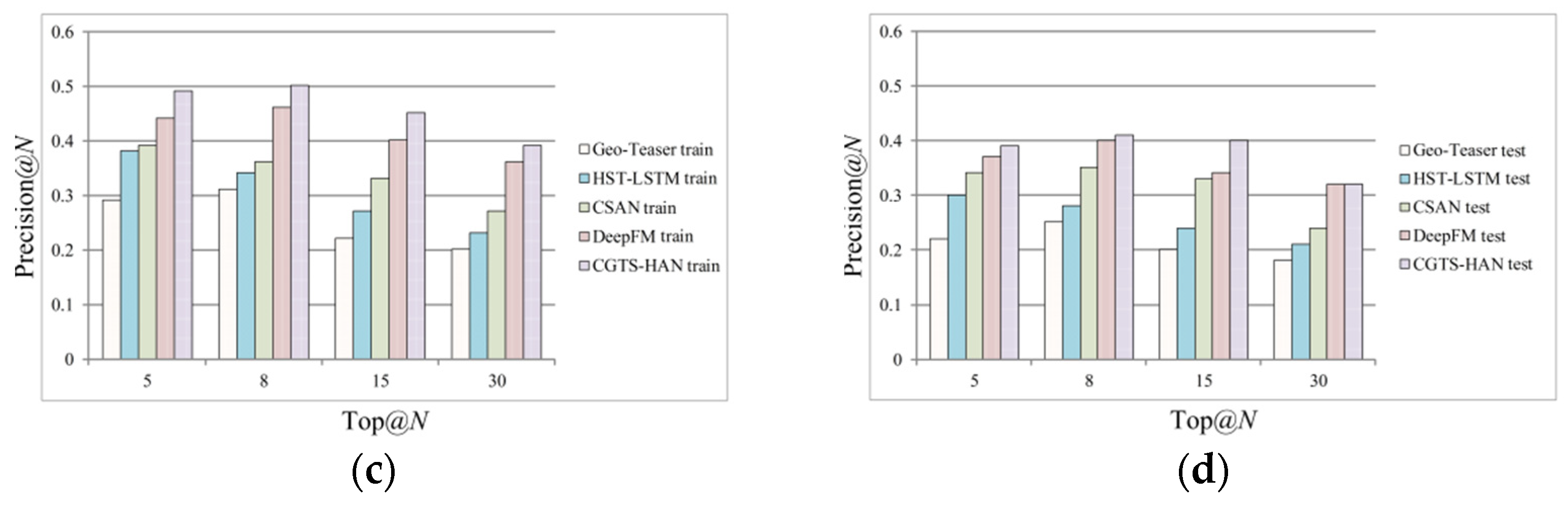
This paper conduct experiments with different values of the recommendation list size and extracts the experimental results of
N = {5,8,15,30} as samples. The experimental results of precision and recall are shown in
Figure 5 and
Figure 6.
It can be seen from
Figure 5 that, with the increase of
N, the Precision of the rest of the models except the HST-LSTM model increases first and then gradually decreases. Moreover, it can see from
Figure 6 that the Recall rate of all models increases with the increase of
N. To balance the effects of precision and recall, we select the top 15 POIs for recommendation in the experiment. In this case, the precision of the proposed CGTS-HAN model on the Foursquare and Yelp datasets is 18% and 6% higher than that of DeepFM, and the Recall is 10% and 6% higher, respectively. This verifies the good effect of CGTS-HAN integrating sequence, geographic, time and social influencing factors. Experiments demonstrate that adding auxiliary information of social connections helps improve POIs recommendation performance and, at the same time, confirms the effectiveness of modeling with attention networks.
5.4.3. Parameter Analysis
In this experiment, the parameter sensitivities of time influence weight coefficient α, geographical influence weight coefficient β and learning rate η were quantitatively analyzed by the control variable method. This part of the parameter analysis uses the preprocessed data set and does not divide the training set and the test set.
From
Figure 7, we can see how the parameters affect the precision and recall of CGTS-HAN. In order not to tune A, this paper integrates
η into α and
β in the tuning process (that is,
α ×
η →
α,
β ×
η →
β.) and then tunes the two parameters of
α and
β to weigh the influence of time and geographical factors. In order to ensure convergence, we make the values of
α and
β as small as possible in the experiment. At the beginning of the tuning, we assume that the values of
α and
η are equal and change the learning rate by tuning
α. The experimental results show that when α increases, the precision and recall rate of the experimental model maintain an upward trend as a whole, and the growth rate slows down as the coefficient value increases. When α is equal to 0.05, the precision and recall performance of the model in this paper is balanced and reaches the best. Therefore, we assume that α is equal to 0.05 and remains unchanged by tuning the
β value to observe the changes of
in the precision and recall rate of the model in the [0, 2] interval.
Figure 7 shows that the CGTS-HAN can achieve the best recommendation performance when
∈ [0.5, 1].
5.4.4. Time Complexity Analysis
Complexity. For one check-in trajectory, learning the temporal embedding model costs O(T·K·d), where T, K and d denote the context window size, the number of negative samples and the latent vector dimension, respectively. For the dynamic preference () learning in Algorithm 1, we sample m unvisited POIs, which can generate maximum O(m2). For each trajectory, the learning procedures cost O(m2·d). Therefore, the complexity of CGTS-HAN is O(m2·d·), where denote the user trajectory length.
Scalability. Generally, POIs are sparse in LBSN, and the number of check-in POIs is greater than the number of unchecked POIs. Furthermore, in order to make the model more efficient, we use Negative Sampling for optimization. The calculation time of each iteration of Equation (21) is approximately O((·K)||), where K is the number of negative samples, and || is the training set size. In fact, the values of and K both satisfy a relation (, K < <||). Therefore, as the check-in trajectories distribution of POIs in LBSNs follows PLF, the time complexity of CGTS-HAN proposed in this paper is linearly related to the number of check-in training sets ||, which also guarantees that CGTS-HAN to parallel the parameter updates and scalable on large datasets.
6. Conclusions and Future Directions
This work studies the use of contextual information and interest preferences of users’ location-based social networks to recommend the next POI for users in the IoT environment. This paper proposed a new next POI recommendation model named CGTS-HAN, which can learn the contextual features of users’ POI more accurately than other models. The model aims to recommend the next POI according to the user’s historical trajectory, integrates the user’s current geographical location and time and considers its social influence to model the user’s dynamic preferences. In particular, the model can infer users’ interest preferences based on their social information to provide high-quality recommendations in the IoT environment when users have little or no activity history. Experiments are conducted on two datasets based on geo-social information, and the results demonstrate the effectiveness and efficiency of the method.
At present, the CGTS-HAN model uses offline training data, and future work will consider developing effective online training data to improve the accuracy of recommendation results. At the same time, sophisticated distributed representation methods can be developed to improve the next POI recommendation task.


