1. Introduction
Various fields have been promoting Wireless Sensor Networks (WSNs) in recent years, including industrial, environmental, and natural hazard monitoring [
1,
2]. In particular, WSNs have been actively introduced for risk management and natural hazard monitoring and prevention, where more attention is required to develop innovative and autonomous solutions to counteract life-threatening natural disasters [
3,
4,
5]. In this regard, continuous field monitoring systems for early warning detection is highly needed to enable hazard assessments and risk management. Along with the use of WSNs, integrating the Internet of Things (IoT) concept ensures the remote monitoring of large areas in real-time [
6,
7,
8]. Several Early Warning Systems (EWSs) are being developed to maintain control of vulnerable regions and facilitate immediate intervention in natural disasters. In particular, EWSs integrate WSNs to collect sensor data information, i.e., soil moisture, water level, soil inclination, and temperature, which are indicators of environmental changes. Furthermore, WSNs enable flexible and remote data collection, and analysis from distributed sensors [
3,
9,
10]. In landslide applications, critical requirements, such as real-time and continuous measurements, should be considered for designing and implementing the wireless network. A landslide early warning system (LEWS) must ensure flexible and remote access to the monitored area. Furthermore, LEWS provides accurate and precise information allowing the real detection of the landslide. Moreover, the LEWS needs to distinguish between normal weather change (e.g., temperature change between day and night) and landslide triggers (e.g., inclination of soil, severe change in water drop level). Therefore, the LEWS should be weather dependent for the identification of weather influence on collected data.
2. Related Works
In [
11], the authors developed a landslide monitoring system based on WSNs. Their sensor nodes integrated a pore water pressure sensor and strain gauges to measure the water pressure and soil displacement, respectively. However, the developed system depends only on the change of the sensor data information, which could trigger a false alarm. In [
12], a WSN architecture for real-time ground displacement monitoring was developed. However, the system is based on small-range communication only with a range of about 10 m. It is also highly energy-consuming since it uses the GPRS module to communicate the location data. In [
13], the authors proposed a WSN-based system for detecting the location of miners and identifying possible roof falls. Their system utilizes smart data gathering mechanisms using spatial and temporal correlation to detect disasters and earthquakes in mining areas. However, the system’s energy data transmission cost and sustainability are still limited. Another typical solution is to monitor the rainfall levels using WSN and water level sensors since rainfall is a major trigger of slope movement [
14,
15,
16]. In these systems, slope movement prediction is deduced by correlating the water levels and slope inclination. Hence, the slope information is also critical because it is more prone to false measurements. This could not satisfy the requirements of an acceptable margin of error. The use of specific sensors enables the supervision of landslides’ triggering parameters. However, the results cannot characterize the current situation in real-time and with reduced installation and maintenance costs. An interesting alternative is to perform ranging measurements using the transmission signals of the installed node, which bypasses the cost related to implementing specific sensors [
17,
18,
19]. Moreover, different works in the literature investigated the influence of weather changes on signal transmission [
20,
21,
22]. In [
22], meteorological parameters (i.g., humidity, atmospheric pressure, and temperature) proved to have a major influence on LoRa data transmission. Their work ensures accurate data transmission; however, correction related to weather influence is required for long-distance communication. Furthermore, their proposed system is expensive in terms of system and communication costs. In other works, the main focus was to provide accurate data collection and communication for dynamic nodes [
23]. The mobility of nodes provides an overview of the dynamic of the installation environment; however, it remains unsuitable for landslide detection. The complete network is dynamic in these scenarios and has no static references. In another study, the authors provide an interesting dynamic environment and surveillance solution [
24]. However, in their work, only simulations are carried out without considering external influences such as weather changes.
To conclude, the available works in the literature on WSN-based landslide early warning and prediction focus mainly on sensor information, location information, and weather forecasting. Most of them use GPRS data to identify affected regions, which is highly expensive. Moreover, short-range communication is used to collect sensor information, which requires the installation of additional nodes to ensure the coverage of the monitored area. Furthermore, sensor-based systems are prone to error, which affects prediction accuracy. Considering these aspects, a LEWS is developed, where the distance between installed wireless nodes is observed and used to identify the landslide occurrence. This definition helps to build a proactive risk management system based on weather conditions. In this study, the main focus is the design and installation phase of the LEWS and the monitoring activity. Furthermore, we present a preliminary analysis of slow-moving (cm/s) surface slide through wireless technologies. The main contributions of this work are summarized in the following points:
Design of an accurate ranging system to identify the node’s stability in terms of distance variation;
Investigation of the weather impact on the distance measurement with a focus on the temperature influence;
Use of Support Vector Machine (SVM) to classify the origin of obtained distance variation as a way for early landslide warning.
The paper is organized as follows. The proposed WSN system for landslide early warning is detailed in
Section 3. In
Section 4, experimental evaluation based on laboratory and field tests is provided. The collected measurement data is evaluated regarding system resolution and sensitivity to changes. The investigation related to weather changes is given and discussed in
Section 5. Later, a case study of landslide early warning is provided in
Section 6, where details on the deployed SVM model are provided and studied. A summary of the main characteristics of the WSN-based system is provided in
Section 7.
Section 8 concludes the presented work and opens new perspectives for future research.
3. Developed WSN for Landslide Early Warning Based UWB
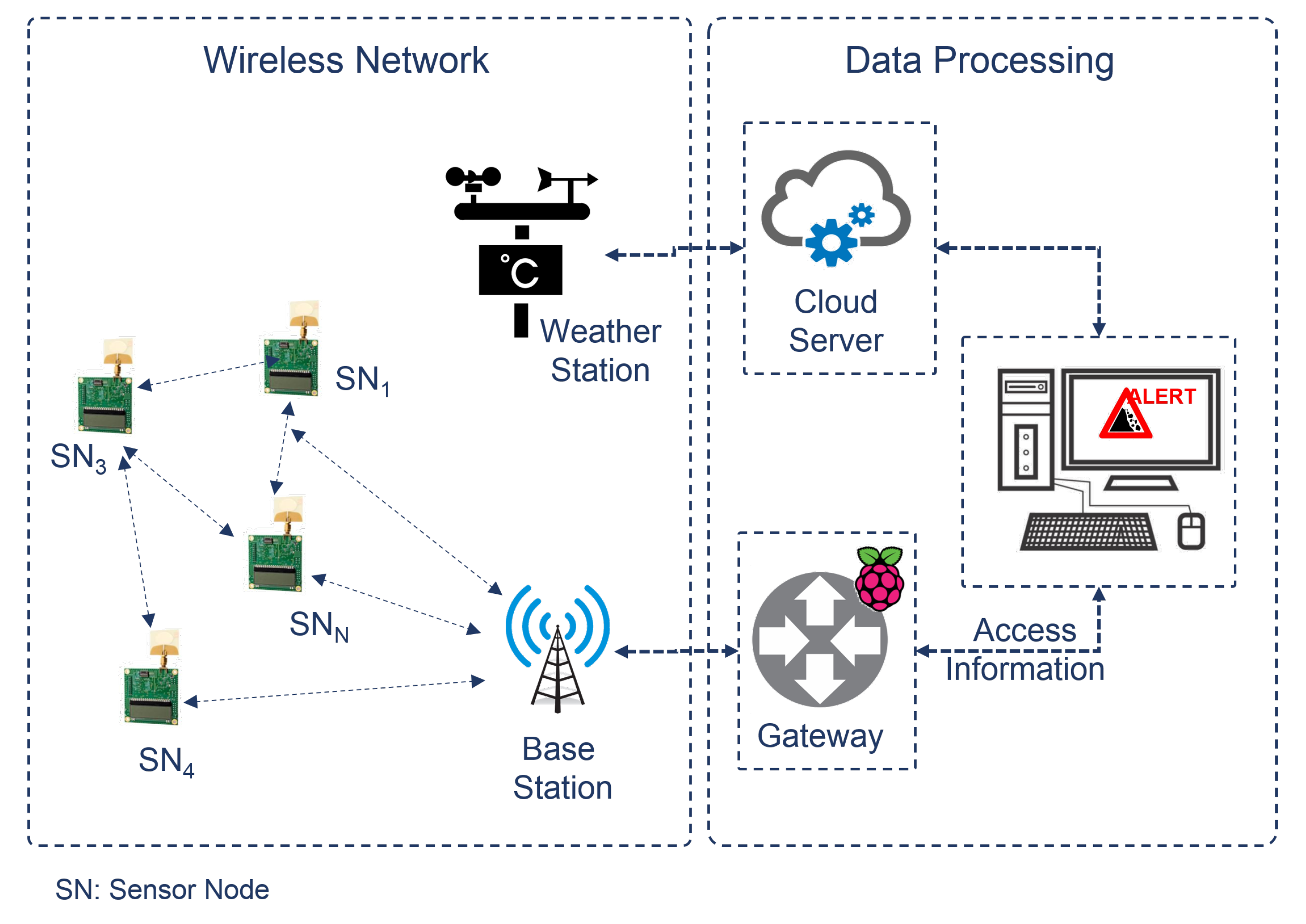
In this work, a landslide early warning system is developed using WSNs. It is based on the connectivity and ranging information between installed nodes in the field of interest. In particular, a ranging system is introduced to measure the distance between the deployed nodes and monitor the nodes’ current position and displacements. Distance information is collected via a raspberry gateway to ensure real-time and continuous data storage. The weather forecast is collected from a weather station connected to a cloud server where weather information is dynamically stored and foreseen. Later, the correlation between the weather parameters and distance variation is investigated at the processing unit (see
Figure 1).
The main novelty of the developed LEWS is to explore the ultra-wideband technology (UWB) to ensure accurate distance estimation between connected nodes. The investigation related to weather influence is introduced to ensure the stability and robustness of the LEWS. More emphasis on the UWB technology is highlighted in
Section 3.1. The distance measurement technique is presented in
Section 3.2.
3.1. UWB Technology for Distance Measurement
Ultra-wideband technology is a wireless communication protocol that uses electromagnetic radiation and wave propagation for communication and data transfer. It ensures high data rate transfer with high-ranging accuracy, low power consumption, and simple implementation. The UWB technology is known for its good performance, as it offers a good time-domain resolution allowing a precise location and tracking application with low power and low-cost on-chip implementation [
25]. In particular, Decawave (DW1000) sensor nodes are selected [
26], which use signals with a bandwidth of 500 MHz resulting in 0.16 ns-wide pulses. They have a fully integrated single chip, low-power, and low-cost transceiver following to IEEE 802.15.4-2011 standards. The main advantage of the selected UWB transceiver is its high data rate, as it can transmit pulses with a bandwidth of 500 to 900 MHz over a frequency of 3.5 GHz. This high temporal resolution allows for a theoretical accuracy of the ranging measurements approximated by
centimeters in LOS conditions as in [
27,
28]. Due to its high bandwidth and spectrum usage, the transmission power density of the UWB transceiver is limited to −41.3 dBm/MHz to avoid inter-system interference. The technical specification of the chosen Decawave ranging module is summarized in
Table 1. The accuracy and resolution of the UWB ranging are provided in
Section 4, with results from laboratory and test field experiments.
3.2. Two-Way Ranging Technique (TWR)
Two-Way Ranging technique (TWR) uses two delays related to signal transmission to determine the range between two communicating nodes. It determines the Time of Flight (
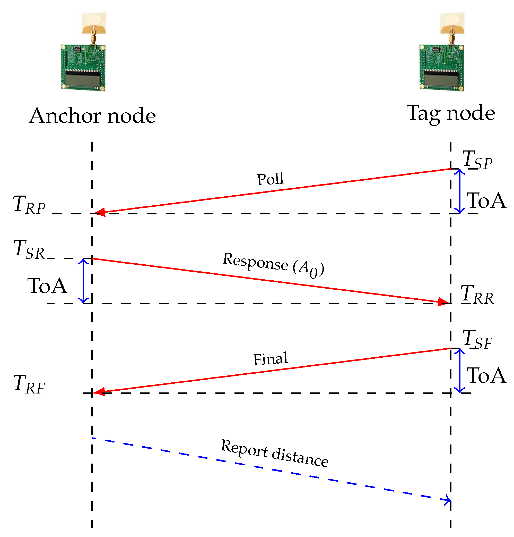
ToF) of the UWB RF signal and then calculates the distance between nodes by multiplying the time by the speed of light. In Decawave module, the TWR technique measures the distance between two nodes by exchanging three messages. The tag (this refers to the mobile node) initializes TWR measurements by sending a
message to the known address of the anchor (this refers to the fixed node) in a time frame referred to
(Time of Sending Poll). The anchor records the time of the
reception (
) and replies with the response message at time
. The tag records the time
when receiving the response message and composes a
message, where its address,
,
and
information are included. Based on the time reception of the final message
and the information provided in the final message, the anchor can determine the
ToF of UWB signal. The TWR implemented in Decawave is illustrated in
Figure 2, where two nodes are communicating. The
ToF is calculated using the timestamps of communicated signals as presented in Equation
1. Later, the distance between the tag and anchor nodes is calculated by multiplying the
ToF of the UWB signal by the speed of light
c as depicted in Equation (
2).
The distance between installed nodes is calculated and estimated based on the TWR. Later, the ranging system is explored in order to identify the effective time and space resolution of the Decawave system. The distance-ranging system is tested under different conditions. In the first part, it is evaluated in terms of stability and correctness. Then, the ranging system is observed with consideration of different weather changes. These evaluations help to build knowledge of the system’s resolution under normal and variable weather conditions.
4. Laboratory and Test Fields Investigations
This section describes the procedures adopted to validate the proposed system in a real environment. The prototype of the WSN system is designed and implemented to satisfy the requirements of high flexibility, rapid installation time, and limited investment costs. The test and evaluation of the WSN prototype include the following:
Laboratory tests: To prove the nominal performance of the prototype.
Early calibration tests and sensitivity analyses: To highlight the system’s dependency on environmental and physical parameters (e.g., temperature and humidity).
Landslide tests: The landslide tests are carried out with the use of a ready database.
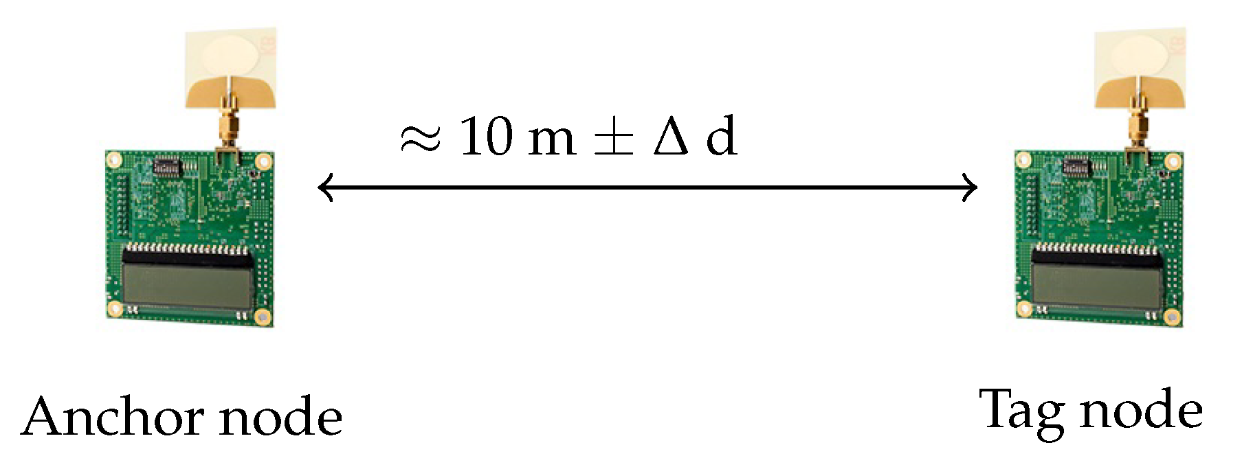
All measurements are realized under the LOS, enabling precise characterization of the system performance in free space and outdoor environments. Sampled results provide an experimental observation of the UWB-ranging system efficiency in an outdoor field. Two nodes are considered: one anchor and one tag node, where the anchor is fixed, and the tag node changes its position by translation with no change in the angular between both nodes. The distance in-between is varied manually to study the accuracy and stability of the ranging system, as depicted in
Figure 3.
The following quantifies the sensitivity and resolution of the ranging system. The measurement protocol is as follows: A new ranging session starts every 200 ms and runs for about 30 s. The data packet is composed of 32 bytes of Decawave information, which refers to the sensor data, for example, if existing, or the information about the location and signal quantity. The measurements were performed with the positioning of the nodes placed 15 cm above the ground to ensure the line of sight. In all our experiments discussed in this paper, we consider that the nodes are in LOS, i.e., without obstacles.
4.1. Experimental System Resolution Analysis
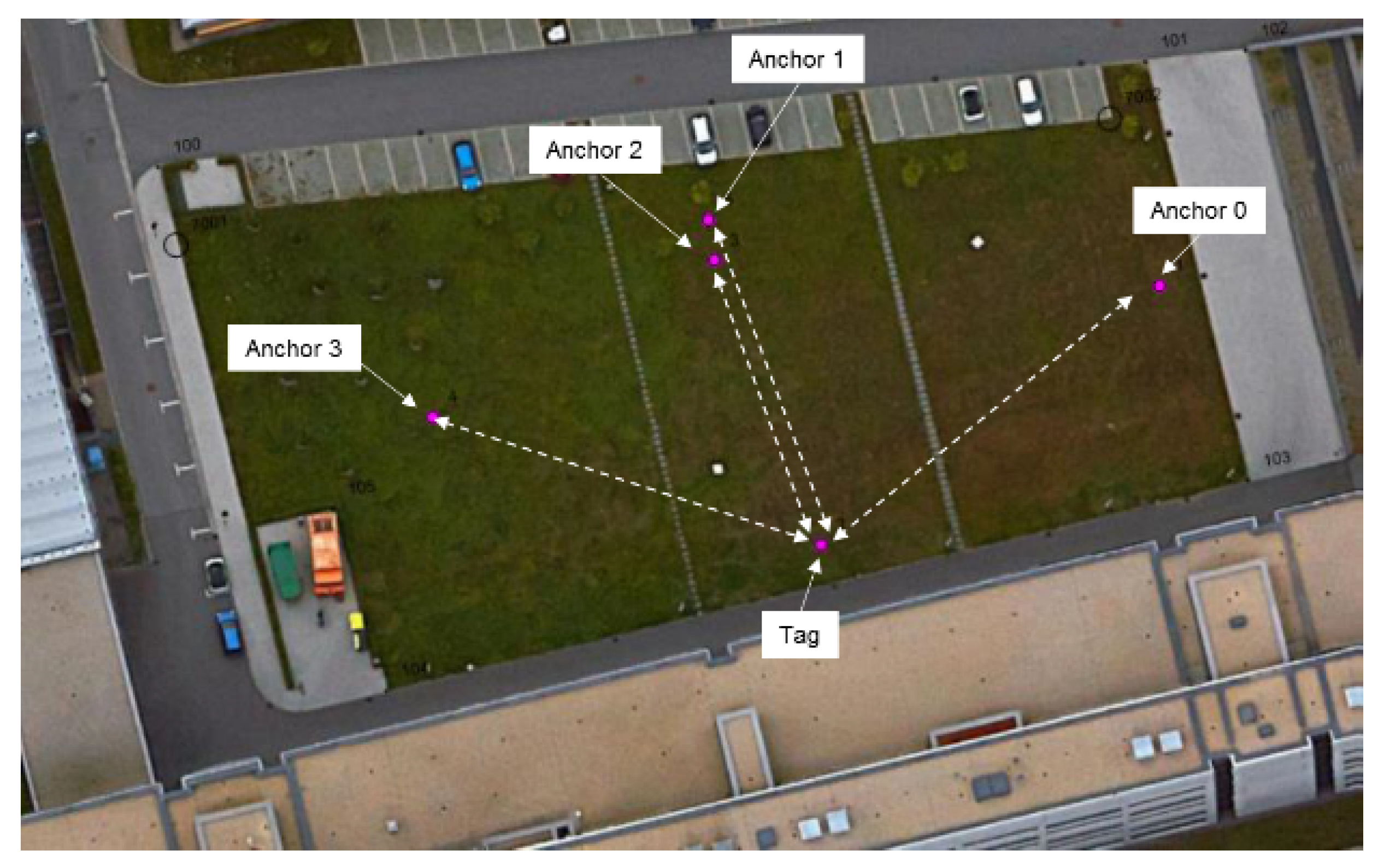
The ranging system is evaluated in terms of sensitivity and robustness for both large and small distance changes. In scenario 1 (see
Figure 4), one tag and three anchor nodes were installed in the network, and continuous measurement of the distance between them was achieved to identify the system stability over long experiments. Both nodes are fixed in the beginning, then a displacement is applied manually with increments of 5 to 10 m and a step size of 60 cm to 1 m for large and small variations, respectively. The obtained results are illustrated in
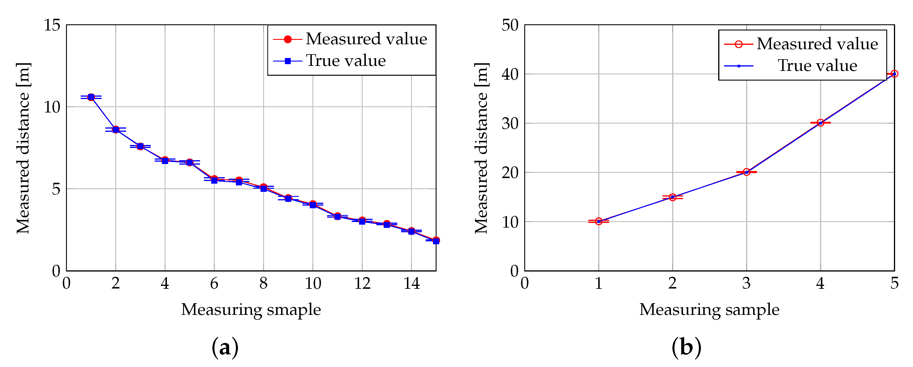
Figure 5.
In the first experiment (
Figure 5a), the two nodes are placed at a distance of 10 m in the beginning. Later, the tag node was moved over a
, which is in the range of [0.1 m, …, 2 m]. Each measurement trial was carried out over 50 min, and the distance was calculated from the Decawave anchor module. Collected results show that the system is able to act for both large and small distance variations. The estimated distance deviation is in the range of 3 to 13 cm for all stored samples. In the second experiment (
Figure 5b), the nodes were placed at a 10 m distance, and later the tag was moved with a step size of 5 m and 10 m. For a small distance variation, the average deviation is approximately 5.3 cm. For a large distance variation, the average deviation is approximately 8.8 cm. The accuracy is defined as how close the estimated distance obtained by the two-way ranging algorithm is to the known ground truth distance between the nodes. A good ranging accuracy should provide the match as closely as possible. With regard to this, the mean error of the collected data needs to be calculated based on Equation (
3).
where,
,
and
are the total number of samples, the estimated distance using the two-way range system and the real distance, respectively.
In
Table 2, samples of the obtained accuracy are presented, where the lowest achieved accuracy is estimated by 89.83% for 30 m, and the highest accuracy was noted at 10.6 m with 98.68%. The experimental accuracy is in the range of ≈94% for both small and large distances. This makes the Decawave ranging system reliable and accurate to be used for node displacement identification.
The Decawave module achieves a ranging resolution of 5 cm in LOS conditions. However, the accuracy of the UWB ranging measurements is also vulnerable to external factors, such as multi-path fading and receiver noise [
19]. The temperature variation is directly related to the crystal frequency stability of the Decawave, as the
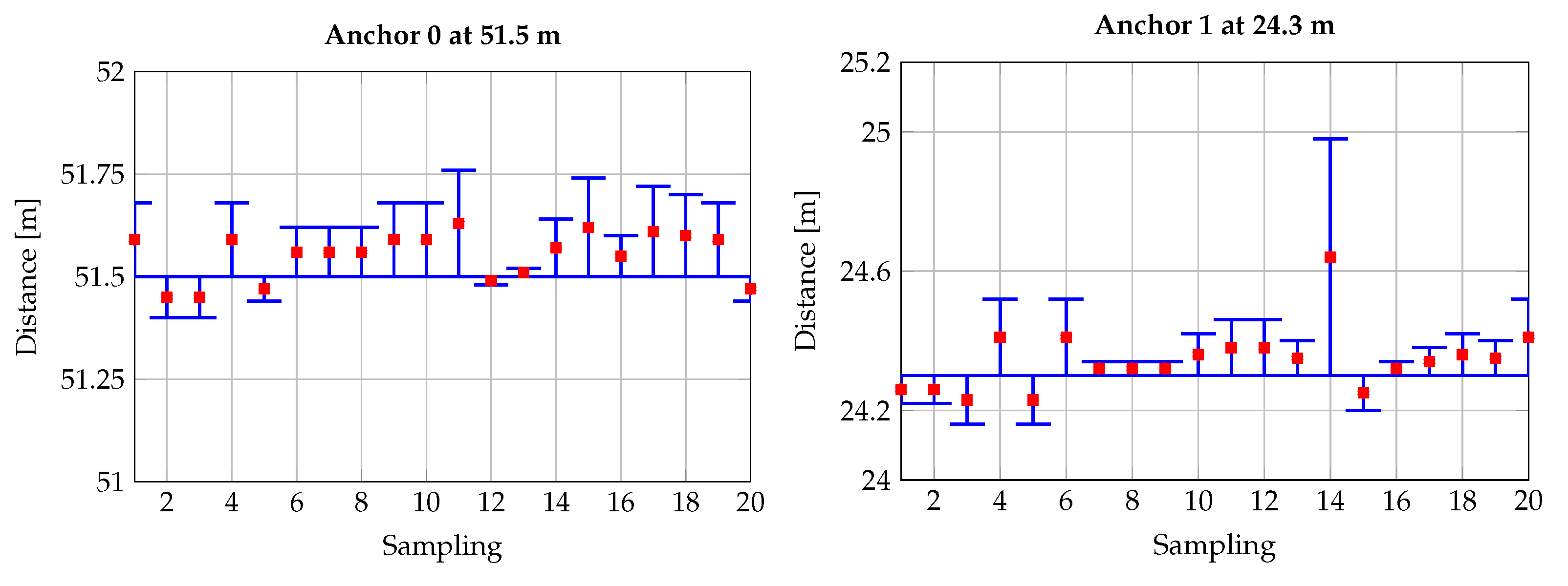
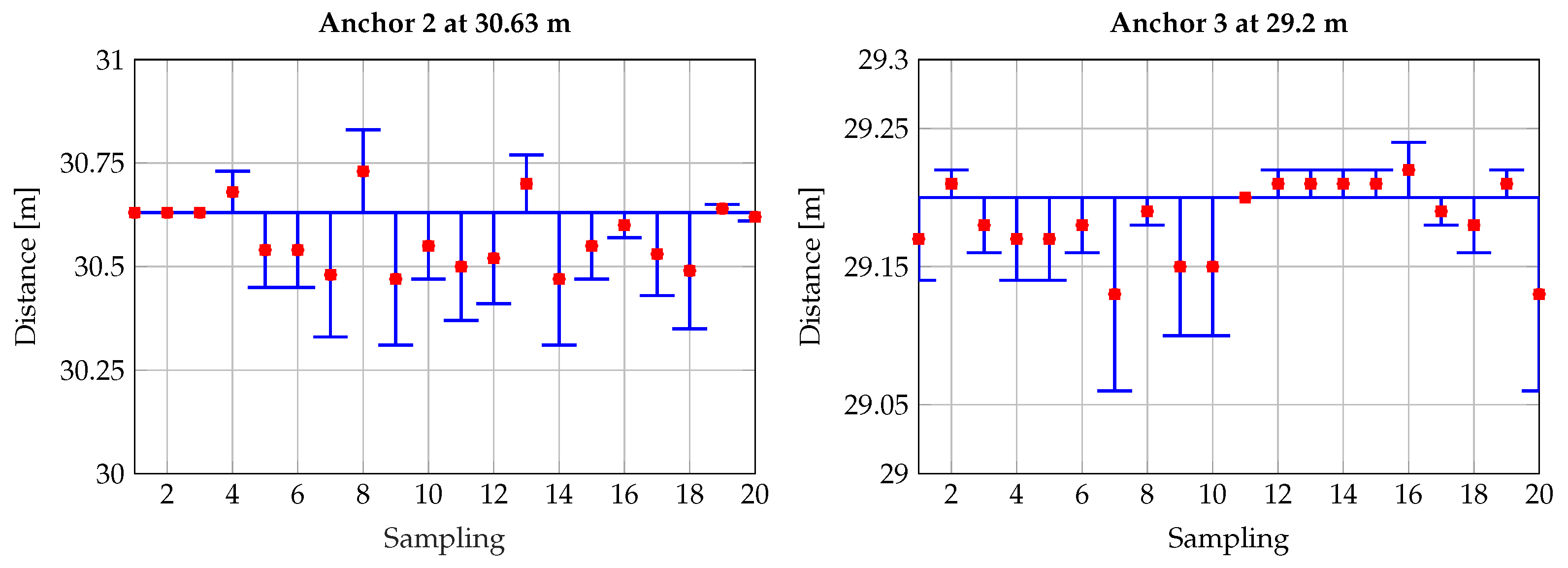
ToF is based on the speed of light and time synchronization. Thus, when subject to different weather variations, the system may have an additional deviation in the distance measurement. In the following, experimental characterization of the weather impact on the Decawave ranging system is provided. Experimental results show a deviation in the order of 5 cm. In fact, the average distance deviation is
,
,
, and
for
,
,
, and
, respectively (see
Figure 6). In practice, the nodes were not moved from their initial geographical positions. In this way, the distance deviation observed in the experimental data might result from external factors related to the deployment environment. For example, the presence of obstacles or objects in the deployment environment may cause shadows and interference with the signal, causing some noise in distance measurements. Additionally, changes in certain weather parameters could affect the electronic component of the ranging system, thus impacting both the system’s sensitivity and resolution, such as the humidity and temperature. Hence, the distance deviation can be triggered either due to signal interference or weather changes.
4.2. Energy Consumption Analysis
The energy consumption measurement of a wireless sensor node is carried out using the white box-based energy model, which considers the distance between the sender and the receiver and the number of sent bits. The energy of transmission and reception depends on the number of transmitted data bits over a distance
d. The energy consumption is calculated based on Equation (
4).
The current estimation of the wireless node is carried out using the four-wire energy measurement method. An efficient measurement instrument is used in this direction, Keysight Technologies E5270 8-channel Precision Measurement Mainframe [
29]. The instrument uses the four-wire method to estimate the consumed current for each state. The system relies on low resistance measurements by minimizing the influence of the electronic components’ resistance load on the measurements. In
Figure 7, the current consumption of the Decawave module is reported for each status. In
Figure 7a, the current consumption of the tag node is represented for each defined status, whereas in
Figure 7b the current profile of the anchor node is reported. The initialization of each node is similar and equal to 16.16 mA. During the ranging request, the tag node consumes around 142.17 mA to send the request to the anchor node. The anchor uses around 161.65 mA to receive the ranging request.
5. Analysis of the Influence of Weather Effects on Distance Estimation
5.1. Evaluation of Weather Influence on Distance Measurement
Distance ranging is performed to have an overview of the stability of the nodes in the network. Continuous measurements are required to build a stable and reliable monitoring system. In this direction, further experiments were realized to study the system’s sustainability for a long period [
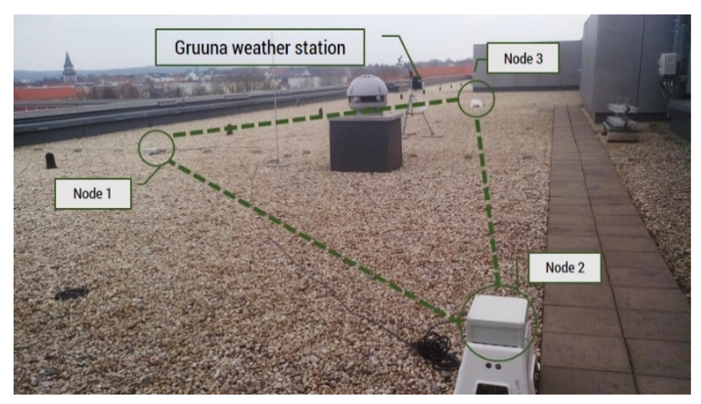
1]. In this work, different experimental tests were realized to explore the effect of weather changes on distance measurements. Three nodes were installed and maintained at fixed positions to examine the impact of weather changes on the Decawave ranging system. Two scenarios were realized to observe the distance variation between nodes at different weather conditions. In scenario 2 (see
Figure 8), the weather forecast system was placed between the installed nodes. In this case, the effects of the weather changes on the distance range are investigated.
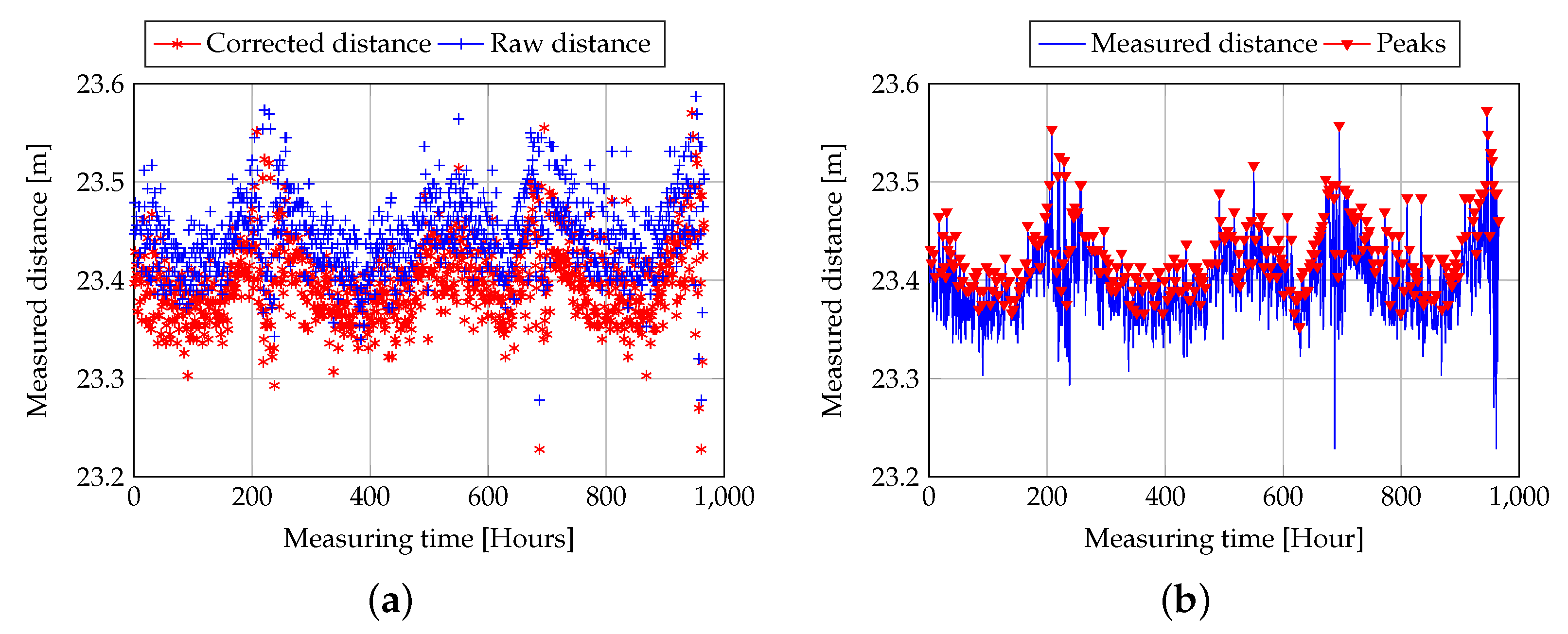
Further investigations related to the node’s environment are necessary to identify the source of the variation, such as weather changes or obstacles (Scenario 2). Only two Decawave nodes are installed in the field at a fixed distance of 23.4 m, illustrated as node 1 and node 3 in
Figure 8. Node 2 is used to collect the data, as a base station. Continuous distance ranging by Decawave is performed for two consecutive months. The obtained distance measurement data is filtered using a moving average filter to reduce the measurement variation related to systematic errors and the results are presented in
Figure 9a. These results show a variable deviation in the distance measurement with some sudden peaks. During this experiment, the field test environment has not been changed at any time; however, the obtained results are not stable, as illustrated in
Figure 9b.
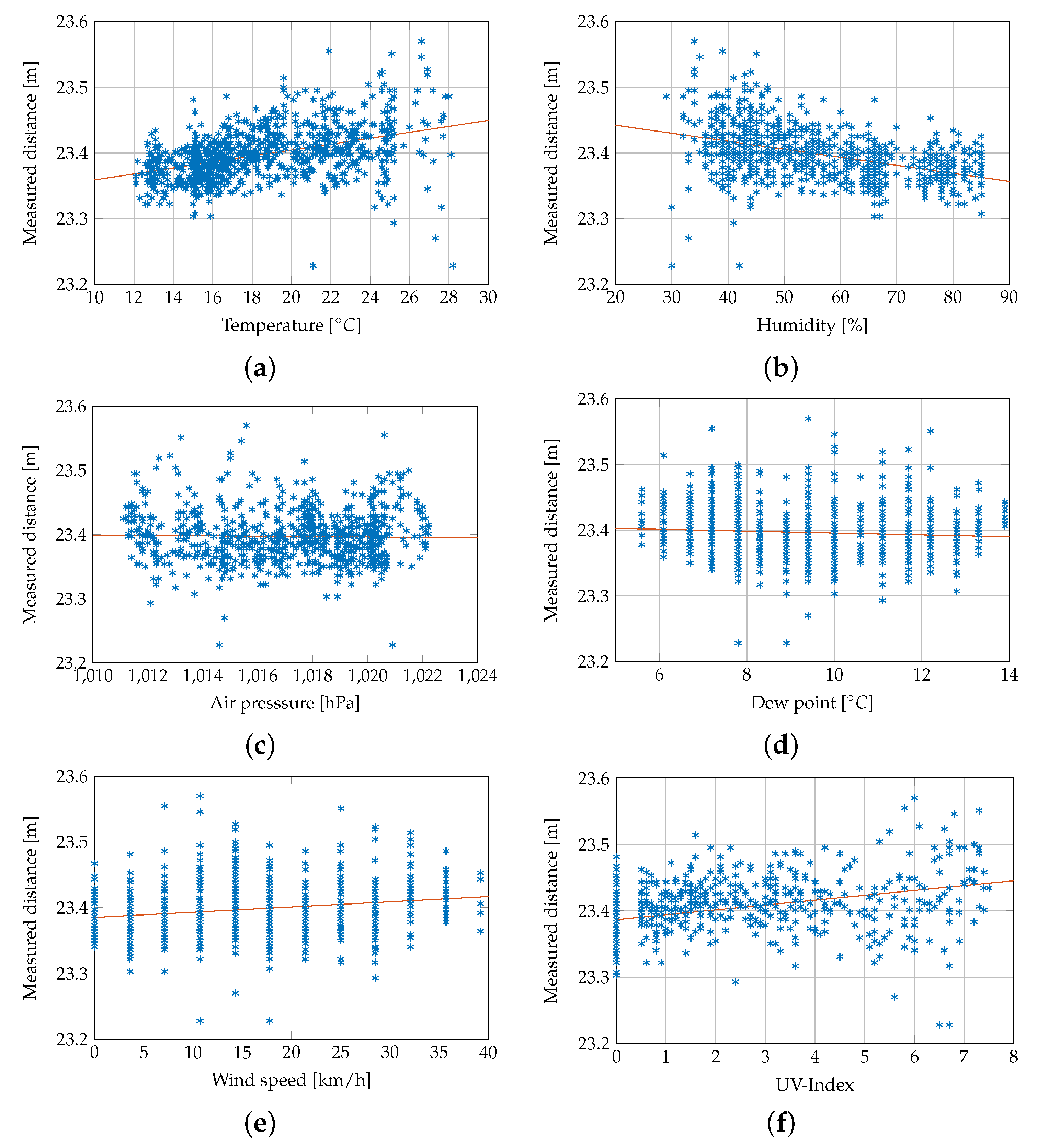
Weather values are associated with the measured distance between deployed nodes during these investigations. As seen in
Figure 10, each considered weather variation is plotted versus the distance, to identify the relationship between each weather parameter and the distance variation. The obtained results prove that the distance variation strongly depends on temperature, humidity, and solar radiation. Both the temperature and sun radiation present a strong positive correlation with the distance. The humidity is negatively correlated because the temperature and humidity are inversely proportional.
5.2. Weather Influence on Distance Correction
In order to define the dependency between weather parameters and distance variation, a correlation system is presented, where the mathematical correlation of two quantities
x and
y is considered [
29]. Considering the distance and temperature as two mathematical characteristics, the empirical correlation can be defined as in Equation (
5).
where,
n,
, and
are the number of samples and the average values of both quantities
x and
y, respectively.
In order to verify whether there is a linear dependence between
x and
y, a measure of their direct dependence of both characteristics is needed. Mathematically, it measures how closely the measuring points of two straight lines approach each other when placed in a coordinate system. A general correlation coefficient is formulated in Equation (
6).
By applying Equation (
6), the correlation between the temperature and distance and the solar radiation is estimated. The temperature presents a strong correlation equal to approximately 0.76, and the solar radiation presents a correlation of 0.6. The humidity is negatively correlated with the distance at 0.52. In the following, the temperature regression model is evaluated and tested.
A linear regression model based on the temperature variation is proposed to organize the obtained result, presented by Equation (
7), where
h is the regression hypothesis and
is the regression parameter to be estimated for the warning model (see
Figure 11).
The regression model shows that the retrieved data from the ranging system is closer to the proposed fitting system with a cost function defined as in Equation (
8).
Temperature correlation models can be used to correct distances between tags and anchor nodes, and the impact of temperature on actual distance variation can be eliminated. A comparison between the raw and the temperature-corrected data is illustrated in
Figure 11. A series of measurements are carried out to identify the impact of the regression model on the distance measurement correction. The obtained results are illustrated in
Table 3.
The summarized values in
Table 3 illustrate that the improvements are mainly in the standard deviation. They show an improvement with 33% and 29%, respectively, compared to the raw values. The fluctuation in the first quarter of the distance measurement series has a negative effect. The temperature values of the weather station can not explain this. It is remarkable, however, that this curve occurs reproducibly over several days at midday. Nodes are installed at the rooftop of the building. Once a day, sensor nodes are in the shadow of the antenna, while the weather station is exposed to full sunlight. This can explain this anomaly in the fitting temperature-distance response. To this end, experimental investigations on the distance-ranging system are realized. Various meteorological variables are associated with the distance ranging system to identify any correlation and dependency of the distance ranging deviation with the weather change. Results show that the distance measurement variation is strongly related to temperature and solar radiation changes.
6. Warning System for Landslide
During this study, we examine an early warning system for landslide detection. The proposed system consists of sensor nodes installed in a specific area and can communicate their ranging information through the WSN. The distances among installed nodes are continuously observed. In addition, a weather station is used to monitor the weather condition. Typically, the distance variation between stable nodes could be due either to systematic or random errors. In the first case, the distance variation is resultant of the ranging system capabilities, resolution, and calibration. In the second case, the distance variation can occur due to random and unpredictable effects, such as severe weather changes, node failure, obstacles, or movement. In this case, the obtained estimated distance may present various random deviations; however, estimated distance values still cluster around the true value. In this direction, it is essential to efficiently study the range system’s performance and define the normal working condition so that an early warning could be triggered in case of dramatic change.
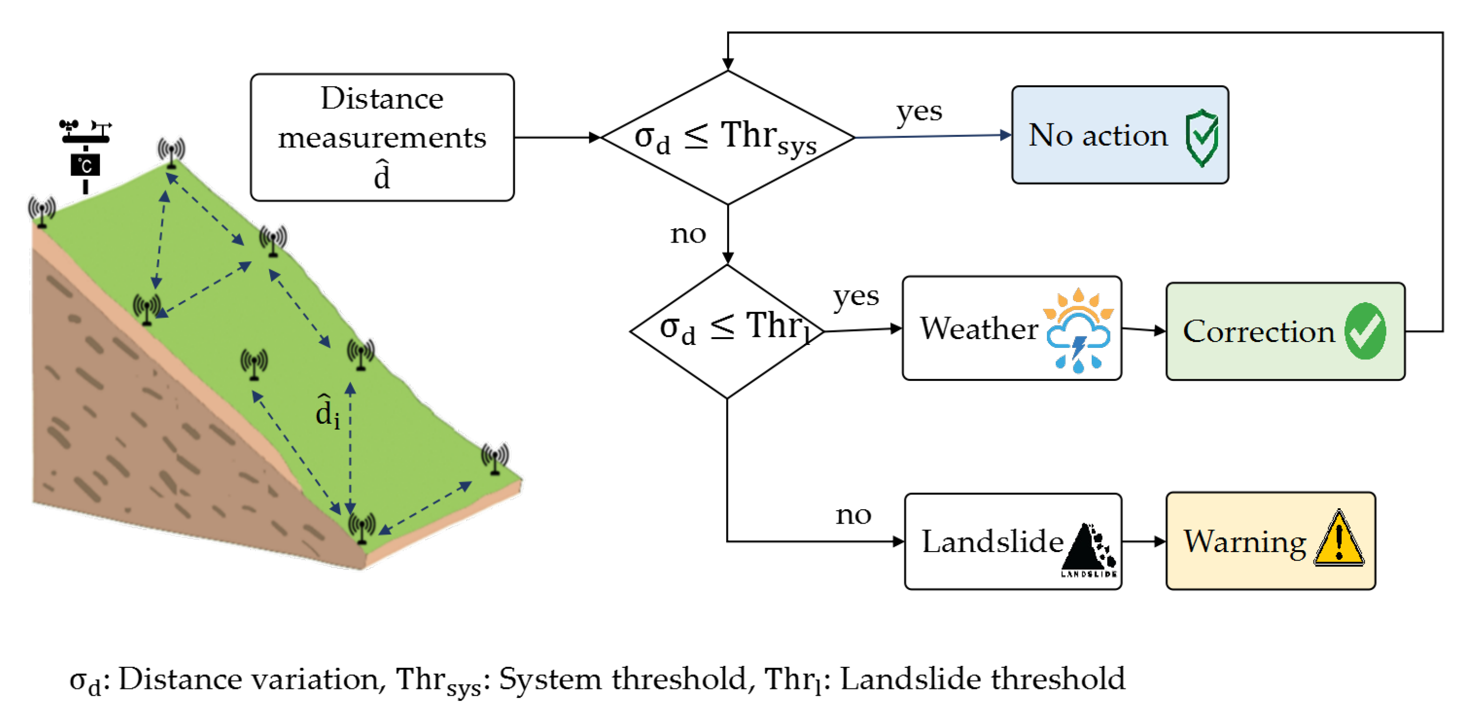
The proposed landslide warning system comprises two main blocks: Distance measurement and validation, data analysis, and classification. In the first block, distances between installed nodes are continuously estimated and compared to the real true values. Based on the obtained results and considering the respective weather information, the classification of the dataset is carried-out to generate a landslide warning alarm or not. Hence, special thresholds are needed to quantify the distance variation. In
Figure 12, an illustration of the proposed landslide early warning system is depicted. In the following,
and
are defined as the distance variation thresholds for the system and weather changes and for possible landslide occurrence, respectively. The determination of both thresholds should be performed carefully as it will serve later to identify possible landslide occurrence.
We estimate that the error obtained on the estimated distance measurements is related to the ranging system resolution and calibration, some weather changes, or actual node displacement. As a first step toward finding the cause of the error, it is essential to analyze and compare the measurement system’s performance in normal working conditions and during climatic changes. Accordingly, the variation is categorized into three categories: deviations caused by system malfunction, deviations caused by weather impacts, and deviations caused by node displacement, which results in landslide alarms.
6.1. Machine Learning Using SVM
The Machine Learning (ML) method provides an accurate and efficient solution to either predict or alert of a landslide occurrence. It provides an overview of the area of interest based on the collected data, which has a significant advantage over traditional data classification algorithms. Different techniques can be used as machine learning tools to classify and identify the collected data. The most common is the Support Vector Machine system (SVM) [
30], since it provides a simple and non-complex warning model. The SVM uses statistical data to create a classification model of the available information. It mainly implements two principles: The optimal classification hyperplane and the use of a kernel mathematical function. The hyperplanes serve to organize the collected samples into separate classes efficiently. As a definition, the distance between each hyperplane is called the classification margin, which represents the extreme border between classes. The kernel function helps transform the input samples into a dimensional space so they can be separated into classes [
31]. In practice, the classification hyperplane definition can be expressed as
, where
w,
b need to be determined for the classifier. Hereafter, the classification problem is solved by maximizing the margin distance between hyperplanes
. This problem can be solved by Lagrange multiplier method [
32]. For the case of only one constraint and only two choice variables, consider the optimization problem:
By applying a simple quadratic transformation on the optimization problem, the system is formulated as follows:
The proposed logic is that the variance of each weather parameter and distance deviation will be compared to the difference of every two consecutive values of distance and weather forecast and will only set logic 0 (landslide occur) when the difference of deviation value starts increasing from its variance, otherwise, in all other conditions the logic will remain 1, which means movement of the sensor is due to the weather changes or an NLOS condition. In the following, the main focus is attributed to the influence of temperature on distance measurement. The proposed logic is defined based on the temperature dependency model. The relative landslide indicator “
” is presented in Equation (
11). It considers the change in the temperature variation with the change in the distance range.
where
Diffdist is the difference of the distance values,
Distvar is the distance vector variance,
Difftemp is the difference of temperature values, and
Tempvar is the temperature vector variance.
Statistical data of the position estimation of installed nodes with the weather forecast are continuously collected and organized to build the classification model. Based on the distance variation margin the classifier is updated. Generally, the mean or average is the most common statistical tool used in various scientific experiments, but in our case, after analyzing the relation of climate with Decawave sensor deviations, variance analysis offers better results because the variance is more effective while sudden changes appear. In raw data, there is a pattern in the deviation values, which is varying continuously. As an assumption, the sensor node breaks down due to heavy wind, heavy rainfall, or because of the collision of wild inhabitants with the metal rod with which the node is connected. The distance increases immediately with a small difference. In this case, the comparison with the mean value starts showing a warning of a landslide, which is not the actual case.
6.2. Data Preparation and Measurement Procedure
The SVM model offers a more flexible method with a clear margin of separation between classes. Real movements have been excluded, and only the sensor nodes are moved manually if needed. In this work, the overall system contains three wireless sensor nodes, the tag node is continuously communicating with the anchor nodes, and their calculated distances are received at the control point simultaneously with climate forecasting parameters. At this point, the collecting system combines both data for pre-processing and makes timestamps for each measurement, then determines their variances and difference to design the logic of the SVM. The classification model description, as well as the system realization, are provided in the following sections. A detailed description of the SVM-based system offers insights into the working process of early landslide warning systems.
6.3. Results and Evaluation
6.3.1. Accuracy Assessment
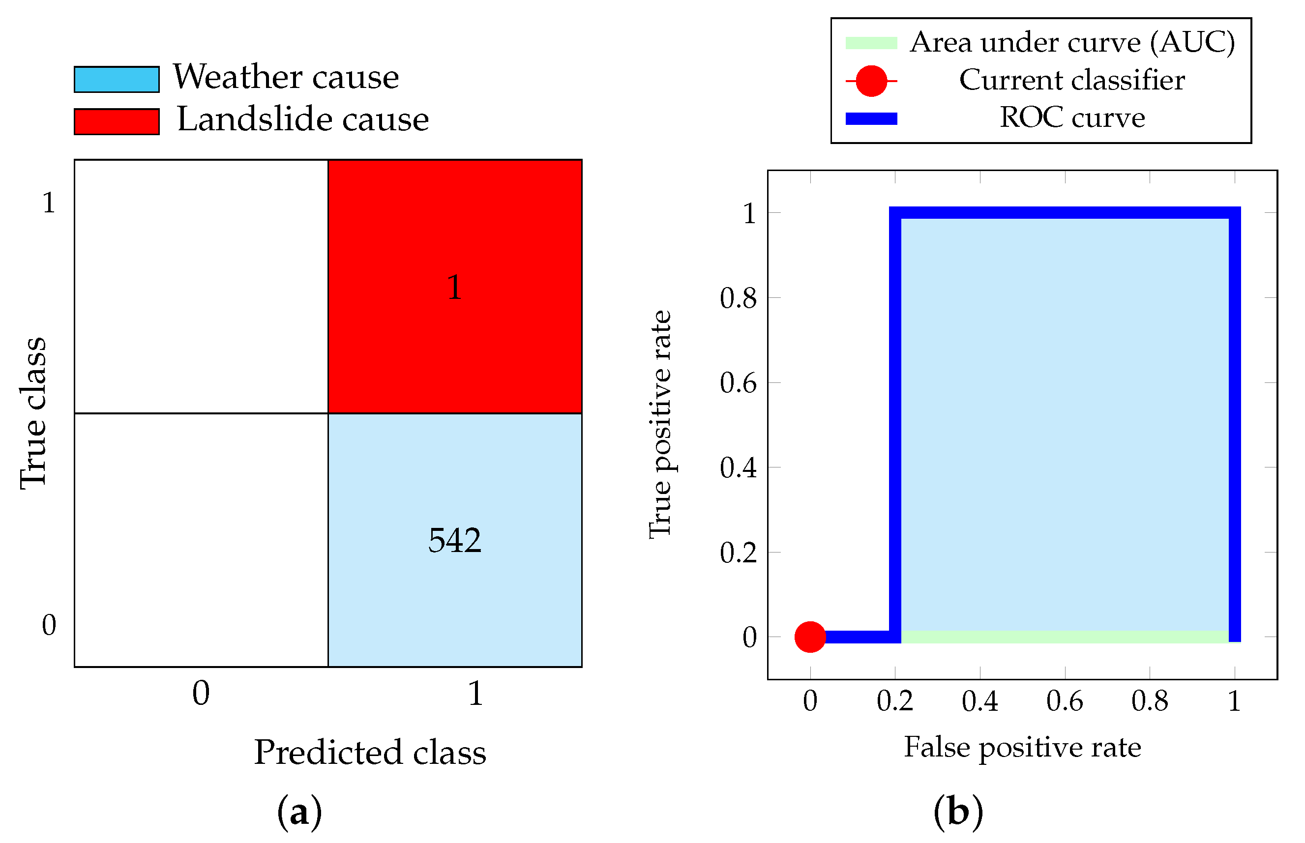
The accuracy assessment method used is the confusion matrix, which enables the evaluation of the results of the SVM method. In particular, the confusion matrix provides assessment methods for accuracy (AC), true positives (TP), false positives (FP), true negatives (TN), false negatives (FN), and precision (P). The accuracy AC is the overall performance of the warning method; in other words, how often does the algorithm correctly identify landslide and non-landslide warnings. The positive/negative portion of the labels refers to the identification of the warning: Positive for landslide warnings and negative for non-landslide warnings. The true/false nomenclature indicates whether the parameters correctly identified the evaluated area: true for correct identification and false for incorrect identification.
Figure 13 illustrates the confusion matrix of trained model warnings. In the given data set, out of 543 samples, only one data point belongs to the 0 class, but the classifier predicts it as a class 1 member because its input pattern is the same as class 1. Here, 0 means negative while 1 is represented as positive. The first box of the extreme left corner represents a true negative (TN) ratio, which means there is a landslide in the tested data and the model predicts it accurately. The first box of the second column shows that samples contain landslide data, but the model predicts it as no landslide, which is a false positive (FP). The first box of the second row shows that there is no landslide while the model predicts it as a landslide, which is a false negative (FN). The fourth and last box, which explains the ratio of the true positive (TP) shows that there is no landslide in the data set and the model predicts it accurately. There are two types of errors presented in the confusion matrix. Type 1 error is defined as FP and type 2 error is introduced as FN. The type 1 error is more dangerous because, in the FP condition, there is a landslide in the data set, but the model predicts it as no landslide and there will be no alarm warning. To determine the model accuracy, Equation (
12) can be derived from the confusion matrix:
The false positive type of error, which occurs in the results, can be negligible.
6.3.2. Receiver Operating Response
The Receiver Operating Characteristic (ROC) curve comprehensively assesses response sensitivity and specific features. When assessing landslide risk, the X-axis of the ROC curve shows the probability of the incorrect prediction of non-landslide points. Y-axis represents the prediction success rate of the disaster point, represented by the sensitivity. The accuracy of a prediction is expressed as the size of the area bounded by the curve and the abscissa. Accuracy increases as the curve moves closer to the upper left corner. The area under the curve (AUC) ranges from 0 to 1. The closer the AUC is to 1, the better the model is.
Figure 13 outlines the ROC model, in which the area under the curve shows the True positive class. The graph points out that as the model’s specificity increases, the model’s sensitivity also increases. In total, the warning model is achieved with an accuracy of 98%. The simulation time is 12.213 s, where the warning speed is approximately 3300 obs/s. To this end, a warning model based on corrected temperature distance data is provided. Further, implementations are required to include more weather parameters in the warning model. Indeed, the development and validation of a landslide early warning system are complex tasks that are never conclusively achieved on any single occasion but instead require robust and consistent support and investment over time for progressive improvements, periodic updates, and adaptations of the technology.
7. Discussion
The proposed LEW-WSN system can rapidly characterize a landslide early warning system in an emergency. Along with the portability and ease of deployment, the system can monitor the affected area and issue warnings. This section discusses the achieved results to examine the benefits and limitations of the LEW-WSN system and the UWB technology in general.
The main benefits of the LEW-WSN system for ground deformation monitoring are:
Easy and quick installation: The set up time of the system is very short. Only the anchors need to be placed in specific known locations in the stable area surrounding the unstable area, and the monitored anchor needs to be selected.
Flexibility: With LEW-WSN, different kinds of landslide, subsidence cases, or other ground deformation can be monitored without requiring specific adaptation.
Cost effective: LEW-WSN features low operating costs, making it possible to monitor a large area cost-effectively.
Accuracy: LEW-WSN’s integrated technologies provide the accuracy necessary to analyze different types of ground movements.
Scalability: It is possible to monitor movements in a network containing a large number of nodes.
8. Conclusions
In this paper, a landslide early warning system based on WSNs is designed, which take into account, the distance variation and weather changes. The TWR-based positioning algorithm for the UWB localization technique is used to measure the distance between nodes and have an overview of the nodes’ stability. After that, a weather forecast is gathered from an installed weather station. Measured distances and weather information are transmitted to the base station. A regression model is developed to identify the relation between the distance measurement variation and weather changes. A temperature correction is applied to the data. The developed polynomial model enables to predict the distance measurements and, increases the localization accuracy for temperautre correction. The proposed temperature correction method of distance measuremen enables reducing the standard deviation of the distance variation by 21%. In addition, the energy profile of the proposed system is reported for both the tag and anchor nodes. Later, a landslide early warning module is presented, where the weather impacts are identified and eliminated for an accurate landslide warning. A preliminary evaluation of the proposed early warning system is reported. In this evaluation, the system was tested by simulating some statistical data. Obtained results confirm that the proposed concept is suitable as an early warning system for landslide. Real measurement and validation of the prototype are initiated with an exploration of both the region- and site-specific parameters to improve the accuracy of the landslide system using wireless sensor networks.
Author Contributions
D.E.H. contributed by the experiment, measurement, manuscript concept, methodology, original draft writing, visualization, and editing. S.K., C.V., T.K. and O.K. contributed by writing of sections, reviewing, visualization, and editing. All authors have read and agreed to the published version of the manuscript.
Funding
The publication of this article was funded by Chemnitz University of Technology. This research was funded by the “Bundesministerium für Bildung und Forschung”, within the project “Verteiltes Sensornetz zur Böschungsüber wachung” (SENBÜ) (grantnumber 16ES0350K).
Institutional Review Board Statement
Not applicable.
Informed Consent Statement
Not applicable.
Data Availability Statement
Not applicable.
Conflicts of Interest
The authors declare no conflict of interest.
Abbreviations
The following abbreviations are used in this manuscript:
| EW | Early Warning |
| EWS | Early Warning System |
| GNSS | Global Navigation Satellite System |
| GPRS | General Packet Radio Service |
| GPS | Global Positioning System |
| GSM | Global System for Mobile communications |
| IoT | Internet of Things |
| LEW-WSN | Landslide Early Warning based on Wireless Sensor Network |
| LOS | Line of Sight |
| ML | Machine Learning |
| NLOS | Non-Line-of-Sight |
| SVM | Support Vector Machine |
| ROC | Receiver Operating Characteristic |
| TDMA | Time Division Multiple Access |
| ToF | Time of Flight |
| TWR | Two-Way Ranging |
| UWB | Ultra-wideband |
| WSN | Wireless Sensor Network |
References
- El Houssaini, D.; Guesmi, A.; Khriji, S.; Keutel, T.; Besbes, K.; Kanoun, O. Experimental investigation on weather changes influences on wireless localization system. In Proceedings of the 2019 IEEE International Symposium on Measurements & Networking (M&N), Catania, Italy, 8–10 July 2019; IEEE: New York, NY, USA, 2019; pp. 1–6. [Google Scholar]
- El Houssaini, D.; Khriji, S.; Besbes, K.; Kanoun, O. Wireless sensor networks in agricultural applications: Technology Components and System Design. In Energy Harvesting for Wireless Sensor Networks; Walter de Gruyter GmbH & Co KG: Berlin, Germany, 2018; pp. 323–341. [Google Scholar]
- Gamperl, M.; Singer, J.; Thuro, K. Internet of Things Geosensor Network for Cost-Effective Landslide Early Warning Systems. Sensors 2021, 21, 2609. [Google Scholar] [CrossRef]
- Reichenbach, P.; Rossi, M.; Malamud, B.D.; Mihir, M.; Guzzetti, F. A review of statistically-based landslide susceptibility models. Earth-Sci. Rev. 2018, 180, 60–91. [Google Scholar] [CrossRef]
- Cruden, D.M. A simple definition of a landslide. Bull. Eng. Geol. Environ. 1991, 43, 27–29. [Google Scholar] [CrossRef]
- Sinthuja, U.; Thavamani, S.; Makkar, S.; Gobinath, R.; Gayathiri, E. Chapter 22—IoT applications in landslide prediction and abatement—Trends, opportunities, and challenges. In Computers in Earth and Environmental Sciences; Pourghasemi, H.R., Ed.; Elsevier: Amsterdam, The Netherlands, 2022; pp. 319–325. [Google Scholar] [CrossRef]
- Butler, M.; Angelopoulos, M.; Mahy, D. Efficient IoT-enabled landslide monitoring. In Proceedings of the 2019 IEEE 5th World Forum on Internet of Things (WF-IoT), Limerick, Ireland, 15–18 April 2019; IEEE: New York, NY, USA, 2019; pp. 171–176. [Google Scholar]
- Kanoun, O.; Keutel, T.; Viehweger, C.; Zhao, X.; Bradai, S.; Naifar, S.; Trigona, C.; Kallel, B.; Chaour, I.; Bouattour, G.; et al. Next generation wireless energy aware sensors for internet of things: A review. In Proceedings of the 2018 15th International Multi-Conference on Systems, Signals & Devices (SSD), Yasmine Hammamet, Tunisia, 19–22 March 2018; IEEE: New York, NY, USA, 2018; pp. 1–6. [Google Scholar]
- Pecoraro, G.; Calvello, M.; Piciullo, L. Monitoring strategies for local landslide early warning systems. Landslides 2018, 16, 213–231. [Google Scholar] [CrossRef]
- Chae, B.G.; Park, H.J.; Catani, F.; Simoni, A.; Berti, M. Landslide prediction, monitoring and early warning: A concise review of state-of-the-art. Geosci. J. 2017, 21, 1033–1070. [Google Scholar]
- Fosalau, C.; Zet, C.; Petrisor, D. Implementation of a landslide monitoring system as a wireless sensor network. In Proceedings of the 2016 IEEE 7th Annual Ubiquitous Computing, Electronics & Mobile Communication Conference (UEMCON), New York, NY, USA, 20–22 October 2016; IEEE: New York, NY, USA, 2016; pp. 1–6. [Google Scholar]
- Salam, R.A.; Islamy, M.R.F.; Munir, M.M.; Yuliza, E.; Irsyam, M. Design and implementation of wireless sensor network on ground movement detection system. In Proceedings of the 2015 International Conference on Computer, Control, Informatics and its Applications (IC3INA), Bandung, Indonesia, 5–7 October 2015; IEEE: New York, NY, USA, 2015; pp. 89–92. [Google Scholar]
- Minhas, U.I.; Naqvi, I.H.; Qaisar, S.; Ali, K.; Shahid, S.; Aslam, M.A. A WSN for monitoring and event reporting in underground mine environments. IEEE Syst. J. 2017, 12, 485–496. [Google Scholar] [CrossRef]
- Piciullo, L.; Calvello, M.; Cepeda, J.M. Territorial early warning systems for rainfall-induced landslides. Earth-Sci. Rev. 2018, 179, 228–247. [Google Scholar] [CrossRef]
- Cuomo, S.; Di Perna, A.; Martinelli, M. Modelling the spatio-temporal evolution of a rainfall-induced retrogressive landslide in an unsaturated slope. Eng. Geol. 2021, 294, 106371. [Google Scholar] [CrossRef]
- Chinkulkijniwat, A.; Salee, R.; Horpibulsuk, S.; Arulrajah, A.; Hoy, M. Landslide rainfall threshold for landslide warning in Northern Thailand. Geomat. Nat. Hazards Risk 2022, 13, 2425–2441. [Google Scholar] [CrossRef]
- Mucchi, L.; Jayousi, S.; Martinelli, A.; Caputo, S.; Intrieri, E.; Gigli, G.; Gracchi, T.; Mugnai, F.; Favalli, M.; Fornaciai, A.; et al. A flexible wireless sensor network based on ultra-wide band technology for ground instability monitoring. Sensors 2018, 18, 2948. [Google Scholar] [CrossRef] [PubMed]
- Le Breton, M.; Baillet, L.; Larose, E.; Rey, E.; Benech, P.; Jongmans, D.; Guyoton, F.; Jaboyedoff, M. Passive radio-frequency identification ranging, a dense and weather-robust technique for landslide displacement monitoring. Eng. Geol. 2019, 250, 1–10. [Google Scholar] [CrossRef]
- Intrieri, E.; Gigli, G.; Gracchi, T.; Nocentini, M.; Lombardi, L.; Mugnai, F.; Frodella, W.; Bertolini, G.; Carnevale, E.; Favalli, M.; et al. Application of an ultra-wide band sensor-free wireless network for ground monitoring. Eng. Geol. 2018, 238, 1–14. [Google Scholar] [CrossRef]
- Ameloot, T.; Van Torre, P.; Rogier, H. Variable link performance due to weather effects in a long-range, low-power lora sensor network. Sensors 2021, 21, 3128. [Google Scholar] [CrossRef] [PubMed]
- Federici, J.F.; Ma, J.; Moeller, L. Weather impact on outdoor terahertz wireless links. In Proceedings of the Second Annual International Conference on Nanoscale Computing and Communication, Boston, MA, USA, 21–22 September 2015; pp. 1–6. [Google Scholar]
- Parri, L.; Parrino, S.; Peruzzi, G.; Pozzebon, A. Offshore lorawan networking: Transmission performances analysis under different environmental conditions. IEEE Trans. Instrum. Meas. 2020, 70, 1–10. [Google Scholar] [CrossRef]
- Gao, S.; Zhang, H.; Das, S.K. Efficient Data Collection in Wireless Sensor Networks with Path-Constrained Mobile Sinks. IEEE Trans. Mob. Comput. 2011, 10, 592–608. [Google Scholar] [CrossRef]
- Song, F.; Zhu, M.; Zhou, Y.; You, I.; Zhang, H. Smart Collaborative Tracking for Ubiquitous Power IoT in Edge-Cloud Interplay Domain. IEEE Internet Things J. 2020, 7, 6046–6055. [Google Scholar] [CrossRef]
- Digulescu, A.; Despina-Stoian, C.; Stănescu, D.; Popescu, F.; Enache, F.; Ioana, C.; Rădoi, E.; Rîncu, I.; Șerbănescu, A. New Approach of UAV Movement Detection and Characterization Using Advanced Signal Processing Methods Based on UWB Sensing. Sensors 2020, 20, 5904. [Google Scholar] [CrossRef] [PubMed]
- DecaWave. DW1000 User Manual; DecaWave: Dublin, Ireland, 2017. [Google Scholar]
- He, C.; Yuan, Y.; Tan, B. Constrained L1-Norm Minimization Method for Range-Based Source Localization under Mixed Sparse LOS/NLOS Environments. Sensors 2021, 21, 1321. [Google Scholar] [CrossRef] [PubMed]
- Uhlig, M.; Keutel, T.; Kanoun, O. Investigation of environmental influences on wireless localization techniques for outdoor applications. In Proceedings of the Sensor 2017 AMA Conference, Berlin, Germany, 30 May 2017; pp. 382–383. [Google Scholar] [CrossRef]
- Burmester, L.E.H. Lehrbuch der Kinematik: Für studirende der Maschinen-Technik, Mathematik und Physik Geometrisch Dargestellt. Die Ebene Bewegung. Mit einem Atlas von 57 lithographirten Tafeln. Atlas; A. Felix: Paris, France, 1888; Volume 1. [Google Scholar]
- Marjanović, M.; Kovačević, M.; Bajat, B.; Voženílek, V. Landslide susceptibility assessment using SVM machine learning algorithm. Eng. Geol. 2011, 123, 225–234. [Google Scholar] [CrossRef]
- Vapnik, V.; Mukherjee, S. Support vector method for multivariate density estimation. In Proceedings of the First 12 Conferences, Advances in Neural Information Processing Systems, Denver, CO, USA, 29 November–4 December 1999; MIT Press: Cambridge, MA, USA, 2000; pp. 659–665. [Google Scholar]
- Bertsekas, D.P. Constrained Optimization and Lagrange Multiplier Methods; Academic Press: New York, NY, USA, 2014. [Google Scholar]
Figure 1.
General architecture for the proposed wireless network for landslide early warning.
Figure 1.
General architecture for the proposed wireless network for landslide early warning.
Figure 2.
Average distance measurement based on the TWR technique for Decawave nodes.
Figure 2.
Average distance measurement based on the TWR technique for Decawave nodes.
Figure 3.
Schematic presentation of the experimental setup using the Decawave ranging system.
Figure 3.
Schematic presentation of the experimental setup using the Decawave ranging system.
Figure 4.
Decawave nodes at the inner courtyard of the university (Scenario 1).
Figure 4.
Decawave nodes at the inner courtyard of the university (Scenario 1).
Figure 5.
Experimental investigation on the Decawave measuring stability, representation of measurement series over a fixed distance: (a) small distance variation and (b) large distance variation.
Figure 5.
Experimental investigation on the Decawave measuring stability, representation of measurement series over a fixed distance: (a) small distance variation and (b) large distance variation.
Figure 6.
Experimental distance measurement in scenario 1 with one tag node and four anchor nodes , , , and . (red point: meaured distance, blue line: distance deviation).
Figure 6.
Experimental distance measurement in scenario 1 with one tag node and four anchor nodes , , , and . (red point: meaured distance, blue line: distance deviation).
Figure 7.
Current consumption over node’s status change in case of (a) tag and (b) anchor.
Figure 7.
Current consumption over node’s status change in case of (a) tag and (b) anchor.
Figure 8.
Investigation of weather influence in real-world (Scenario 2).
Figure 8.
Investigation of weather influence in real-world (Scenario 2).
Figure 9.
Experimental distance measurement between two stable nodes at a distance of 23.4 m: (a) corrected distance measurement considering average variation and (b) measurement peaks.
Figure 9.
Experimental distance measurement between two stable nodes at a distance of 23.4 m: (a) corrected distance measurement considering average variation and (b) measurement peaks.
Figure 10.
Presentation of measured distance variation with consideration of different weather parameters: (a) temperature, (b) humidity, (c) air pressure, (d) dew point, (e) wind speed, and (f) UV-Index.
Figure 10.
Presentation of measured distance variation with consideration of different weather parameters: (a) temperature, (b) humidity, (c) air pressure, (d) dew point, (e) wind speed, and (f) UV-Index.
Figure 11.
Raw and temperature-corrected measured values in comparison.
Figure 11.
Raw and temperature-corrected measured values in comparison.
Figure 12.
Schematic representation of the landslide early warning system.
Figure 12.
Schematic representation of the landslide early warning system.
Figure 13.
Investigation on the Receiver Operating Characteristic (ROC): (a) confusion matrix of the classifier and (b) evaluation of the system performance.
Figure 13.
Investigation on the Receiver Operating Characteristic (ROC): (a) confusion matrix of the classifier and (b) evaluation of the system performance.
Table 1.
Technical specifications of Decawave ranging system.
Table 1.
Technical specifications of Decawave ranging system.
| Parameters | Values |
|---|
| Communication standard | IEEE 802.15.4-2011 UWB compliant |
| Working frequency | 3.5 GHz |
| Supply voltage | 2.8 to 3.6 V |
| Communication range | Up to 75 m at 0 dBm |
| Power consumption | 154 mA ,
111 mA |
| Average distance deviation | 10 cm to 1 m |
Table 2.
Decawave measurement accuracy under LoS.
Table 2.
Decawave measurement accuracy under LoS.
| | Small Variation | Large Variation |
|---|
| | (60 cm 2 m) | ( = 5, 10 m) |
|---|
| Fixed distance in m | 10.6 | 8.6 | 3.3 | 3 | 1.8 | 10 | 15 | 20 | 30 | 40 |
| Measured accuracy in % | 98.20 | 98.86 | 96.90 | 92.48 | 93.84 | 92.13 | 94.68 | 90.05 | 89.83 | 94.35 |
Table 3.
Properties of the measured value series before and after deviation correction.
Table 3.
Properties of the measured value series before and after deviation correction.
| Sample | Correction | Minimum Value
in m | Maximum Value
in m | Mean Value
in m | Standard Deviation
in cm |
|---|
| 1 | without | 23.35 | 23.46 | 23.39 | 2.4 |
| 1 | with | 23.32 | 23.43 | 23.39 | 1.6 |
| 2 | without | 23.36 | 23.44 | 23.39 | 2.11 |
| 2 | with | 23.33 | 23.43 | 23.39 | 1.5 |
| Publisher’s Note: MDPI stays neutral with regard to jurisdictional claims in published maps and institutional affiliations. |
© 2022 by the authors. Licensee MDPI, Basel, Switzerland. This article is an open access article distributed under the terms and conditions of the Creative Commons Attribution (CC BY) license (https://creativecommons.org/licenses/by/4.0/).


