

An Incremental Learning Framework for Photovoltaic Production and Load Forecasting in Energy Microgrids

 ,
, 
 ,
,  ,
,
Abstract
1. Introduction
2. Related Work
2.1. RES Forecasting
2.2. Building Consumption Forecasting
2.3. The Need for an Incremental Learning Approach
3. Methodological Approach
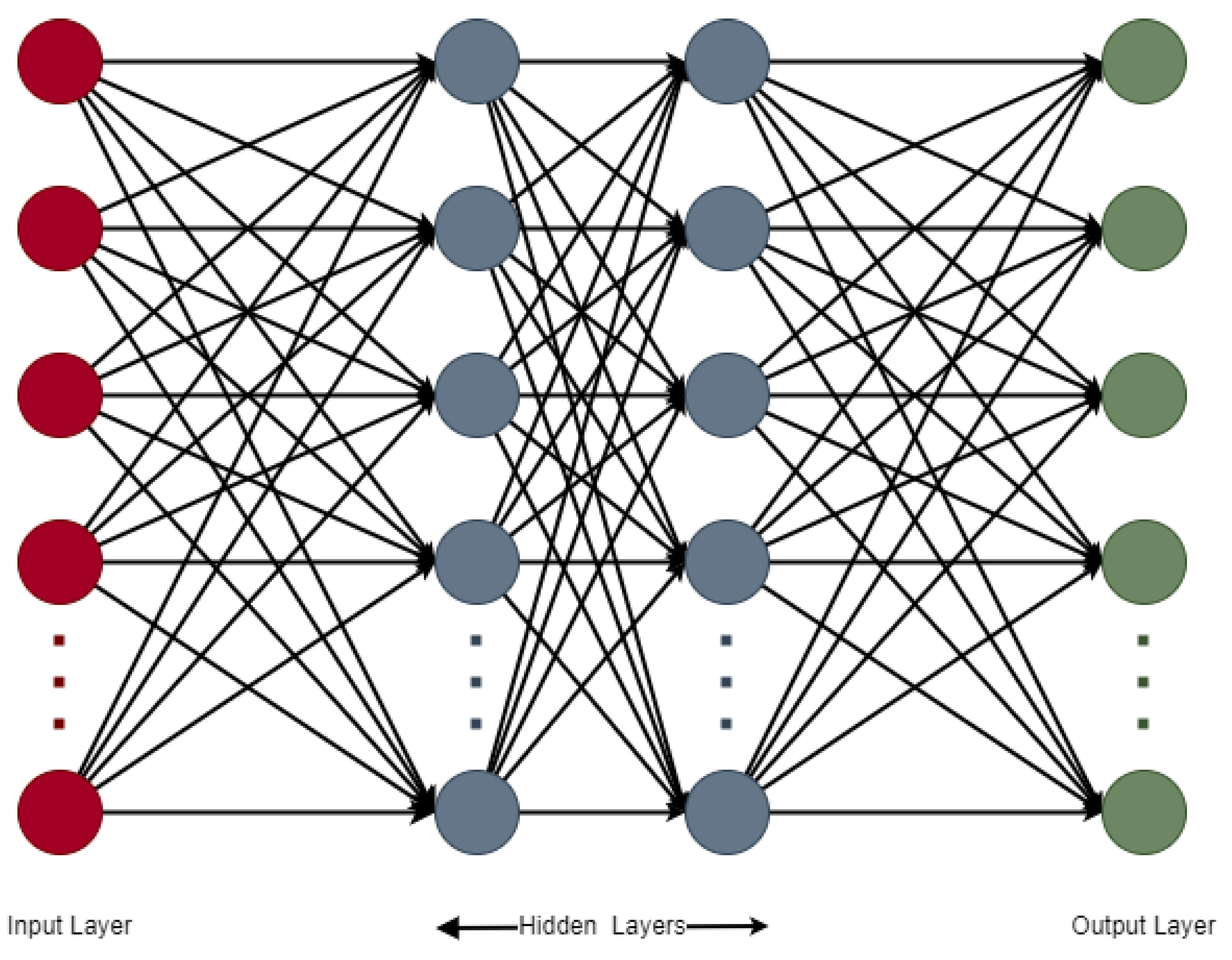
3.1. Multi-Layer Perceptron
3.2. Incremental Learning
3.3. Proposed Framework
4. Use Case
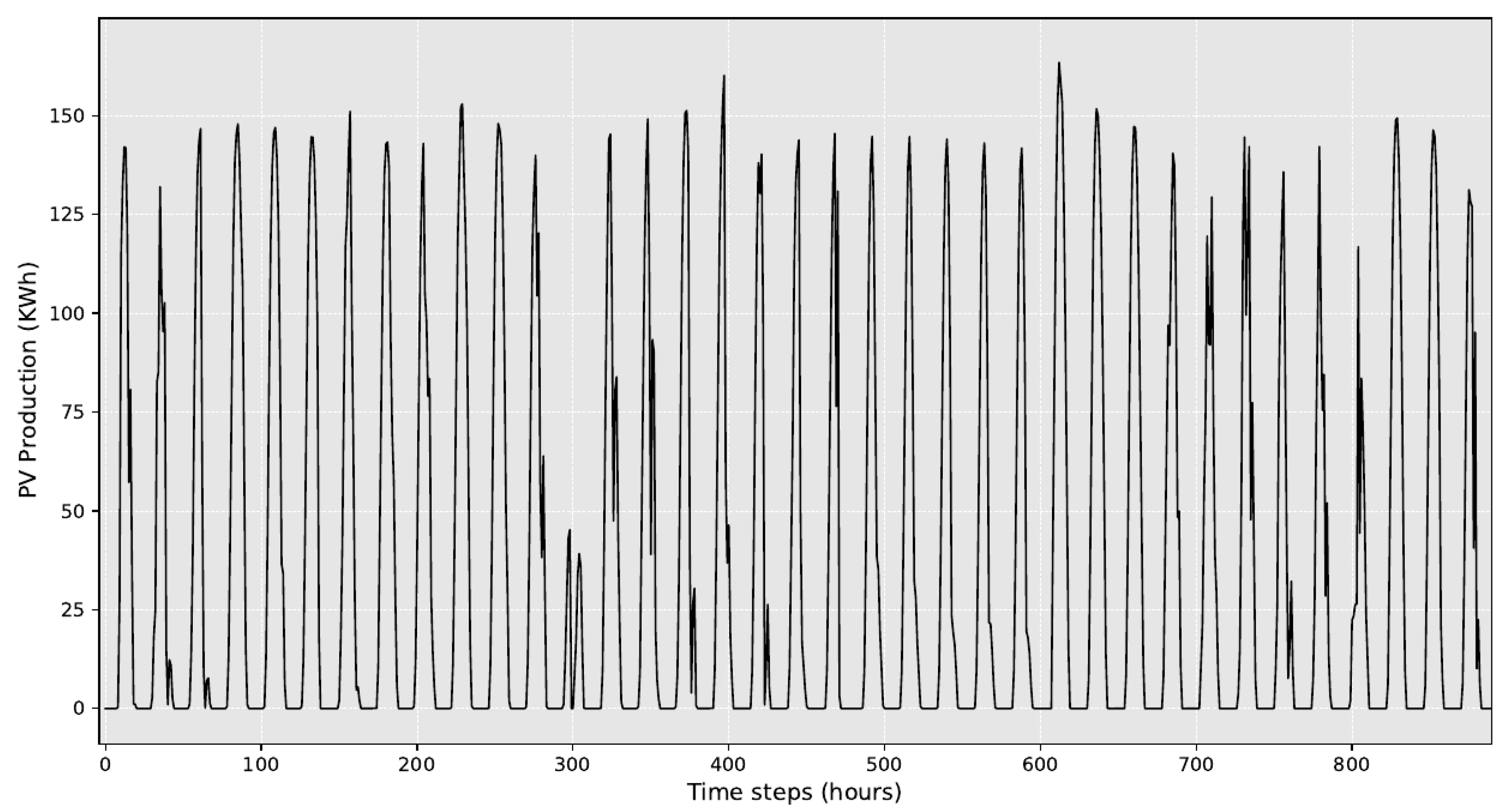
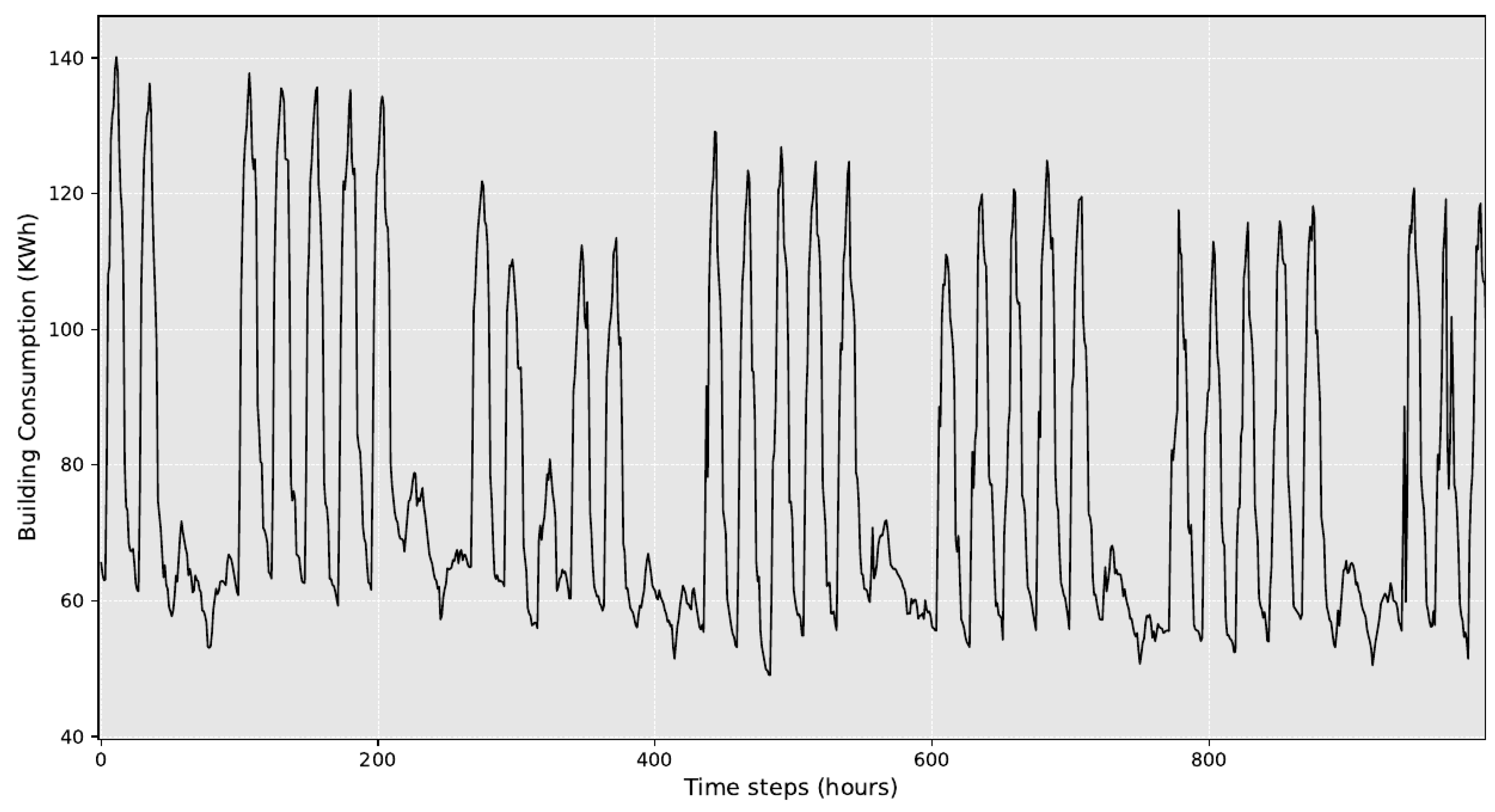
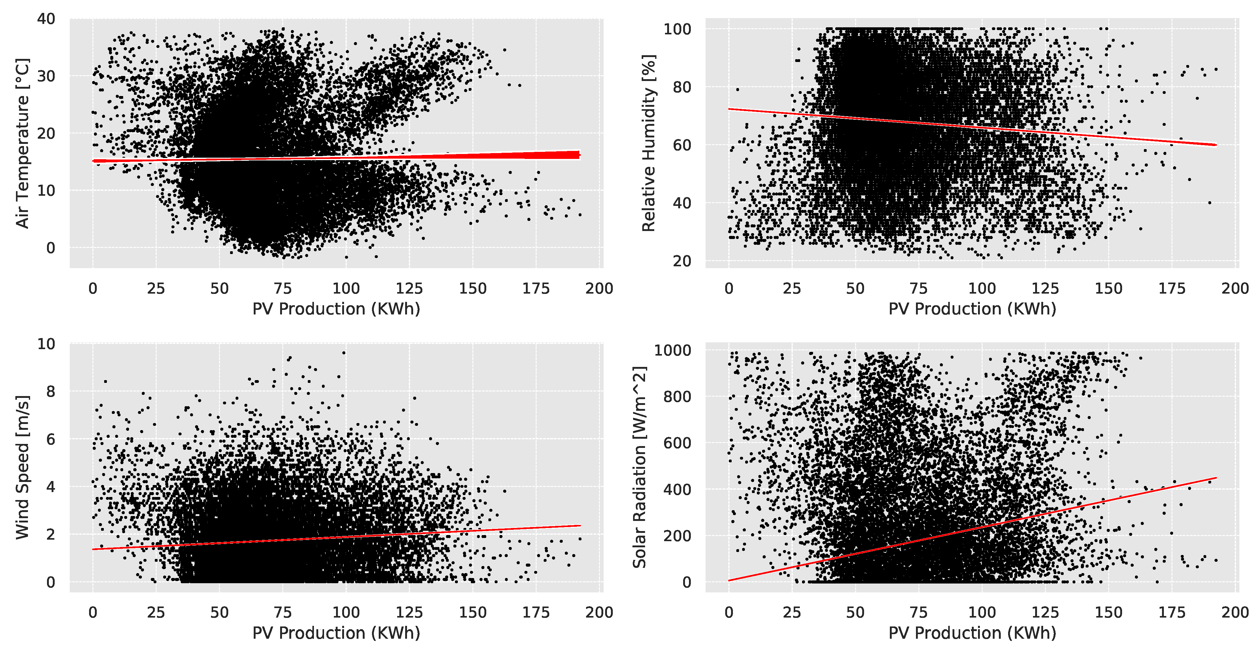
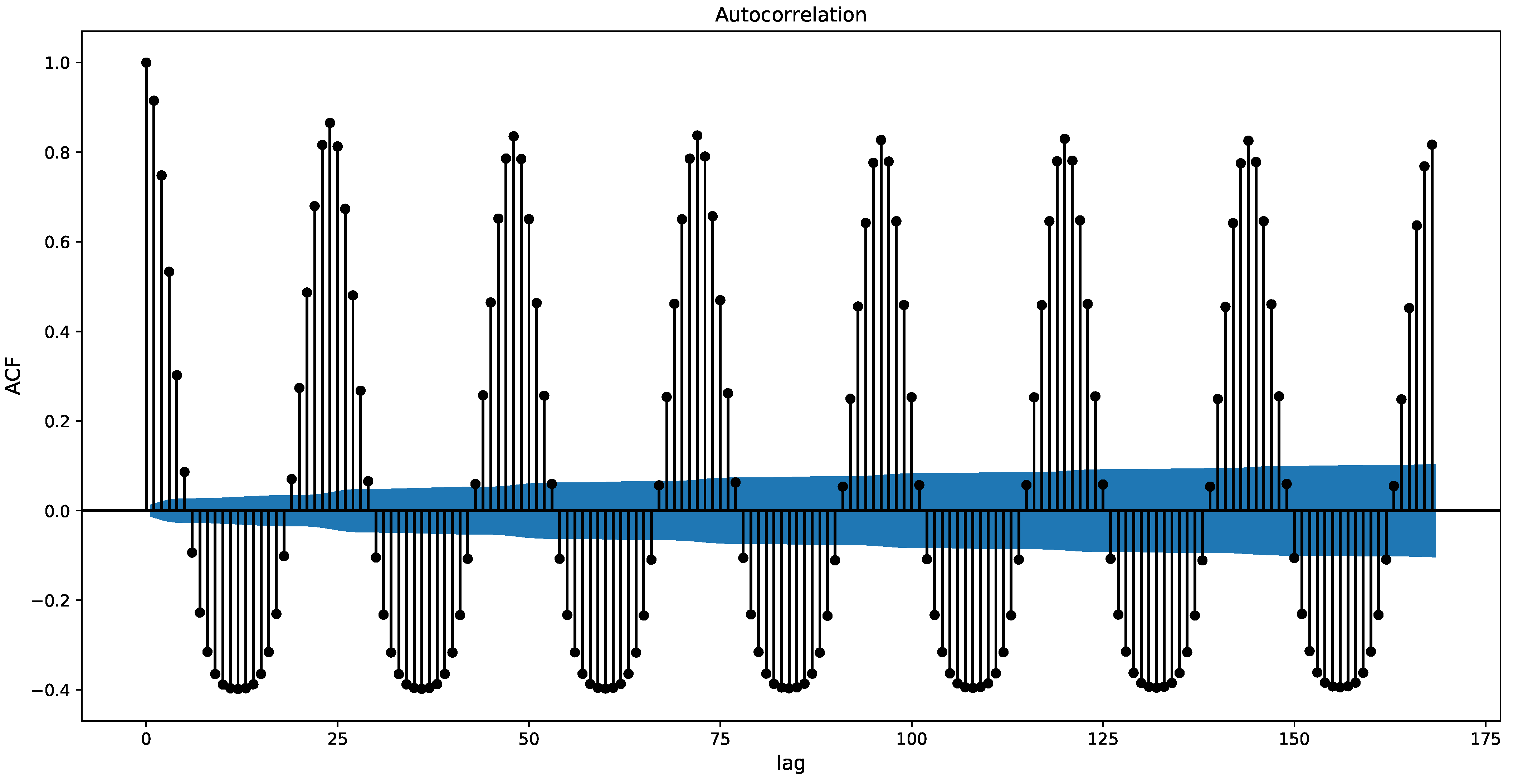
4.1. Datasets
4.2. Evaluation Metrics
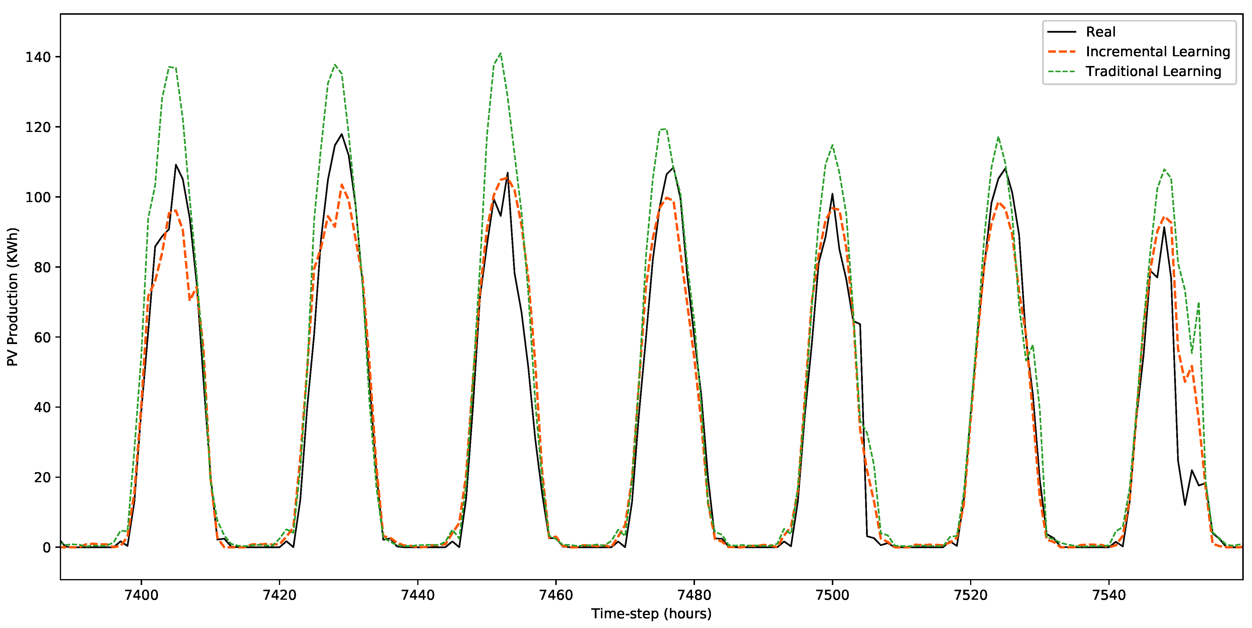
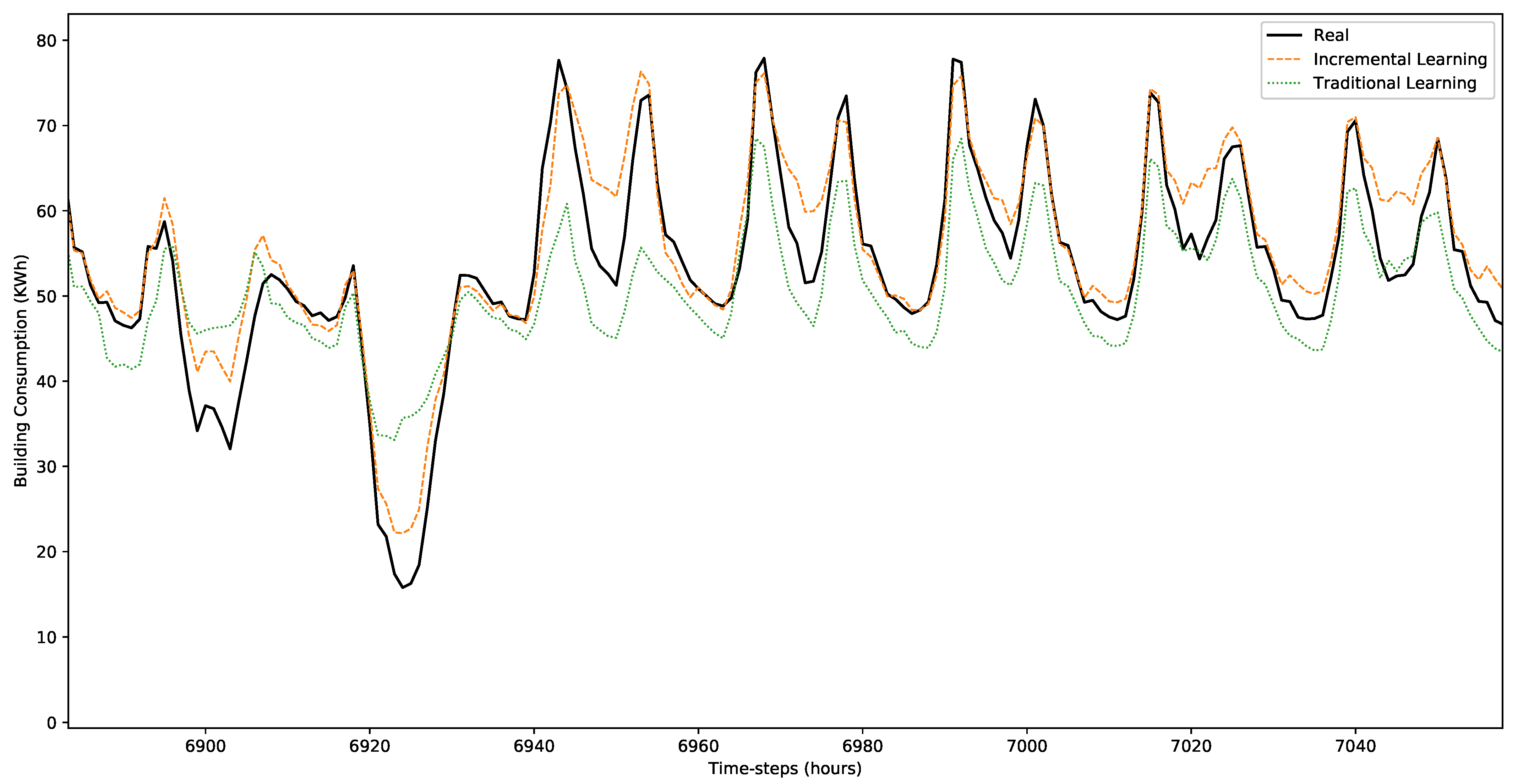
4.3. Results and Discussion
5. Conclusions
Author Contributions
Funding
Conflicts of Interest
Abbreviations
| ACF | Auto-Correlation Function |
| ANN | Artificial Neural Network |
| ARIMA | Autoregressive Integrated Moving Average |
| DL | Deep Learning |
| DSO | Distribution System Operator |
| DWT | Discrete Wavelet Transform |
| EMD | Empirical Mode Decomposition |
| GHG | Greenhouse Gas |
| HVAC | Heating, Ventilation, Air-Conditioning |
| IoT | Internet of Things |
| MAE | Mean Absolute Error |
| ML | Machine Learning |
| MLP | Multilayer Perceptron |
| MQTT | MQ Telemetry Transport |
| NRMSE | Normalized Root Mean Squared Error |
| NWP | Numerical Weather Prediction |
| PV | Photovoltaic |
| RE-SOINN | Regression Enhanced Self-organizing Incremental Neural Network |
| RES | Renewable Energy Sources |
| RMSE | Root Mean Squared Error |
| RVFL | Random Vector Functional Link |
| SCADA | Supervisory Control And Data Acquisition |
| SVM | Support Vector Machine |
References
- Marino, D.L.; Amarasinghe, K.; Manic, M. Building energy load forecasting using deep neural networks. In Proceedings of the IECON 2016-42nd Annual Conference of the IEEE Industrial Electronics Society, Florence, Italy, 23–26 October 2016; IEEE: Piscataway, NJ, USA, 2016; pp. 7046–7051. [Google Scholar]
- Wang, H.; Lei, Z.; Zhang, X.; Zhou, B.; Peng, J. A review of deep learning for renewable energy forecasting. Energy Convers. Manag. 2019, 198, 111799. [Google Scholar] [CrossRef]
- Tang, L.; Wu, Y.; Yu, L. A randomized-algorithm-based decomposition-ensemble learning methodology for energy price forecasting. Energy 2018, 157, 526–538. [Google Scholar] [CrossRef]
- Hong, T.; Pinson, P.; Wang, Y.; Weron, R.; Yang, D.; Zareipour, H. Energy forecasting: A review and outlook. IEEE Open Access J. Power Energy 2020, 7, 376–388. [Google Scholar] [CrossRef]
- Coignard, J.; Janvier, M.; Debusschere, V.; Moreau, G.; Chollet, S.; Caire, R. Evaluating forecasting methods in the context of local energy communities. Int. J. Electr. Power Energy Syst. 2021, 131, 106956. [Google Scholar] [CrossRef]
- Deb, C.; Zhang, F.; Yang, J.; Lee, S.E.; Shah, K.W. A review on time series forecasting techniques for building energy consumption. Renew. Sustain. Energy Rev. 2017, 74, 902–924. [Google Scholar] [CrossRef]
- Henzel, J.; Wróbel, Ł.; Fice, M.; Sikora, M. Energy consumption forecasting for the digital-twin model of the building. Energies 2022, 15, 4318. [Google Scholar] [CrossRef]
- Sarmas, E.; Dimitropoulos, N.; Strompolas, S.; Mylona, Z.; Marinakis, V.; Giannadakis, A.; Romaios, A.; Doukas, H. A web-based Building Automation and Control Service. In Proceedings of the 2022 13th International Conference on Information, Intelligence, Systems & Applications (IISA), Corfu, Greece, 18–20 July 2022; IEEE: Piscataway, NJ, USA, 2022; pp. 1–6. [Google Scholar]
- Fitch-Roy, O.; Fairbrass, J. Negotiating the EU’s 2030 Climate and Energy Framework; Springer: Berlin/Heidelberg, Germany, 2018. [Google Scholar]
- Sweeney, C.; Bessa, R.J.; Browell, J.; Pinson, P. The future of forecasting for renewable energy. Wiley Interdiscip. Rev. Energy Environ. 2020, 9, e365. [Google Scholar] [CrossRef]
- IEA. Solar PV, Paris. 2022. Available online: https://www.iea.org/reports/solar-pv (accessed on 9 November 2022).
- Das, U.K.; Tey, K.S.; Seyedmahmoudian, M.; Mekhilef, S.; Idris, M.Y.I.; Van Deventer, W.; Horan, B.; Stojcevski, A. Forecasting of photovoltaic power generation and model optimization: A review. Renew. Sustain. Energy Rev. 2018, 81, 912–928. [Google Scholar] [CrossRef]
- Spiliotis, E.; Legaki, N.Z.; Assimakopoulos, V.; Doukas, H.; El Moursi, M.S. Tracking the performance of photovoltaic systems: A tool for minimising the risk of malfunctions and deterioration. IET Renew. Power Gener. 2018, 12, 815–822. [Google Scholar] [CrossRef]
- Ssekulima, E.B.; Anwar, M.B.; Al Hinai, A.; El Moursi, M.S. Wind speed and solar irradiance forecasting techniques for enhanced renewable energy integration with the grid: A review. IET Renew. Power Gener. 2016, 10, 885–989. [Google Scholar] [CrossRef]
- Ahmad, A.S.; Hassan, M.Y.; Abdullah, M.P.; Rahman, H.A.; Hussin, F.; Abdullah, H.; Saidur, R. A review on applications of ANN and SVM for building electrical energy consumption forecasting. Renew. Sustain. Energy Rev. 2014, 33, 102–109. [Google Scholar] [CrossRef]
- Ahmed, R.; Sreeram, V.; Mishra, Y.; Arif, M. A review and evaluation of the state-of-the-art in PV solar power forecasting: Techniques and optimization. Renew. Sustain. Energy Rev. 2020, 124, 109792. [Google Scholar]
- Mayer, M.J. Benefits of physical and machine learning hybridization for photovoltaic power forecasting. Renew. Sustain. Energy Rev. 2022, 168, 112772. [Google Scholar] [CrossRef]
- Fara, L.; Diaconu, A.; Craciunescu, D.; Fara, S. Forecasting of energy production for photovoltaic systems based on ARIMA and ANN advanced models. Int. J. Photoenergy 2021, 2021. [Google Scholar] [CrossRef]
- Hassan, M.A.; Khalil, A.; Kaseb, S.; Kassem, M. Exploring the potential of tree-based ensemble methods in solar radiation modeling. Appl. Energy 2017, 203, 897–916. [Google Scholar] [CrossRef]
- Shi, J.; Lee, W.J.; Liu, Y.; Yang, Y.; Wang, P. Forecasting power output of photovoltaic systems based on weather classification and support vector machines. IEEE Trans. Ind. Appl. 2012, 48, 1064–1069. [Google Scholar] [CrossRef]
- Pazikadin, A.R.; Rifai, D.; Ali, K.; Malik, M.Z.; Abdalla, A.N.; Faraj, M.A. Solar irradiance measurement instrumentation and power solar generation forecasting based on Artificial Neural Networks (ANN): A review of five years research trend. Sci. Total Environ. 2020, 715, 136848. [Google Scholar] [CrossRef]
- Li, P.; Zhou, K.; Lu, X.; Yang, S. A hybrid deep learning model for short-term PV power forecasting. Appl. Energy 2020, 259, 114216. [Google Scholar] [CrossRef]
- Sarmas, E.; Spiliotis, E.; Marinakis, V.; Tzanes, G.; Kaldellis, J.K.; Doukas, H. ML-based energy management of water pumping systems for the application of peak shaving in small-scale islands. Sustain. Cities Soc. 2022, 82, 103873. [Google Scholar] [CrossRef]
- Zang, H.; Cheng, L.; Ding, T.; Cheung, K.W.; Wei, Z.; Sun, G. Day-ahead photovoltaic power forecasting approach based on deep convolutional neural networks and meta learning. Int. J. Electr. Power Energy Syst. 2020, 118, 105790. [Google Scholar] [CrossRef]
- Sarmas, E.; Dimitropoulos, N.; Marinakis, V.; Mylona, Z.; Doukas, H. Transfer learning strategies for solar power forecasting under data scarcity. Sci. Rep. 2022, 12, 1–13. [Google Scholar] [CrossRef] [PubMed]
- De Giorgi, M.G.; Congedo, P.M.; Malvoni, M. Photovoltaic power forecasting using statistical methods: Impact of weather data. IET Sci. Meas. Technol. 2014, 8, 90–97. [Google Scholar] [CrossRef]
- Yu, T.C.; Chang, H.T. The forecast of the electrical energy generated by photovoltaic systems using neural network method. In Proceedings of the 2011 International Conference on Electric Information and Control Engineering, Wuhan, China, 15–17 April 2011; IEEE: Piscataway, NJ, USA, 2011; pp. 2758–2761. [Google Scholar]
- Raza, M.Q.; Nadarajah, M.; Ekanayake, C. On recent advances in PV output power forecast. Sol. Energy 2016, 136, 125–144. [Google Scholar] [CrossRef]
- Sun, X.; Zhang, T. Solar power prediction in smart grid based on NWP data and an improved boosting method. In Proceedings of the 2017 IEEE International Conference on Energy Internet (ICEI), Beijing, China, 17–21 April 2017; IEEE: Piscataway, NJ, USA, 2017; pp. 89–94. [Google Scholar]
- Akeiber, H.; Nejat, P.; Majid, M.Z.A.; Wahid, M.A.; Jomehzadeh, F.; Famileh, I.Z.; Calautit, J.K.; Hughes, B.R.; Zaki, S.A. A review on phase change material (PCM) for sustainable passive cooling in building envelopes. Renew. Sustain. Energy Rev. 2016, 60, 1470–1497. [Google Scholar] [CrossRef]
- Sarmas, E.; Marinakis, V.; Doukas, H. A data-driven multicriteria decision making tool for assessing investments in energy efficiency. Oper. Res. 2022, 22, 5597–5616. [Google Scholar] [CrossRef]
- Kwok, S.S.; Lee, E.W. A study of the importance of occupancy to building cooling load in prediction by intelligent approach. Energy Convers. Manag. 2011, 52, 2555–2564. [Google Scholar] [CrossRef]
- Suganthi, L.; Samuel, A.A. Energy models for demand forecasting—A review. Renew. Sustain. Energy Rev. 2012, 16, 1223–1240. [Google Scholar] [CrossRef]
- Amasyali, K.; El-Gohary, N.M. A review of data-driven building energy consumption prediction studies. Renew. Sustain. Energy Rev. 2018, 81, 1192–1205. [Google Scholar] [CrossRef]
- Li, Q.; Ren, P.; Meng, Q. Prediction model of annual energy consumption of residential buildings. In Proceedings of the 2010 International Conference on Advances in Energy Engineering, Beijing, China, 19–20 June 2010; IEEE: Piscataway, NJ, USA, 2010; pp. 223–226. [Google Scholar]
- Liu, D.; Chen, Q. Prediction of building lighting energy consumption based on support vector regression. In Proceedings of the 2013 9th Asian Control Conference (ASCC), Istanbul, Turkey, 23–26 June 2013; IEEE: Piscataway, NJ, USA, 2013; pp. 1–5. [Google Scholar]
- Borges, C.E.; Penya, Y.K.; Fernández, I.; Prieto, J.; Bretos, O. Assessing tolerance-based robust short-term load forecasting in buildings. Energies 2013, 6, 2110–2129. [Google Scholar] [CrossRef]
- Saadi, M.; Noor, M.T.; Imran, A.; Toor, W.T.; Mumtaz, S.; Wuttisittikulkij, L. IoT enabled quality of experience measurement for next generation networks in smart cities. Sustain. Cities Soc. 2020, 60, 102266. [Google Scholar] [CrossRef]
- Sarmas, E.; Spiliotis, E.; Marinakis, V.; Koutselis, T.; Doukas, H. A meta-learning classification model for supporting decisions on energy efficiency investments. Energy Build. 2022, 258, 111836. [Google Scholar] [CrossRef]
- Marinakis, V. Big data for energy management and energy-efficient buildings. Energies 2020, 13, 1555. [Google Scholar] [CrossRef]
- Bouchachia, A.; Gabrys, B.; Sahel, Z. Overview of some incremental learning algorithms. In Proceedings of the 2007 IEEE International Fuzzy Systems Conference, London, UK, 23–26 July 2007; IEEE: Piscataway, NJ, USA, 2007; pp. 1–6. [Google Scholar]
- Ksieniewicz, P.; Zyblewski, P. Stream-learn—Open-source Python library for difficult data stream batch analysis. Neurocomputing 2022, 478, 11–21. [Google Scholar] [CrossRef]
- Puah, B.K.; Chong, L.W.; Wong, Y.W.; Begam, K.; Khan, N.; Juman, M.A.; Rajkumar, R.K. A regression unsupervised incremental learning algorithm for solar irradiance prediction. Renew. Energy 2021, 164, 908–925. [Google Scholar] [CrossRef]
- Qiu, X.; Suganthan, P.N.; Amaratunga, G.A. Ensemble incremental learning random vector functional link network for short-term electric load forecasting. Knowl.-Based Syst. 2018, 145, 182–196. [Google Scholar] [CrossRef]
- Gardner, M.W.; Dorling, S. Artificial neural networks (the multilayer perceptron)—A review of applications in the atmospheric sciences. Atmos. Environ. 1998, 32, 2627–2636. [Google Scholar] [CrossRef]
- Bourlard, H.; Kamp, Y. Auto-association by multilayer perceptrons and singular value decomposition. Biol. Cybern. 1988, 59, 291–294. [Google Scholar] [CrossRef]
- Rumelhart, D.E.; Hinton, G.E.; Williams, R.J. Learning representations by back-propagating errors. Nature 1986, 323, 533–536. [Google Scholar] [CrossRef]
- Hornik, K.; Stinchcombe, M.; White, H. Multilayer feedforward networks are universal approximators. Neural Netw. 1989, 2, 359–366. [Google Scholar] [CrossRef]
- Bifet, A.; Gavalda, R.; Holmes, G.; Pfahringer, B. Machine Learning for Data Streams: With Practical Examples in MOA; MIT Press: Cambridge, MA, USA, 2018. [Google Scholar]
- Ratcliff, R. Connectionist models of recognition memory: Constraints imposed by learning and forgetting functions. Psychol. Rev. 1990, 97, 285. [Google Scholar] [CrossRef]
- Robins, A. Catastrophic forgetting, rehearsal and pseudorehearsal. Connect. Sci. 1995, 7, 123–146. [Google Scholar] [CrossRef]
- He, J.; Mao, R.; Shao, Z.; Zhu, F. Incremental Learning in Online Scenario. In Proceedings of the IEEE/CVF Conference on Computer Vision and Pattern Recognition (CVPR), Seattle, WA, USA, 16–19 June 2020. [Google Scholar]
- MQTT. Available online: https://docs.oasis-open.org/mqtt/mqtt/v5.0/mqtt-v5.0.html (accessed on 25 November 2022).
- Buitinck, L.; Louppe, G.; Blondel, M.; Pedregosa, F.; Mueller, A.; Grisel, O.; Niculae, V.; Prettenhofer, P.; Gramfort, A.; Grobler, J.; et al. API design for machine learning software: Experiences from the scikit-learn project. In Proceedings of the ECML PKDD Workshop: Languages for Data Mining and Machine Learning, Prague, Czech Republic, 23–27 September 2013; pp. 108–122. [Google Scholar]
- Pedregosa, F.; Varoquaux, G.; Gramfort, A.; Michel, V.; Thirion, B.; Grisel, O.; Blondel, M.; Prettenhofer, P.; Weiss, R.; Dubourg, V.; et al. Scikit-learn: Machine learning in Python. J. Mach. Learn. Res. 2011, 12, 2825–2830. [Google Scholar]
- Scitkit-Learn 6. Strategies to Scale Computationally: Bigger Data. Available online: https://scikit-learn.org/0.15/modules/scaling_strategies.html#strategies-to-scale-computationally-bigger-data (accessed on 3 November 2022).


| Measure | PV Production | Electricity Consumption |
|---|---|---|
| Number of Hidden Layers | 4 | 3 |
| Neurons per Layer | 641,286,432 | 6,412,832 |
| Learning Rate | 0.001 | 0.001 |
| Solver | adam | adam |
| Measure | Incremental Learning | Traditional Learning |
|---|---|---|
| MAE | 6.697 | 7.273 |
| RMSE | 13.260 | 14.340 |
| nRMSE | 0.527 | 0.570 |
| Measure | Incremental Learning | Traditional Learning |
|---|---|---|
| MAE | 8.082 | 9.048 |
| RMSE | 12.391 | 13.429 |
| nRMSE | 0.214 | 0.232 |
Publisher’s Note: MDPI stays neutral with regard to jurisdictional claims in published maps and institutional affiliations. |
© 2022 by the authors. Licensee MDPI, Basel, Switzerland. This article is an open access article distributed under the terms and conditions of the Creative Commons Attribution (CC BY) license (https://creativecommons.org/licenses/by/4.0/).
Share and Cite
Sarmas, E.; Strompolas, S.; Marinakis, V.; Santori, F.; Bucarelli, M.A.; Doukas, H. An Incremental Learning Framework for Photovoltaic Production and Load Forecasting in Energy Microgrids. Electronics 2022, 11, 3962. https://doi.org/10.3390/electronics11233962
Sarmas E, Strompolas S, Marinakis V, Santori F, Bucarelli MA, Doukas H. An Incremental Learning Framework for Photovoltaic Production and Load Forecasting in Energy Microgrids. Electronics. 2022; 11(23):3962. https://doi.org/10.3390/electronics11233962
Chicago/Turabian StyleSarmas, Elissaios, Sofoklis Strompolas, Vangelis Marinakis, Francesca Santori, Marco Antonio Bucarelli, and Haris Doukas. 2022. "An Incremental Learning Framework for Photovoltaic Production and Load Forecasting in Energy Microgrids" Electronics 11, no. 23: 3962. https://doi.org/10.3390/electronics11233962
APA StyleSarmas, E., Strompolas, S., Marinakis, V., Santori, F., Bucarelli, M. A., & Doukas, H. (2022). An Incremental Learning Framework for Photovoltaic Production and Load Forecasting in Energy Microgrids. Electronics, 11(23), 3962. https://doi.org/10.3390/electronics11233962