Abstract
The integral equation method is one of the most successful computational models for microwave devices or integrated circuits in planar layered media. However, the efficient and accurate evaluation of the associated Green’s function consisting of Sommerfeld integrals (SIs) is still a remaining challenge. To mitigate this difficulty, this work proposes a spatial domain rational function fitting technique (RFFT) for SIs so that the approximation accuracy is controllable. In conjunction with an adaptive sampling strategy, the proposed RFFT minimizes the orders of rational functions, and the resultant SI evaluation efficiency is optimized. In addition, we investigate the semi-analytical singularity treatment for the rational expression of SIs in method of moment (MoM) implementation. Extensive simulation of representative planar devices validates the correctness of the proposed method and demonstrates its superior performance over conventional SI approximation methods.
1. Introduction
Since their invention in the last century, microstrip circuits and antennas have become some of the most popular types of devices delivering electromagnetic energy and signals [1,2,3]. Operating from 100 MHz to 100 GHz, the original microstrip structure has now evolved into multiple layered planar configurations where thin metallization lies between the interface between two dielectric substrates [4]. In the era of 5G communication, such planar devices become more ubiquitous due to the inherent nature of integration and minimization for stratified structures [5].
Compared with volumetric discretization schemes such as the finite-difference time-domain (FDTD) [6] and finite element method (FEM) [7], the integral equation method discretizing only the metallization surfaces has had great success in modeling these planar microwave device because of its accuracy and efficiency [8,9,10,11]. With Green’s function consisting of Sommerfeld integrals (SIs) in planar layered media available, the integral equations are established for the true or equivalent currents on metallization patterns only, and the approximated truncation boundary condition is avoided. In the past decades, considerable efforts have been made to improve the accuracy and efficiency of the method of moment (MoM) that solves these integral equations numerically. Generally, the efforts to fasciate the popularity of integral equations methods can be categorized into three kinds: (a) the integral equation formulations with higher accuracy or lower complexity in numerical implementation, (b) dedicated strategies to accelerate numerical discretization of integral equation, i.e., filling the impedance matrix, and (c) fast solvers for the matrix equation so electrically large or complicated structures can be efficiently simulated.
Unlike the free-space case, the optimal formulation for the integral equation in the planar layered medium is not unique because the scalar potential caused by horizontal and vertical dipoles are different [12]. To avoid the hypersingular behavior in the integral equation that cause difficulties in numerical implementation, three mixed-potential integral equation (MPIE) formulations (noted as A, B, and C) with singular weakly kernels were proposed [13], and formulation C was widely used in later studies because of its convenience in modeling targets penetrating dielectric interface. Later on, modified or extended MPIE formulations with improved numerical performance were developed for various applications at hand [9,14]. For instance, to overcome the low-frequency breakdown problem and support wideband simulation, the argument electric field integral equation (A-EFIE) [14] and current and charge integral equation (CCIE) [15] were developed. Most recently, a non-Galkerin quasi-MPIE formulation was proposed for efficient scattering analysis of homogeneous dielectric targets in a layered medium [16].
In a layered medium, Green’s function does not have a closed-form expression and is written as a tensor consisting of infinite integrals, also known as Sommerfeld integrals (SIs). Due to the slow decaying and oscillating kernel of SIs, the partition and then summation numerical integration for SIs is time-consuming. This causes the discretization of integral equations (i.e., the efficient filling of impedance matrix) has been a long-term numerical challenge that limits the performance of MoM when simulating planar circuits or antennas. To accelerate the convergence of numerical integration, extrapolation techniques such as weighted averages methods and double exponent quadrature were developed [17,18]. On the other hand, the closed-form approximation to SIs provides a faster solution in terms of calculation efficiency, and representative methods of this kind include the discrete complex image methods [19,20] and rational function fitting technique [21]. With improved robustness and accuracy in recent years, the unpredictable accuracy and numerical instability issue of closed-form approximation methods still remain to be addressed [5]. Compromise strategies between evaluation efficiency and the accuracy of SIs include the use of interpolation techniques [22] and the tailored DCIM method [23], where the accuracy of SI evaluation is firstly refined before the MoM procedure. However, due to the singularities in the layered Green’s function changing dramatically in the near-field region, a robust interpolation scheme with moderate sampling density is still challenging.
Besides the efforts with SI evaluation, another kind of approach to accelerate the filling of the impedance matrix is to adopt proper basis functions or integration methods to reduce the computational overload when evaluating the relevant reaction integrals. For example, based on DCIM, the analytical expression for evaluating double integrals for planar microstrip geometries is derived in [24] to avoid the double 2D integration. Furthermore, studies show that the double 2D integration can be transformed into a quasi-1D integration in a more general multilayer medium, which further decreases simulation time [10]. With the development of modern computation architecture, parallel computation techniques such as graphic processing units (GPU) are also considered to accelerate the MPIE simulations in recent years [11].
As any progress in SI evaluation techniques will directly result in faster and more accurate simulation tools for circuits and antennas in layered medium, in this work, we consider a closed-form rational function fitting technique (RFFT) for SIs. To minimize the order’s RFFT expression with a controllable accuracy, an adaptive sampling procedure is proposed for a given spatial region of interest. In addition, a semi-analytical scheme to evaluate impedance matrix elements with a nearly singular kernel is presented to alleviate calculation difficulties in numerical integration.
The rest of the paper is organized as follows. In Section 2, after a brief introduction to MPIE formulation, the adaptive RFFT for SIs in Green’s function is presented and verified. The Duffy transform to handle near-singular integration based on the rational expression is derived in the second subsection. Numerical results and comparisons for planar circuits and antennas in multilayer medium are presented in Section 3 to demonstrate the effectiveness of the proposed methods. Finally, conclusions and some remarks are given in Section 4.
2. Theory and Formulations
Before beginning the discussion of the proposed methods in this work, we first briefly introduce the problem addressed in this work, the associated MPIE formulation, and its MoM discretization. In this work, the efficient electromagnetic analysis of RF circuits or devices in a multilayer planar medium is considered, as illustrated in Figure 1, where the material discontinuity lies only in z axis of the Cartesian -coordinate system. The dielectric layers from up to down are denoted as layer with a permittivity and permeability of . Here, we assume the time dependence, and that the metallic circuit or devices are thin perfectly conducting sheets lying between the interface between different media. Such structures can be found in various modern radio frequency devices such as antennas, filters, and couplers because of the inherent nature of the integration of planar structures.
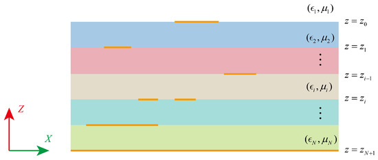
Figure 1.
Illustration of the electromagnetic problem in multilayered media.
Simplifying the metallization patterns in the planar layered medium as perfectly conducting sheets and following the most popular MPIE formulation [13], the unknown electric current on the metallic surfaces satisfy the following equation:
where denotes the surface of S in the layer, and is the unit vector normal to . The magnetic vector potential and scalar potential in layer caused by electrical currents or charges in layer are expressed as
where q is the surface charge density and . The vector potential Green’s function takes the form
The entries of and scalar potential Green’s function are all Sommerfeld integrals and have a general form of
where is the zero-order Bessel function, and is the horizontal distance between source point and field point . In (5), is denoted as the spectral domain Green’s function, and is calculated by using the transmission line theory [13].
Applying the Galerkin testing procedure, the MPIE can be discretized into a matrix equation , is the right-hand-side vector based on the excitation on circuit, and is the unknown vector relating to the unknown currents by basis functions. The entries of impedance matrix are given by
where and are the basis and testing functions defined in mesh unit and , respectively.
2.1. Proposed Adaptive RFFT
In the previous studies, the RFF methods are usually first performed in the spectral domain to approximate the SI integrands, i.e., in Equation (5), then the closed-form expressions using integral identities are obtained. Unfortunately, spatial accuracy of such treatment is somehow difficult to evaluate or control in practical applications [25].
To achieve an accuracy-controllable closed-form approximation, we considered the rational fitting function (RFF) directly in the spatial domain. After extracting poles and quasi-static terms in original SIs, for a given and z, the remaining SI is approximated by a piecewise rational function, and given as
and is a threshold horizontal distance separating the singular and regular behavior of SIs, and it takes the value of one dielectric wavelength from our empirical studies. The reason for choosing RFF here is based on the following considerations. First, the RF approximation is well known for producing an excellent local approximation to arbitrary functions. Secondly, evaluating rational functions is generally more efficient than the existing closed-form approximation scheme to a Sommerfeld integral that contains the Hankel function or other special functions. In addition, we find that RFF expression facilitates the efficient evaluation of MoM impedance entries, as explained later in this paper.
Although an unified RFF model can be established to approximate with satisfying accuracy, we found that the piecewise approximation in (7) is much faster in terms of numerical calculation. As the metallization pattern lies only on the interface between different dielectric layers, only a finite amount of discrete z and values need to be evaluated in MoM simulations.
Both and in (7) are written by the rational function as follows:
where is a polynomial function with order n. Here, superscript in the above notation is omitted for simplicity. To find the lowest order of polynomials and their associated unknown coefficients in (8) with a preset accuracy, an iterative procedure is illustrated in Algorithm 1, shown below. The fundamental idea here is to use two RFF models to approximate the SI in the spatial domain, and the additional sampling point for improving the approximation accuracy is determined by the discrepancy between these two models
This iterative procedure continues until the relative error between these two models is lower than the preset threshold . The proposed algorithm is summarized in Algorithm 1, and the rational function orders updating paths for the two models are presented in Figure 2. Clearly, the order updating paths shown in this diagram cover larger subsets of combinations and hence yields a better fitting performance. In this algorithm, the Bulirsch–Stoer (BS) algorithm [26] is recommended for the robust and efficient evaluating or updating of unknown coefficients in an RFF model (8). Combing the Richardson extrapolation and modified midpoint method, the BS algorithm finds the numerical solution of RFF or ordinary differential equations with a high accuracy and relatively low computational complexity, and its numerical implementation can be found in the well-known literature (chapter 3.4) [27].
| Algorithm 1: Adaptive RFF for SIs |
 |
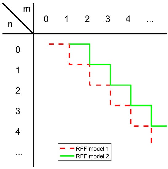
Figure 2.
Order updating path of different RFF models in Algorithm 1.
To verify the performance of the proposed adaptive RFFT, the CPU time to obtain approximation parameters, SIs evaluation time, and the approximation accuracy are presented in Table 1 and Table 2 for two configurations of layered media. Although there are more advanced DCIM schemes available [25], here we use the classic two-level DCIM scheme [20] as the benchmark for comparison as the resultant number of complex images is moderate and approximation accuracy is decent for the examined spatial region after removing quasi-static terms. The approximation accuracy here is calculated by comparing the results between closed-form schemes and the numerical integration method [17].

Table 1.
Performance comparison for different SI approximation methods for a microstrip structure.
Table 2.
Performance comparison for different SI approximation methods for a four-layer stacked medium.
In Table 1, the SIs in and are evaluated and compared for a microstrip structure with a dielectric constant of and a thickness of , while in Table 2, a two-layer PEC-backed dielectric substrate with a thickness of , 0.1 is considered, and their dielectric constants are j and j, respectively. From these two tables, we can see that the calculation time to establish closed-form expressions is a few times larger than the counterpart of DCIM. Nevertheless, it is still a neglectable portion compared to the numerical evaluation of SIs. The typical convergence history of the proposed adaptive RFFT is shown in Figure 3, where the preset accuracy is set to be . Although the orders of polynomials in RFFs are comparable to the number of complex images in two-level DCIM, the proposed method provides a speed increase of ten to twenty times, and more importantly it has a higher approximation accuracy.
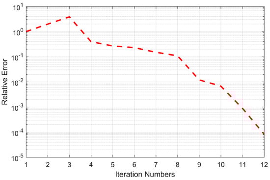
Figure 3.
Typical convergence behavior of the proposed adaptive RFFT.
2.2. Singularity Treatment
Besides the efficient SI evaluation, the fast calculation of the impedance matrix elements based on the proposed closed-form expression is also considered. For the sake of efficient calculation and convenience of singularity analysis, by finding the roots of the denominator, the rational function expression in (7) is rewritten as the sum of the simple rational functions that follow:
Substituting (10) into (6), there are two elementary integrals to be evaluated
where is the free vertex of the RWG basis function. Clearly, the magnitude is nearly zero when the associated SI is nearly singular, hence the numerical integration of (6) can be time-consuming when the horizontal distance between and is close to zero.
To overcome this difficulty in numerical integration, we consider the Duffy transformation technique [28]. Let be a triangle associated with a basis function with tree vertices , , and , as shown in Figure 4a, and is the vector of field point project to plane . The integration domain can be divided into three sub-triangles and using the addition vertex . In the Duffy transformation, take as an example. It can be mapped into a transformed domain, as shown in Figure 4b,c, and given by
where scalars and are
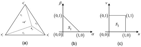
Figure 4.
Duffy transformation for triangles, (a) coordinates of the integration triangle, (b) mapping to a standard triangle and (c) mapping to a standard rectangle.
In this way, the integrals in (11) can be rewritten as the summation of three singularity-free integrals on and , i.e., and . For the integral on we have
where , , , and is the area of . The rest of the integrals on and have identical forms except for the different vector definition and their expressions are omitted here for brevity.
Observing the integrals on sub-triangles shown in (14), we find that only three types of integration are required to be evaluated here.
Fortunately, analytical expressions are available for double integral (15b) and (15c) and given in Appendix A. The integral in (15a) can be converted to a one-dimensional integral by eliminating u
The first two terms in (16) also have analytical expressions and are presented in Appendix A. The third term in (16) generally does not have an analytical expression, depends on the position of , and the evaluation strategy may differ.
- If lies on the direction vector , i.e., , we can define scalar , and the integral can be analytically evaluated. The detailed expressions given in Appendix B depend on the value of p.
- If is far from vector , the above integral has to be evaluated numerically using adaptive Gaussian integration.
- If is close to vector but not lies on it, to avoid the numerical integration for almost singular integrand as approx to zero, here we use the approximated conditionthen derive the approximated analytical expression for as shown in Appendix B.
In addition, for the special case where coincide with or , the analytical expressions for above three integrals in (15) are derived in Appendix C.
To verify the validity of the semi-analytical strategy to evaluate integral (15a), here we examined the performance of the proposed method in two extreme cases. As shown in Figure 5, the required number of Gaussian quadrature points to achieve the relative error is less than . In this figure, lengths are normalized by the average length of the source triangle edge length, and the triangle edges are illustrated by black lines in plane. The vector relating to the field point varies in the range and , and the number of required points are represented by the color of each pixel. Obviously, around two or three Gaussian points are sufficient to achieve good accuracy when is far from the source triangle, even though is quite small. More Gaussian points are required when is located near the triangle edges. Nevertheless, the use of approximation (17) makes the maximum number of Gaussian points still below 20.
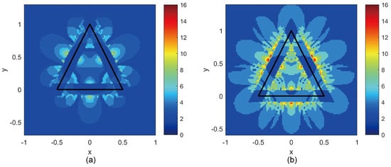
Figure 5.
Number of Gaussian quadrature points required for evaluation (15a) in extreme cases (a) , (b) .
3. Numerical Validation
In this section, based on the MoM analysis of planar structures in microwave engineering, numerical examples to demonstrate the calculation efficiency of the proposed method are presented through comparisons.
3.1. A Microstrip Low-Pass Filter
We first considered an MoM simulation of a microstrip-design low-pass filter to verify the correctness and efficiency of the proposed SI evaluation technique and the singularity treatment strategy. The microstrip structure is identical to the aforementioned one whose SIs evaluation performance is compared in Table 1. The metallization pattern is printed on top of the substrate surface and shown in Figure 6, with two ports at the front and end of this structure, the simulated S11 and S12 parameters are presented in Figure 7a,b, respectively. This low-pass filter has a length of around 46 mm, a width of around 16.93 mm, and the dielectric substrate length is 0.254 mm. Due to the reciprocity of this device, S22 and S21 parameters are omitted here for simplicity. In addition, here we also presented the S-parameter results evaluated by MoM using DCIM and by a commercial MoM tool FEKO in the same plot. In Figure 7, a good agreement between these three methods can be observed, except for S12 at the stopband where the value is lower than −50 dB, which is extremely sensitive to round-off errors in numerical calculation. To verify this point, at 2.9 GHz where the S12 has around 10 dB discrepancy between different methods, the surface current intensity of the LPF circuit by excitation port 2 with a voltage source is presented in Figure 8. The current intensity near port 1 almost vanished to zero in all three simulations, as the operation frequency is located in the stopband of this LPF. The electric current intensity plots are also almost identical and indicate the correctness and accuracy of the proposed method, despite the fact that the S21 error is large here.
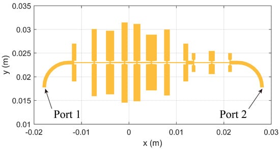
Figure 6.
Metallization pattern of a microstrip two−port low−pass filter.
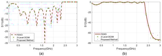
Figure 7.
S−parameter of the two-port low-pass filter evaluated by different methods, (a) S11, and (b) S12.
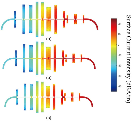
Figure 8.
Surface current intensity of LPF at 2.9 GHz for voltage excitation on port 2 at 2.9 GHz calculated by different methods, (a) FEKO, (b) 2−Level DCIM and (c) the proposed method.
In addition to the S-parameter curves, the MoM calculation CPU time using different SI evaluation schemes is presented in Table 3 for comparison. In particular, we also provide the CPU time for filling the impedance matrix in the MoM procedure in the second and fourth columns of this table. Clearly, without losing simulation accuracy, compared to two-level DCIM, the proposed method has an increase in speed of approximately in terms of total calculation time and a larger increase in speed in terms of filling the impedance matrix.
Table 3.
Calculation CPU Time (s) for different planar structures using MoM.
3.2. A Stacked Antenna
The following example considers a stacked planar antenna simulation using MoM and layered Green’s function. The layered medium configuration is shown in Figure 9a, where an additional infinite thin metallization (shown in blue) sheet is inserted into the dielectric substrate and connected to the feeding pin; we treated this layered medium as a four-layered structure. The layout of this antenna design is shown in Figure 9b, where the four rectangular sheets shown in red in this figure are printed on top of the dielectric substrate and act as radiation elements in this antenna design so that an omnidirectional radiation pattern can be achieved. Using the microstrip edge port as excitation, the input impedance and radiation pattern of this antenna with infinitely large ground and substrate can be efficiently simulated.
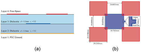
Figure 9.
A stacked antenna, (a) layered medium configuration, (b) antenna metallization geometry.
Similar to the previous numerical example, the input impedance of this antenna is calculated by MoM with different SI evaluation schemes, i.e., the proposed methods and the conventional two-level DCIM. The input impedance values in the frequency band from 1.6 GHz to 3.2 GHz with 50 MHz interval are presented in Figure 10, where the resistance and reactance are plotted in Figure 10a,b. Again, a very good agreement between the different methods in calculating the input impedance of this antenna can be observed in the examined frequency band. The CPU time comparisons for total computational time and time taken for filling the impedance matrix are also provided in Table 3. Again, an approximately seven times increase in speed of can be seen in this example.
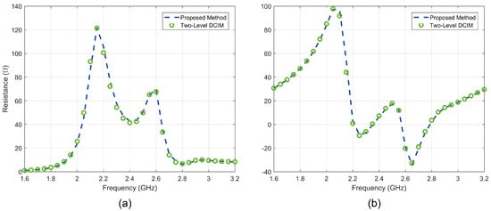
Figure 10.
Input impedance of the stacked antenna simulated by different methods (a) resistance, (b) reactance.
4. Conclusions
Aiming for a more efficient MoM simulation for planar circuits and antennas, the fast closed-form evaluation of SIs in the layered medium is considered in this work. Using the rational function approximation to SIs directly in the spatial domain, the proposed adaptive RFFT achieves fast evaluation of SIs with a preset approximation accuracy. In addition, the semi-analytical expressions for the near-singular SIs in MoM implementation are derived and verified based on the proposed RFFT. Representative MoM simulations for planar devices in microwave engineering are studied to demonstrate the correctness and efficiency of the proposed methods and an increase in speed of several times can be achieved when compared to classic DCIM. As an adaptive fitting technique for SIs, the proposed method is robust and flexible in the approximation of Green’s function in an arbitrary layered medium without considering the vertical location of source and field points. Hence, it can be integrated into existing MoM tools easily to accelerate the electromagnetic analysis of planar circuits and antennas.
Author Contributions
Conceptualization and investigation, Z.-H.Z., Z.-L.L., B.-Y.W., M.-L.Y. and X.-Q.S.; methodology, Z.-H.Z., Z.-L.L., B.-Y.W.; software, Z.-L.L. and M.-L.Y.; validation, B.-Y.W., M.-L.Y. and X.-Q.S.; writing, Z.-H.Z. and B.-Y.W.; formal analysis, M.-L.Y. and X.-Q.S.; data curation, Z.-H.Z.; supervision, X.-Q.S.; project administration, X.-Q.S.; funding acquisition, B.-Y.W. and X.-Q.S. All authors have read and agreed to the published version of the manuscript.
Funding
This work was supported in part by the National Natural Science Foundation of China (NSFC) under Grant No. 62271046 and the Young Elite Scientist Scholarship program of the China Association for Science and Technology(CAST) grant No. 2020QNRC001.
Data Availability Statement
Not applicable.
Acknowledgments
The authors would like to thank the anonymous reviewers for their valuable comments.
Conflicts of Interest
The authors declare no conflict of interest.
Appendix A
The analytical expression for integrals in (15) are given as follow
where function is defined as
The analytical expression for the first two terms in (16) can be calculated using the following identity.
The coefficients are defined as follow. Among them only , , and are related to the value of in RFF expression to SIs, the rest are determined by the source triangle vertexes and vector , and the scalar are the length of vector
Appendix B
Substituting into the integrand of (15a), we have
then analytical expressions for can be derived base on the value of p. If or , then
If , then
Appendix C
If coincides with or , the analytical expressions in Appendices Appendix A and Appendix B are rewritten as follows
and
If , then
if ,
References
- Garg, R.; Bhartia, P.; Bahl, I.J.; Ittipiboon, A. Microstrip Antenna Design Handbook; Artech House: Norwood, MA, USA, 2001. [Google Scholar]
- Peixeiro, C. Microstrip patch antennas: An historical perspective of the development. In Proceedings of the 2011 SBMO/IEEE MTT-S International Microwave and Optoelectronics Conference (IMOC 2011), Natal, Brazil, 29 October–1 November 2011; pp. 684–688. [Google Scholar]
- Edwards, T.C.; Steer, M.B. Foundations for Microstrip Circuit Design; John Wiley & Sons: Hoboken, NJ, USA, 2016. [Google Scholar]
- MOSIG, J.R.; MICHALSKI, K.A. Sommerfeld integrals and their relation to the development of planar microwave devices. IEEE J. Microwaves 2021, 1, 470–480. [Google Scholar] [CrossRef]
- Mittra, R.; Ozgun, O.; Li, C.; Kuzuoglu, M. Efficient Computation of Green’s Functions for Multilayer Media in the Context of 5G Applications. In Proceedings of the 2021 15th European Conference on Antennas and Propagation (EuCAP), Dusseldorf, Germany, 22–26 March 2021; pp. 1–5. [Google Scholar]
- Winton, S.C.; Kosmas, P.; Rappaport, C.M. FDTD simulation of TE and TM plane waves at nonzero incidence in arbitrary layered media. IEEE Trans. Antennas Propag. 2005, 53, 1721–1728. [Google Scholar] [CrossRef]
- Zhang, K.; Goddard, L.L.; Jin, J.M. Efficient large-scale scattering analysis of objects in a stratified medium. Int. J. Numer. Model. Electron. Netw. Devices Fields 2020, 33, e2656. [Google Scholar] [CrossRef]
- Sercu, J.; Fache, N.; Libbrecht, F.; Lagasse, P. Mixed potential integral equation technique for hybrid microstrip-slotline multilayered circuits using a mixed rectangular-triangular mesh. IEEE Trans. Microw. Theory Tech. 1995, 43, 1162–1172. [Google Scholar] [CrossRef]
- Michalski, K.A.; Mosig, J.R. Multilayered media Green’s functions in integral equation formulations. IEEE Trans. Antennas Propag. 1997, 45, 508–519. [Google Scholar] [CrossRef]
- Tarricone, L.; Mongiardo, M.; Cervelli, F. A quasi-one-dimensional integration technique for the analysis of planar microstrip circuits via MPIE/MoM. IEEE Trans. Microw. Theory Tech. 2001, 49, 517–523. [Google Scholar] [CrossRef]
- De Donno, D.; Esposito, A.; Monti, G.; Tarricone, L. MPIE/MoM acceleration with a general-purpose graphics processing unit. IEEE Trans. Microw. Theory Tech. 2012, 60, 2693–2701. [Google Scholar] [CrossRef]
- Michalski, K.A. On the scalar potential of a point charge associated with a time-harmonic dipole in a layered medium. IEEE Trans. Antennas Propag. 1987, 35, 1299–1301. [Google Scholar] [CrossRef]
- Michalski, K.A.; Zheng, D. Electromagnetic scattering and radiation by surfaces of arbitrary shape in layered media. I. Theory. IEEE Trans. Antennas Propag. 1990, 38, 335–344. [Google Scholar] [CrossRef]
- Chen, Y.P.; Jiang, L.; Qian, Z.G.; Chew, W.C. An augmented electric field integral equation for layered medium Green’s function. IEEE Trans. Antennas Propag. 2010, 59, 960–968. [Google Scholar] [CrossRef]
- Ren, Y.; Zhao, S.W.; Chen, Y.; Hong, D.; Liu, Q.H. Simulation of Low-Frequency Scattering From Penetrable Objects in Layered Medium by Current and Charge Integral Equations. IEEE Trans. Geosci. Remote. Sens. 2018, 56, 6537–6546. [Google Scholar] [CrossRef]
- Ren, Y.; Zhao, X.; Lin, Z.; Chen, Y.; Meng, M.; Liu, Y.; Zhao, H. A Quasi-Mixed-Potential Layered Medium Green’s Function for Non-Galerkin Surface Integral Equation Formulations. IEEE Trans. Antennas Propag. 2022, 70, 2070–2081. [Google Scholar] [CrossRef]
- Michalski, K.A. Extrapolation methods for Sommerfeld integral tails. IEEE Trans. Antennas Propag. 1998, 46, 1405–1418. [Google Scholar] [CrossRef]
- Michalski, K.A.; Mosig, J.R. Efficient computation of Sommerfeld integral tails–methods and algorithms. J. Electromagn. Waves Appl. 2016, 30, 281–317. [Google Scholar] [CrossRef]
- Fang, D.; Yang, J.; Delisle, G. Discrete image theory for horizontal electric dipoles in a multilayered medium. In Proceedings of the IEE Proceedings H-Microwaves, Antennas and Propagation; IET: Stevenage, UK, 1988; Volume 135, pp. 297–303. [Google Scholar]
- Dural, G.; Aksun, M.I. Closed-form Green’s functions for general sources and stratified media. IEEE Trans. Microw. Theory Tech. 1995, 43, 1545–1552. [Google Scholar] [CrossRef]
- Okhmatovski, V.I.; Cangellaris, A.C. Evaluation of layered media Green’s functions via rational function fitting. IEEE Microw. Wirel. Components Lett. 2004, 14, 22–24. [Google Scholar] [CrossRef]
- Valerio, G.; Baccarelli, P.; Paulotto, S.; Frezza, F.; Galli, A. Regularization of mixed-potential layered-media Green’s functions for efficient interpolation procedures in planar periodic structures. IEEE Trans. Antennas Propag. 2009, 57, 122–134. [Google Scholar] [CrossRef]
- Wu, B.Y.; Sheng, X.Q. A complex image reduction technique using genetic algorithm for the MoM solution of half-space MPIE. IEEE Trans. Antennas Propag. 2015, 63, 3727–3731. [Google Scholar] [CrossRef]
- Alatan, L.; Aksun, M.; Mahadevan, K.; Birand, M.T. Analytical evaluation of the MoM matrix elements. IEEE Trans. Microw. Theory Tech. 1996, 44, 519–525. [Google Scholar] [CrossRef]
- Alparslan, A.; Aksun, M.I.; Michalski, K.A. Closed-form Green’s functions in planar layered media for all ranges and materials. IEEE Trans. Microw. Theory Tech. 2010, 58, 602–613. [Google Scholar] [CrossRef]
- Stoer, R.B.J. Introduction to Numerical Analysis, 3rd ed.; Texts in Applied Mathematics 12; Springer: New York, NY, USA, 2002. [Google Scholar]
- Press, W.H.; Teukolsky, S.A.; Vetterling, W.T.; Flannery, B.P. Numerical Recipes: The Art of Scientific Computing, 3rd ed.; Cambridge University Press: Cambridge, UK, 2007. [Google Scholar]
- Khayat, M.A.; Wilton, D.R. Numerical evaluation of singular and near-singular potential integrals. IEEE Trans. Antennas Propag. 2005, 53, 3180–3190. [Google Scholar] [CrossRef]
Publisher’s Note: MDPI stays neutral with regard to jurisdictional claims in published maps and institutional affiliations. |
© 2022 by the authors. Licensee MDPI, Basel, Switzerland. This article is an open access article distributed under the terms and conditions of the Creative Commons Attribution (CC BY) license (https://creativecommons.org/licenses/by/4.0/).