Article

An Adaptive Beetle Swarm Optimization Algorithm with Novel Opposition-Based Learning

School of Computer and Information Engineering, Jiangxi Agricultural University, Nanchang 330045, China
*
Author to whom correspondence should be addressed.
Electronics 2022, 11(23), 3905; https://doi.org/10.3390/electronics11233905
Submission received: 31 October 2022 / Revised: 23 November 2022 / Accepted: 23 November 2022 / Published: 25 November 2022
(This article belongs to the Section Artificial Intelligence)

Abstract

:
The Beetle Swarm Optimization (BSO) algorithm is a high-performance swarm intelligent algorithm based on beetle behaviors. However, it suffers from poor search speeds and is prone to local optimization due to the size of the step length. To address this further, a novel improved opposition-based learning mechanism is utilized, and an adaptive beetle swarm optimization algorithm with novel opposition-based learning (NOBBSO) is proposed. In the proposed NOBBSO algorithm, the novel opposition-based learning is designed as follows. Firstly, according to the characteristics of the swarm intelligence algorithms, a new opposite solution is obtained to generate the current optimal solution by iterations in the current population. The novel opposition-based learning strategy is easy to converge quickly. Secondly, an adaptive strategy is used to make NOBBSO parameters self-adaptive, which makes the results tend to converge more easily. Finally, 27 CEC2017 benchmark functions are tested to verify its effectiveness. Comprehensive numerical experiment outcomes demonstrate that the NOBBSO algorithm has obtained faster convergent speed and higher convergent accuracy in comparison with other outstanding competitors.

1. Introduction

Swarm-based intelligent algorithms have been developed to address complicated nonlinear optimization problems more and more in recent years. The reason for this is that there is a variety of optimization problems in engineering which are difficult to be solved effectively in a limited time using traditional optimization methods, and hence it has been one of important research hotspots. Swarm intelligent (SI) algorithms are stochastic search methods which can deal with optimization issues successfully. SI algorithms are designed based on natural occurrences and have been proved to be more excellent in addressing optimization issues than standard algorithms in many cases such as particle swarm algorithm (PSO) [1] developed via mimicking the motion behavior of birds, artificial bee swarm algorithm (ABC) [2] developed based on the forging of bees, ant colony algorithm [3] developed on the basis of the motion of ants and beetle swarm algorithm created based on the movement of beetle swarm.
Beetle swarm optimization (BSO) [4] is a novel swarm intelligent algorithm based on beetle group behavior. Some studies demonstrate that it performs better than previous intelligence algorithms in accuracy and convergence speed. Hence it is a very successful algorithm for addressing optimization problems. Moreover, the algorithm has been widely used in the optimization problems of various disciplines. For example, Wang et al. [5] put forward the improved BSO algorithm based on new trajectory planning and used the algorithm for trajectory planning of robot manipulators. Hariharan et al. [6] mixed PSO and BSO algorithms to propose an adaptive BSO algorithm and applied it to improve BSO algorithm to solve the energy-efficient multi-objective virtual machine integration. Since the search strategy of BSO algorithm is better than PSO algorithm, Mu et al. [7] applied it on top of 3D route planning. Singh et al. [8] combined BSO algorithm to propose a heart disease and multi morbidity diagnosis model. Jiang et al. [9] utilized the efficiency of BSO algorithm to localize and quantify structural damage. Zhou et al. [10] put forward an improved BSO algorithm to obtain the shortest path and implementing intelligent navigation control for autonomous navigation robots. Zhang et al. [11] proposed a novel gait multi-objectives optimization strategy based on beetle swarm optimization to solve the lower limb exoskeleton robot.
However, the BSO algorithm still has some drawbacks. When a beetle falls into a local optimal solution, other beetles can gather to the beetle. It tends to make the algorithm skip the global optimal solution, and thus sinks into a local optimal solution. This study proposes a novel improved opposition-based learning method which is more suitable for swarm intelligence algorithms, and it is illustrated in detail in the subsequent Section 3.1 of the study. The original opposition-based learning [12] is an effective intelligent optimization strategy with extensive practical applications, such as the improved particle swarm algorithm [13] that uses opposition-based learning. However, the optimization performance of the opposition-based learning strategy is not so good in the later phase of iterations, so that some variations of the opposition-based learning algorithm have emerged such as the refraction opposition-based learning model based on refraction principle [14] and the elite opposition-based learning [15,16,17].
Therefore, in this study, a novel opposition-based learning method is proposed to enhance the performance of the original opposition-based learning. In addition, an adaptive strategy is proposed to achieve a better balance on the selection between the BSO algorithm and particle swarm algorithm to enhance its optimization. In the future, the proposed algorithm can be used to solve engineering problems to verify its performance, such as a robust fuzzy control approach for path-following control of autonomous vehicles [18].
The remainder of the study is constructed as below. Firstly, Section 2 demonstrates the related work of this study including the beetle swarm algorithm and the opposition-based learning. After that, the design of the NOBBSO algorithm is presented in Section 3, which includes the utilization of the opposition-based learning in the algorithm and an adaptive strategy is proposed. Section 4 analyzes the experiments, including parameter settings and test functions and convergence analysis. Section 5 discusses the merits and demerits of the NOBBSO algorithm. Finally, a summary is presented in Section 6.

2. Related Preparatory Knowledge

2.1. Beetle Swarm Optimization

2.1.1. Thought of Beetle Antennae Search

Beetle antennae search (BAS) [19] algorithm is a beetle behavior-based algorithm with the following basic idea: the two antennae of the beetle, like those of most insects, are its primary chemical receptors. Its antennae play a key role in helping it discover food by receiving up signals from its partners. When a signal is received by the antennae of the beetle, it compares the signal intensity between the two antennae and moves towards to the direction of the stronger signal.
Beetle and tentacle are regarded as particles based on their behaviors, and a mathematical model is developed for them. The random search direction of the beetle is formulated as the following Equation (1)
b = r a n d s ( n , 1 ) r a n d s ( n , 1 )
where b is the beetle search direction, and r a n d s ( ) denotes a random function. n denotes a point in that dimension.
The following is the relationship between the antenna and the beetle, which is represented by Equations (2) and (3).
x r t = x t + d t 2 b
x l t = x t d t 2 b
where x t denotes the position of the t-th generation, and d t represents the distance between the beetle and the antenna. x r t and x l t represent the positions of the right and left tentacles of beetles, respectively.
The movement of the beetle is then abstracted into the following Equation (4).
x t + 1 = x t + δ t b s i g n ( f ( x r t ) f ( x l t ) )
where δ t denotes the step size of the search of the beetle, and its value decreases as the numbers of searching increase. The term x t denotes the position of the beetle at the t-th generation. The term x t + 1 represents the position of the beetle at the next generation. The function s i g n ( ) denotes the symbolic function and the function f ( ) is used to calculate the signal condition at that instant.
The size of d t is fluctuated with the one of δ t in this process, which is formulated as the following Equations (5) and (6).
δ t + 1 = 0.95 δ t
d t = δ t c 2
where c 2 is a constant.

2.1.2. Beetle Swarm Optimization Principle

Beetle swarm optimization is an improved beetle antennae algorithm with better optimization performance. Because the BAS algorithm is not particularly expert in dealing with multi-dimensional functions, the creator of the BSO algorithm employs the idea of the swarm intelligent algorithm to improve its performance.
The general thought of the beetle swarm optimization algorithm is described as below. Beetles denote candidate solutions for a given optimization problem, and they can exchange their fitness information with each other in the same way as a particle swarm optimization algorithm does in the population. However, the distances and directions of beetles are governed by their speed and antenna information.
In mathematical terms, similar to the PSO algorithm, there are n beetles X = ( X 1 , X 2 , , X n ) in the searching space in the S dimension. The position information of the i-th beetle is expressed as X i = ( X i 1 , X i 2 , , X i s ) , and the velocity of the i-th beetle is expressed as V i = ( V i 1 , V i 2 , , V i s ) , and the optimal i-th beetle is expressed as P i = ( P i 1 , P i 2 , , P i s ) . The optimal beetle in a group of beetles is expressed as P g = ( P g 1 , P g 2 , , P g s ) . The movement of beetles is described as the following Equation (7).
X i s t + 1 = X i s t + λ V i s t + ( 1     λ ) ξ i s t
where the parameter s = 1 , 2 , S , i = 1 , 2 , , n , and t is the number of the current iteration, and V i s t represents the speed of the beetle, and ξ i s t represents the increment of the movement of the beetle. The parameter λ is a constant.
The velocity formula can be written as the following Equation (8).
V i s t + 1 = w V i s t + c 1 r 1 ( P i s t X i s t ) + c 2 r 2 ( P g s t X g s t )
where c 1 and c 2 are positive numbers. r 1 and r 2 are random numbers ranging from 0 to 1. w is a weight value which is an adaptive number with the following Equation (9).
w = w max w max w min T t
where w max and w min represent the maximum and minimum values respectively. The term t is the number of the current iteration, and T the number of the maximum iteration.
The above parameter ξ is defined as the following Equation (10).
ξ i s t + 1 = δ t V i s t s i g n ( f ( X r s t ) f ( X l s t ) )
where the parameter δ denotes the size of step, and the terms X r s t and X l s t mean the positions of the antennas, respectively.

2.2. Opposition-Based Learning

The following is the general premise of opposition-based learning, which is a strong algorithm optimization strategy.
When looking for optimal solutions, we will start with a current optimal solution x and attempt to get it as close to the real optimal solution as possible. However, sometimes the real optimal solution may be far beyond the current optimal solution, which will consume a lot of time to seek for the optimal solution. Hence we can employ the current optimal solution in the current population for performing the opposition-based learning to generate a new solution x o l d which can be formulated as Equation (11).
x o l d = a + b x
where the terms a and b are the upper and lower bounds of x , respectively.
When x o l d is greater than x , it is designated as the current optimal solution, which works. However, the opposition-based learning has significant drawbacks, which can only improve the algorithm in the early step while the algorithm is prone to falling into the local extreme solution in the later step.

3. The Proposed Algorithm Design

3.1. Novel Opposition-Based Learning

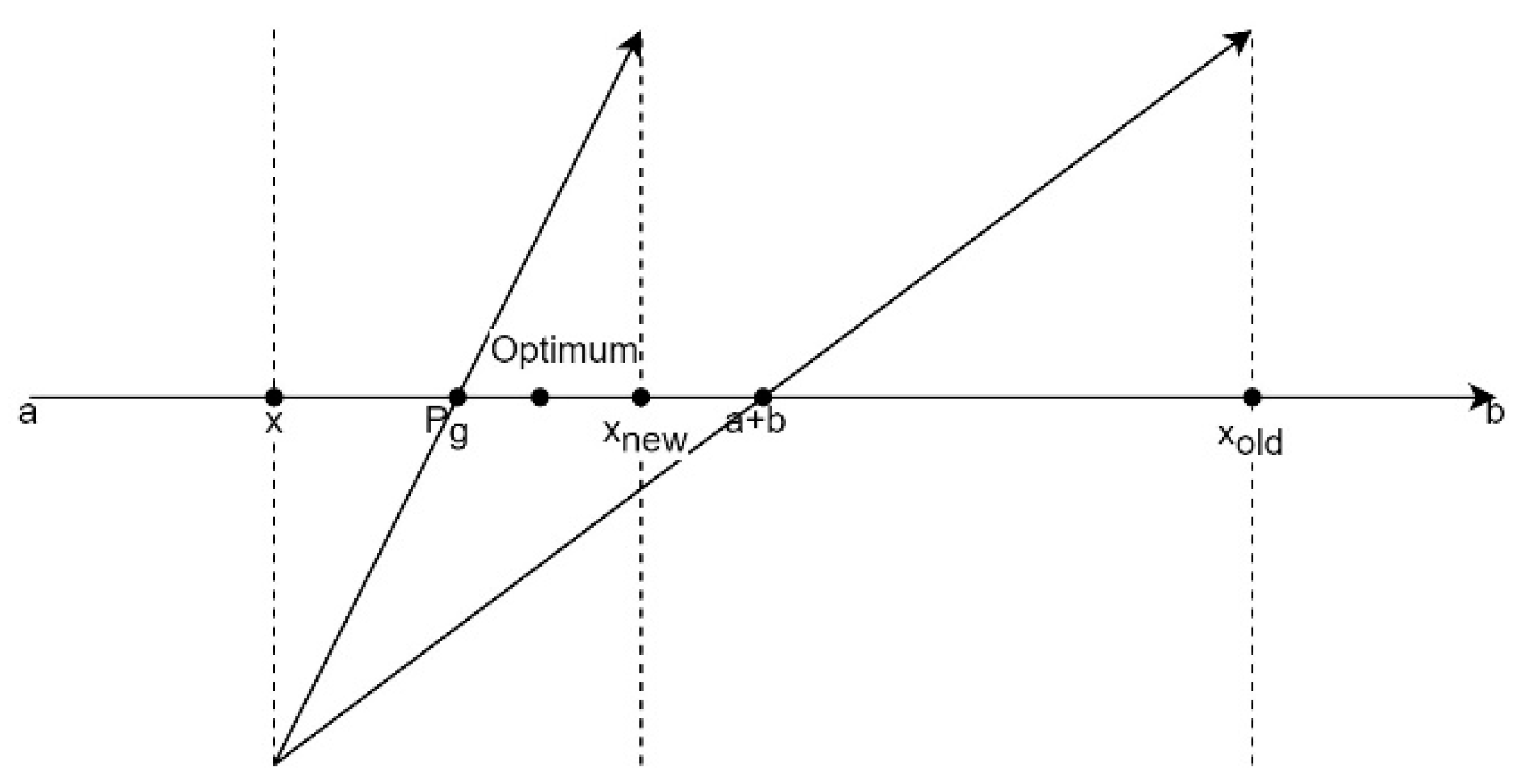
The opposition-based learning can produce a better solution for the searched solution, but these better solutions may be dispersed by the opposition-based learning at this point, which prevents the algorithm from finding the optimal solution in later iterations because most of beetles would gather at a point.
The opposition-based learning can be described as follows. New opposite solutions are obtained from current solutions by the way of symmetry at the middle point when the opposition-based learning formula is embodied in coordinates as Figure 1. In a search area, opposition-based learning is employed to make a new solution.
Next the novel opposition-based learning is put forward. Beetle individuals have the best location information (the optimal individual) in the BSO algorithm. Therefore, in the novel opposition-based learning process, the new solution is generated by a method similar to opposition-based learning. However, the difference between them is that the new solution in the novel opposition-based learning comes from the best location information (the optimal individual), not the middle point. In this method, when the current solution is far away from the optimal area, the new solution generated by this strategy can have a greater probability to be closer to the optimal solution to accelerate the convergence speed. Furthermore, because most beetles have already been near to the present optimal position in the later stages of iteration, the new solution obtained by continuing performing the novel opposition-based learning will not be far from the current optimal location.
The enhanced opposition-based learning formula can be defined as the following Equation (12) using the BSO algorithm.
x n e w = 2 P g x
where the term P g denotes the optimal solution of all current individuals, x denotes that the optimal solution of the current individual and x n e w denotes a newly generated optimal solution.
When the beetle swarm algorithm calculates a solution every time, the Equation (12) is employed to calculate a new solution to enhance population diversity.

3.2. The Adaptive Strategy

The displacement in the original BSO algorithm is weighted by the parameter λ , as can be seen from displacement formula (seen from Equation (7)). However, there is a key point here in that the value of λ is always a constant value, which results in a problem that beetles do not show greater group behavior that generated by randomly distribution in various positions in the searching space in the early stages of iteration. The group behavior allows them to swiftly gather to the optimal beetle, and most beetles will congregate near the optimal solution. At this moment, beetles should exhibit more individual behavior, so that instead of constantly traveling toward the current optimal beetle, they move according to individual behavior, which allows them to swiftly locate the optimal solution.
Therefore, based on the above idea, the formula for calculating λ can be defined as the following Equation (13):
λ = λ max ( λ max λ min ) T t
where t is the number of the current iteration, and T is the number of the maximum iteration.

3.3. Description of the Designed Algorithm

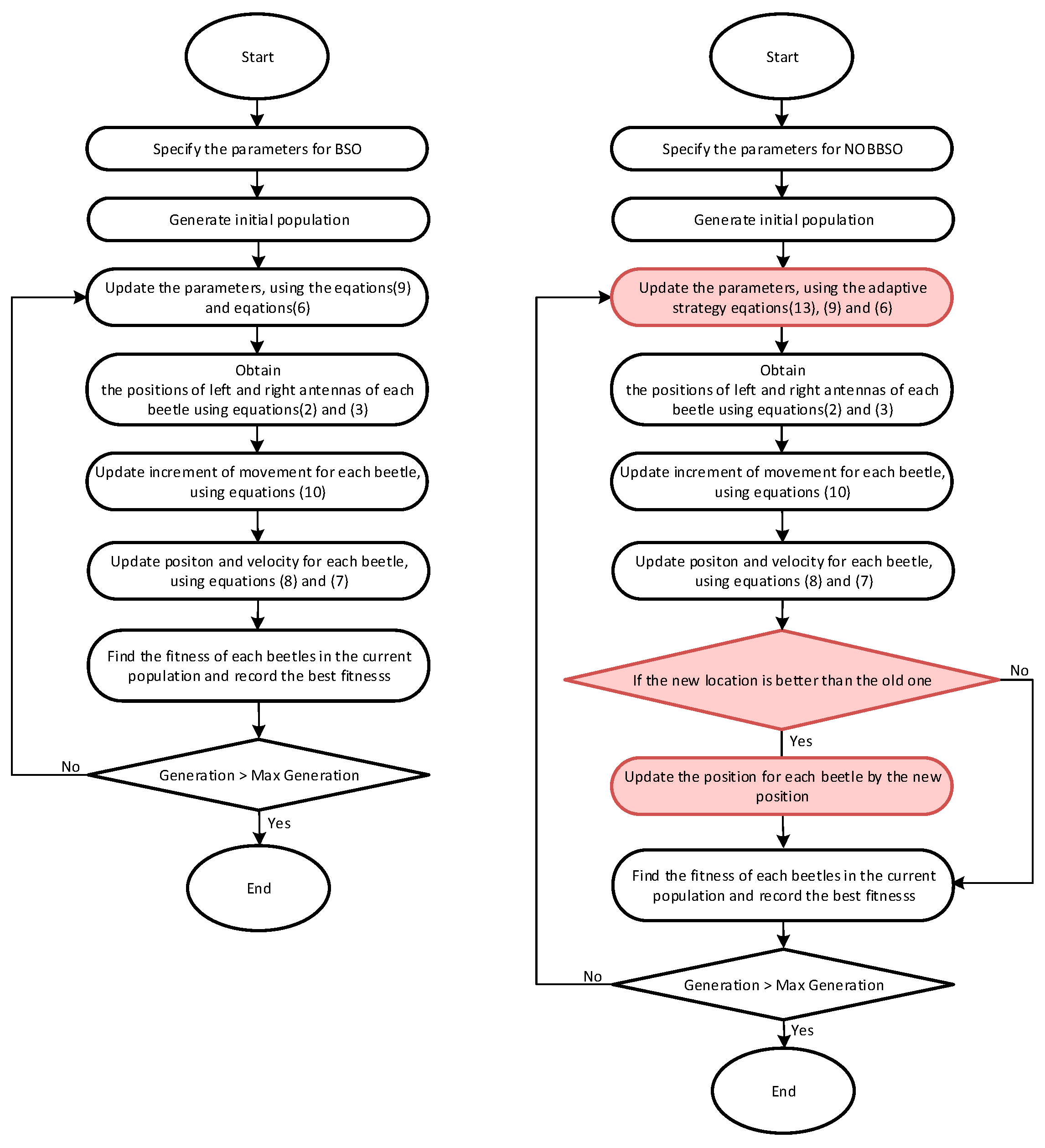
The performing process of the BSO algorithm is described as the following Algorithm 1:
Algorithm 1: BSO
S1: Initialize the beetle Xi, and population velocity v;
S2: Set step size, speed boundary, population size and maximum iteration and so on;
S3: The fitness of beetles is calculated;
S4: While (t <= T)
S5:  Equation (9) is used to calculate the weight w;
S6:  Update d using the Equation (6);
S7:  For every single beetle
S8:    Equations (2) and (3) are used to obtain the positions of left and right antennas of beetles, respectively;
S9:    Equation (10) is used to calculate the increment of the movement
S10:     Equation (8) is used to update beetle velocity V;
S11:     Use the Equation (7) to update the beetle position;
S12: End for
S13:     The fitness of each beetle is computed;
S14: Record and store the current location of the beetle;
S15 t = t + 1;
S16: End while
The performing process of the NOBBSO algorithm is described as the following Algorithm 2:
Algorithm 2: NOBBSO
S1: Initialize the beetle Xi, and population velocity v;
S2: Set step size, speed boundary, population size and maximum iteration and so on;
S3: The fitness of beetles is calculated;
S4:While (t <= T)
S5:  Equation (9) is used to calculate the weight w;
S6:  Update λ using the Equation (13);
S7:  Update d using the Equation (6);
S8:  For every single beetle
S9:     Equations (2) and (3) are used to obtain the positions of left and right antennas of beetles, respectively;
S10:    Equation (10) is used to calculate the increment of the movement
S11:    Equation (8) is used to update beetle velocity V;
S12:    Use the Equation (7) to update the beetle position;
S13:    Calculate the position of a new beetle using the Equation (12);
S14:    If the fitness of the new position is less than that of the beetle position
S15:    Update beetle position with a new beetle position;
S16:    End if
S17: End for
S18:  The fitness of each beetle is computed;
S19:  Record and store the current location of the beetle;
S20:  t = t + 1;
S21: End while
The performing process of the BSO and the NOBBSO algorithm is described as the following Figure 2:

4. The Experimental Verification

4.1. Related Parameter Settings and Test Functions

27 CEC2017 [20] benchmark functions (exclude f17, f20, f29) are used to test and compare the improved BSO algorithm with the original BSO algorithm to validate the performance of the improved BSO algorithm. The reason that these three functions are missing is that the original CEC2017 does not have a Python version, and here a third-party modified Python version of the CEC2017 is used (not include these three functions). Other two BSO algorithm are employed as competitors where BSO is the original beetle swarm algorithm and LBSO is the beetle swarm algorithm improved by Lévy flight. The initial population size of beetles is 50, and the dimension size of benchmark functions are set as 30. The number of iterations is 1000, and λ max and λ min are 1 and 0.4 respectively, and each function is repeated to run for 30 times. Related information of test problems is introduced briefly in Table 1.
It is worth noting that UF denotes the unimodal functions and SMF denotes the simple multimodal functions, and HF denotes the hybrid functions and CF denotes the composition functions.

4.2. The Experimental Method

4.2.1. Analysis of NOBBSO with Different Parameters

To test the performance of the algorithm in relation to the parameters, the following experiments investigate the effect of different parameters on the performance of the algorithm. In addition, the BSO and NOBBSO algorithms are compared on CEC2017 function 1 (Shifted and Rotated Bent Cigar). Population (Pop) sizes of 10, 20 and 30 are tested. Dimension (Dim) sizes of 10, 20 and 30 also are tested. The number of iterations is 1000.
The minimum values from Table 2 show that NOBBSO is easier to find the global optimal solution than the original BSO. However, it also shows some problems about NOBBSO. As the novel opposition-based learning generates a new solution, the solution is uncertain. As a result, the evaluation indicator (Std) of NOBBSO is worse than BSO.

4.2.2. Impact of Adaptive Strategies on Algorithms

In order to figure out the impact of adaptive strategy on NOBBSO, population and dimension parameters of both algorithms in this experiment are 30 while the parameter λ is set to different values as the following Table 3.
As can be seen from Table 3, the optimal solution with the adaptive strategy is superior to the algorithm without this strategy. Since λ is a constant value, the solution obtained with the increase of the parameter is more accurate. Therefore, the parameter is set adaptively to a changing value from the larger value to the smaller value, which makes the parameter the maximum value at the beginning of the iteration, and then decreases sequentially. Experiments show that adaptive strategy is very effective in the application of BSO.

4.2.3. Accuracy Results of Different Comparison Algorithms

Next, four evaluation indexes including Max, Min, Avg and Std which are the maximum value, minimum value, mean value and standard deviation respectively, and the test results are analyzed according to them, which are listed in Table 4.
According to the evaluating indicator (Min) results of the experiments in Table 4, the designed NOBBSO algorithm has 18 functions that are more accurate than the original BSO and LBSO while only 8 functions that are worse. Moreover, from the evaluation indicator (Avg) it can be seen that the NOBBSO algorithm outperforms the original BSO algorithm and LBSO algorithm over 19 out of 27 functions while only lose on 8 functions. Hence it can be observed that the convergence accuracy of the BSO algorithm in terms of average value can be significantly improved with the help of the improved opposition-based learning technique. Therefore, on the whole, the upgraded algorithms have a larger chance of discovering optimal solutions than the other comparison algorithms. Meanwhile it also shows that the improved opposition-based learning technique has better success in identifying optimal solutions.
Furthermore, the optimization ability of NOBBSO on unimodal functions and multimodal functions is stronger than the original algorithm, but the optimization ability on hybrid functions and composition functions is slightly superior to other algorithms in some functions.
Nonetheless, in the light of the evaluating indicator (Std) it can be seen that compared with the original BSO algorithm and LBSO algorithm, the NOBBSO algorithm only has 15 functions that are better than other two algorithms and 12 ones that are poorer than other ones. Meanwhile, from the evaluating indicator (Max), we can see that the NOBBSO algorithm only has 8 better outcomes while 19 poorer results. From these two evaluation indexes, as can be seen that the proposed NOBBSO algorithm shows the poor stability in dealing with the test problems.

4.2.4. Another Accuracy Results of Different Comparison Algorithms

To have a fair comparison, another statistical analysis experiments are performed. Unlike the previous experiments, the dimension size of benchmark functions is 10 and the number of iterations is 500 and other conditions are the same. These are listed in Table 5.
Compared with the original algorithm, NOBBSO obtains more accurate solutions on 10 functions. It is worth noting that there are nine functions that show that they have the same minimum value. The analysis shows that the optimization ability of the NOBBSO is stronger than the original algorithm. Moreover, the evaluation indicator (Avg) shows the optimal solution obtained by NOBBSO is generally more accurate than the original algorithm.

4.2.5. Convergence Analysis

Figure 3 represents the convergent curves of 27 CEC2017 benchmark functions that are performed on the above three BSO algorithms, where the scale of the y-axis is logarithmic.
The convergent curves of most functions show that NOBBSO obtains faster convergent speed than the classic BSO algorithm. Specifically, the analysis of the slopes of most functions clearly shows that the slope of NOBSO is better than the other algorithms, which suggests that NOBBSO has faster convergence speed than BSO, and also shows that it has the ability to search for the optimal solution more quickly.
However, unfortunately, for few functions such as f13, f15, f30, the convergence speed obtained by the NOBBSO algorithm is slower than the other algorithm, which means NOBBSO is attracted to locally optimal solutions, which results in its inability to find a better solution.

4.2.6. Friedman Test

A statistical mathematical analysis method, namely the Friedman test proposed by M. Friedman in 1973 [21], is used to reflect the differences among multiple samples. Average ranking is an index to evaluate the difference between samples in Friedman test. The smaller the value is, the greater the difference among samples is. For algorithms, the smaller the value is, it shows that there is a significant difference between the designed algorithm and the algorithm involved in the comparison within confidence level, that is, the performance of the designed algorithm is better than other algorithms because the average ranking is calculated by average values.
Table 6 lists the statistical results of Friedman test of three algorithms when the confidence level is 0.05.
We can see from the Table 6 that NOBBSO has obtained a minimum value that the average ranking represents, which demonstrates that the NOBBSO algorithm is different from other algorithms significantly.

5. Discussions

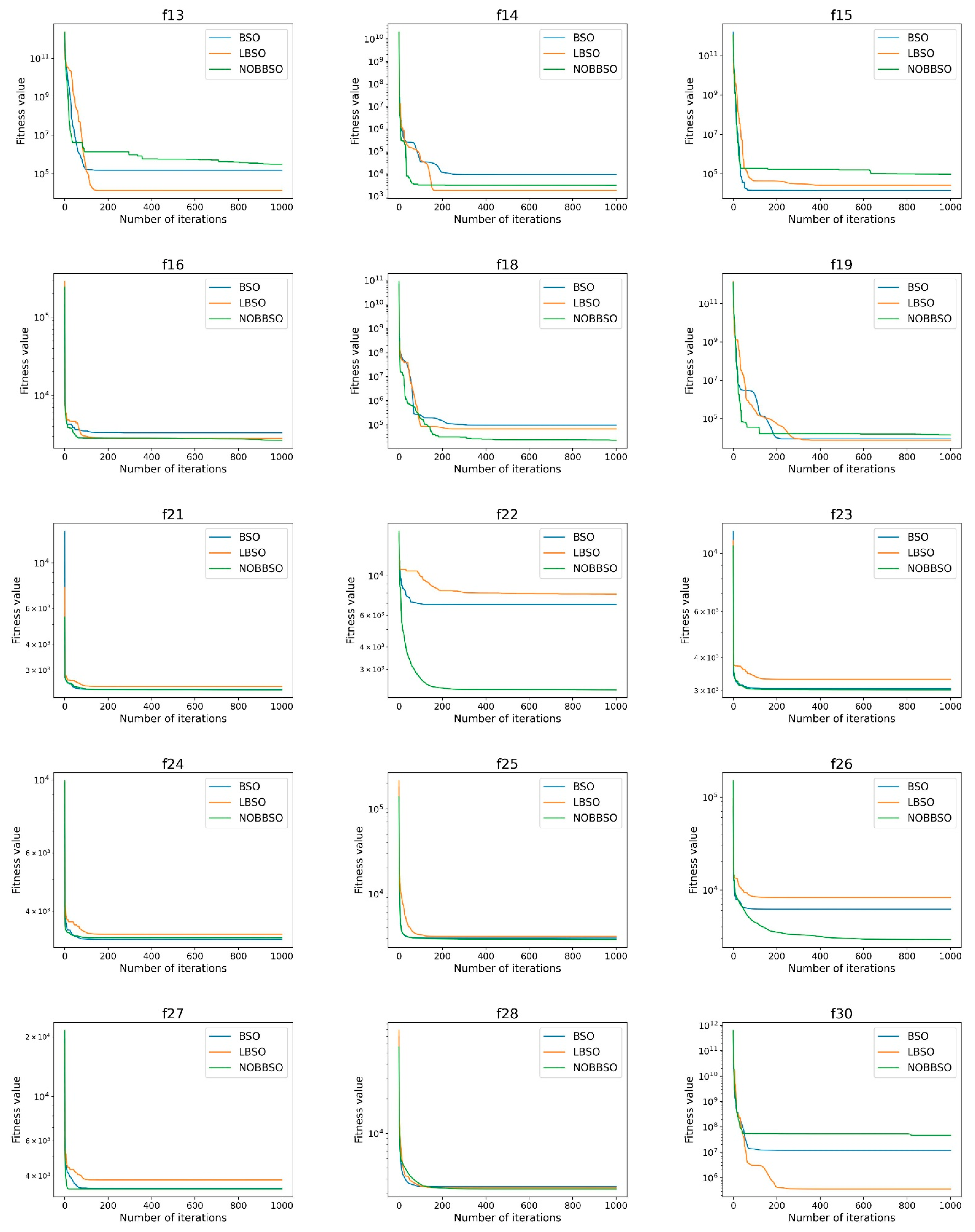
The numerical experiment results demonstrate that the NOBBSO algorithm has higher convergent speed and accuracy in comparison with other competitors.
However, NOBBSO is not a perfect algorithm either because its stability is not very good. For example, Table 3 shows that the λ parameter is continuously changed while the evaluation indicator (Std) does not change much. Therefore, the adaptive strategy is not the main reason for the impact on its stability and the fact reason is mainly from novel opposition-based learning. Because the new solution generated has also certain randomness, which can have an impact on its stability. Moreover, by analyzing Table 4 and Table 5, they show that NOBBSO is not much different from the original algorithm in obtaining the optimal solution in dealing with low dimension benchmark functions while NOBBSO is more accurate in obtaining the optimal solution in high dimensions, which demonstrates that the NOBBSO algorithm has advantages in dealing with higher dimensional problems.
From the worse results of few benchmark functions in Table 4 and Table 5, NOBBSO still has a certain probability to fall into the local optimal solution, but the probability of falling into a local optimum is actually less than the original algorithm on the whole. Hence it is still worth looking for better strategy or algorithms to improve it.

6. Conclusions

A novel algorithm called adaptive beetle swarm algorithm with novel opposition-based learning is proposed in this study. The algorithm is on the basis of the novel opposition-based learning and adaptive strategy to further enhance the optimization performance of the BSO algorithm. By testing 27 CEC2017 functions, the results show that the proposed NOBBSO algorithm has higher convergence accuracy and convergence speed.
In the future, NOBBSO can still be used in many places, because it is easy to converge and converges quickly. In engineering, there are many complex optimization problems that need to be solved well, but they are not quickly solved by traditional methods. Therefore, NOBBSO can be applied to solve them, which is also the future research work.

Author Contributions

Conceptualization, Q.W. and P.S.; methodology, Q.W. and P.S.; software, Q.W.; validation, Q.W., G.C. and P.S.; formal analysis, G.C. and P.S.; investigation, P.S.; resources, Q.W. and P.S.; data curation, Q.W. and P.S.; writing—original draft preparation, Q.W. and G.C; writing—review and editing, Q.W. and P.S.; visualization, Q.W.; supervision, P.S.; project administration, P.S.; funding acquisition, P.S. All authors have read and agreed to the published version of the manuscript.

Funding

This work is funded by the Technology Plan Projects of Jiangxi Provincial Education Department (No.GJJ200424).

Data Availability Statement

There is no data availability.

Conflicts of Interest

The authors declare that they have no known competing financial interests.

References

  1. Kennedy, J.; Eberhart, R. Particle Swarm Optimization. In Proceedings of the ICNN95-international Conference on Neural Networks, Perth, Australia, 27 November–1 December 1995. [Google Scholar]
  2. Karaboga, D.; Akay, B. A comparative study of Artificial Bee Colony algorithm. Appl. Math. Comput. 2009, 214, 108–132. [Google Scholar] [CrossRef]
  3. Parpinelli, R.S.; Lopes, H.S.; Freitas, A.A. Data mining with an ant colony optimization algorithm. Evol. Comput. IEEE Trans. 2002, 6, 321–332. [Google Scholar] [CrossRef] [Green Version]
  4. Wang, T.; Long, Y.; Qiang, L. Beetle Swarm Optimization Algorithm: Theory and Application. arXiv 2018, arXiv:1808.00206. [Google Scholar] [CrossRef]
  5. Wang, L.; Wu, Q.; Lin, F.; Li, S.; Chen, D. A New Trajectory-Planning Beetle Swarm Optimization Algorithm for Trajectory Planning of Robot Manipulators. IEEE Access 2019, 7, 154331–154345. [Google Scholar] [CrossRef]
  6. Hariharan, B.; Siva, R.; Kaliraj, S.; Prakash, P.N. ABSO: An energy-efficient multi-objective VM consolidation using adaptive beetle swarm optimization on cloud environment. J. Ambient. Intell. Humaniz. Comput. 2021, 1–13. [Google Scholar] [CrossRef]
  7. Mu, Y.; Li, B.; An, D.; Wei, Y. Three-Dimensional Route Planning Based on the Beetle Swarm Optimization Algorithm. IEEE Access 2019, 7, 117804–117813. [Google Scholar] [CrossRef]
  8. Singh, P.; Kaur, A.; Batth, R.S.; Kaur, S.; Gianini, G. Multi-disease big data analysis using beetle swarm optimization and an adaptive neuro-fuzzy inference system. Neural Comput. Appl. 2021, 33, 10403–10414. [Google Scholar] [CrossRef]
  9. Jiang, Y.; Wang, S.; Li, Y. Localizing and quantifying structural damage by means of a beetle swarm optimization algorithm. Adv. Struct. Eng. 2020, 24, 136943322095682. [Google Scholar] [CrossRef]
  10. Zhou, L.; Chen, K.; Dong, H.; Chi, S.; Chen, Z. An Improved beetle swarm optimization Algorithm for the Intelligent Navigation Control of Autonomous Sailing Robots. IEEE Access 2020, 9, 5296–5311. [Google Scholar] [CrossRef]
  11. Zhang, P.; Zhang, J.; Elsabbagh, A. Gait multi-objectives optimization of lower limb exoskeleton robot based on BSO-EOLLFF algorithm. Robotica 2022, 1–19. [Google Scholar] [CrossRef]
  12. Tizhoosh, H.R. Opposition-Based Learning: A New Scheme for Machine Intelligence. In Proceedings of the International Conference on International Conference on Computational Intelligence for Modelling, Control & Automation, Vienna, Austria, 28–30 November 2005; pp. 695–701. [Google Scholar]
  13. Wang, H.; Wu, Z.; Rahnamayan, S.; Liu, Y.; Ventresca, M. Enhancing particle swarm optimization using generalized opposition-based learning. Inf. Sci. 2011, 181, 4699–4714. [Google Scholar] [CrossRef]
  14. Shao, P.; Wu, Z.J.; Zhou, X.Y.; Deng, C.S. Improved Particle Swarm Optimization Algorithm Based on Opposite Learning of Refraction. Acta Electron. Sin. 2015, 25, 4117–4125. [Google Scholar]
  15. Zhou, X.Y.; Wu, Z.J.; Wang, H.; Li, K.S.; Zhang, H.Y. Elite Opposition-Based Particle Swarm Optimization. Acta Electron. Sin. 2013, 41, 1647–1652. [Google Scholar]
  16. Qian, Q.; Deng, Y.; Sun, H.; Pan, J.; Yin, J.; Feng, Y.; Fu, Y.; Li, Y. Enhanced beetle antennae search algorithm for complex and unbiased optimization. Soft Comput. 2022, 26, 10331–10369. [Google Scholar] [CrossRef] [PubMed]
  17. Zhao, J.; Lv, L.; Fan, T.; Wang, H.; Li, C.; Fu, P. Particle swarm optimization using elite opposition-based learning and application in wireless sensor network. Sens. Lett. 2014, 12, 404–408. [Google Scholar] [CrossRef]
  18. Mohammadzadeh, A.; Taghavifar, H. A robust fuzzy control approach for path-following control of autonomous vehicles. Soft Comput. 2020, 24, 3223–3235. [Google Scholar] [CrossRef]
  19. Jiang, X.; Li, S. BAS: Beetle Antennae Search Algorithm for Optimization Problems. arXiv 2017, arXiv:1710.10724. [Google Scholar] [CrossRef]
  20. Awad, N.H.; Ali, M.Z.; Suganthan, P.N.; Liang, J.J.; Qu, B.Y. Problem Definitions and Evaluation Criteria for the CEC 2017 Special Session and Competition on Single Objective Bound Constrained Real-Parameter Numerical Optimization; Nanyang Technological University Singapore: Singapore, 2016. [Google Scholar]
  21. Friedman, M. The use of ranks to avoid the assumption of normality implicit in the analysis of variance. J. Am. Stat. Assoc. 1937, 32, 675–701. [Google Scholar] [CrossRef]
Figure 1. The process of the novel opposition-based learning.
Electronics 11 03905 g001
Figure 2. Flowchart of BSO and NOBBSO (the left is the BSO flow chart and the right is the NOBBSO flow chart).
Electronics 11 03905 g002
Figure 3. The analysis diagram of convergence.
Electronics 11 03905 g003aElectronics 11 03905 g003b
Table 1. Test functions.
TypesNo.FunctionsOptimal
UFf1Shifted and Rotated Bent Cigar100
f2Shifted and Rotated Sum of Different Power200
SMFf3Shifted and Rotated Zakharov300
f4Shifted and Rotated Rosenbrock400
f5Shifted and Rotated Rastrigin500
f6Shifted and Rotated Expanded Scaffer’s F6600
f7Shifted and Rotated Lunacek Bi_Rastrigin700
f8Shifted and Rotated Non-Continuous Rastrigin800
f9Shifted and Rotated Lévy900
f10Shifted and Rotated Schwefel1000
HFf11Hybrid Function 1 (N = 3)1100
f12Hybrid Function 2 (N = 3)1200
f13Hybrid Function 3 (N = 3)1300
f14Hybrid Function 4 (N = 4)1400
f15Hybrid Function 5 (N = 4)1500
f16Hybrid Function 6 (N = 4)1600
f18Hybrid Function 6 (N = 5)1800
f19Hybrid Function 6 (N = 5)1900
CFf21Composition Function 1 (N = 3)2100
f22Composition Function 2 (N = 3)2200
f23Composition Function 3 (N = 4)2300
f24Composition Function 4 (N = 4)2400
f25Composition Function 5 (N = 5)2500
f26Composition Function 6 (N = 5)2600
f27Composition Function 7 (N = 6)2700
f28Composition Function 8 (N = 6)2800
f30Composition Function 10 (N = 3)3000
Search Range: [−100, 100]S
Table 2. The analysis of parameters.
ParametersAlgorithmsMinMaxAvgStd
Pop = 10BSO2.63 × 1071.89 × 10126.32 × 1094.51 × 1010
Dim = 10NOBBSO1.02 × 1051.89 × 10127.47 × 1094.81 × 1010
Pop = 10BSO6.08 × 1092.85 × 10127.76 × 10108.93 × 1010
Dim = 20NOBBSO1.66 × 1072.45 × 10123.14 × 10108.86 × 1010
Pop = 10BSO1.45 × 10114.29 × 10122.78 × 10111.59 × 1011
Dim = 30NOBBSO4.00 × 1094.17 × 10121.41 × 10111.72 × 1011
Pop = 20BSO2.67 × 1042.00 × 10123.07 × 1094.82 × 1010
Dim = 10NOBBSO8.33 × 1041.80 × 10123.20 × 1094.81 × 1010
Pop = 20BSO1.32 × 1092.89 × 10122.47 × 10108.23 × 1010
Dim = 20NOBBSO1.76 × 1062.79 × 10121.20 × 10108.42 × 1010
Pop = 20BSO2.65 × 10105.16 × 10129.20 × 10101.51 × 1011
Dim = 30NOBBSO3.42 × 1074.30 × 10123.47 × 10101.50 × 1011
Pop = 30BSO1.16 × 1022.20 × 10122.69 × 1095.12 × 1010
Dim = 10NOBBSO2.02 × 1041.93 × 10122.47 × 1094.87 × 1010
Pop = 30BSO3.44 × 1082.66 × 10121.26 × 10108.15 × 1010
Dim = 20NOBBSO1.02 × 1062.94 × 10129.68 × 1098.31 × 1010
Pop = 30BSO8.18 × 1094.71 × 10125.36 × 10101.45 × 1011
Dim = 30NOBBSO7.86 × 1064.82 × 10122.65 × 10101.50 × 1011
Statistical results7/96/97/94/9
Table 3. The analysis of adaptive strategy.
λMinMaxAvgStd
0.16.56 × 10105.27 × 10121.24 × 10111.38 × 1011
0.252.41 × 10104.76 × 10127.26 × 10101.40 × 1011
0.51.00 × 1074.46 × 10121.76 × 10101.45 × 1011
0.755.20 × 1064.80 × 10121.77 × 10101.51 × 1011
0.94.46 × 1064.45 × 10121.89 × 10101.50 × 1011
Adaptive (Equation (13))3.73 × 1065.00 × 10121.91 × 10101.49 × 1011
Table 4. Accurate results of three algorithms when D is 30.
FunctionsAlgorithmsMinMaxAvgStd
f1BSO2.83 × 1094.42 × 10122.80 × 10101.44 × 1011
LBSO1.89 × 1074.65 × 10122.20 × 10101.62 × 1011
NOBBSO1.62 × 1064.60 × 10121.90 × 10101.45 × 1011
f2BSO7.73 × 10201.89 × 10731.61 × 10691.28 × 1071
LBSO8.43 × 10133.41 × 10733.53 × 10692.77 × 1071
NOBBSO3.32 × 1077.87 × 10737.32 × 10696.03 × 1071
f3BSO1.81 × 1042.49 × 10169.55 × 10123.58 × 1014
LBSO1.19 × 1032.56 × 10161.11 × 10134.13 × 1014
NOBBSO3.11 × 1021.94 × 10168.71 × 10123.17 × 1014
f4BSO5.47 × 1025.38 × 1051.41 × 1031.36 × 104
LBSO4.69 × 1026.41 × 1051.46 × 1031.42 × 104
NOBBSO4.59 × 1025.60 × 1051.22 × 1031.29 × 104
f5BSO6.45 × 1022.28 × 1037.08 × 1026.42 × 101
LBSO6.36 × 1022.27 × 1037.02 × 1026.98 × 101
NOBBSO6.13 × 1022.20 × 1036.86 × 1026.96 × 101
f6BSO6.47 × 1021.03 × 1036.68 × 1021.61 × 101
LBSO6.46 × 1021.02 × 1036.72 × 1021.59 × 101
NOBBSO6.39 × 1021.01 × 1036.60 × 1021.70 × 101
f7BSO1.01 × 1037.59 × 1031.21 × 1032.36 × 102
LBSO9.26 × 1027.34 × 1031.05 × 1032.47 × 102
NOBBSO9.10 × 1028.07 × 1031.08 × 1032.29 × 102
f8BSO8.80 × 1022.40 × 1039.50 × 1026.44 × 101
LBSO8.76 × 1022.18 × 1039.51 × 1026.34 × 101
NOBBSO8.83 × 1022.29 × 1039.45 × 1025.95 × 101
f9BSO2.83 × 1031.89 × 1055.08 × 1035.02 × 103
LBSO2.77 × 1031.96 × 1055.12 × 1035.30 × 103
NOBBSO2.57 × 1031.99 × 1055.00 × 1035.14 × 103
f10BSO4.70 × 1031.71 × 1046.93 × 1031.33 × 103
LBSO4.00 × 1031.67 × 1045.81 × 1031.13 × 103
NOBBSO4.29 × 1031.69 × 1046.23 × 1031.15 × 103
f11BSO1.31 × 1036.65 × 10113.11 × 1081.09 × 1010
LBSO1.16 × 1036.61 × 10113.29 × 1081.14 × 1010
NOBBSO1.19 × 1039.15 × 10114.27 × 1081.52 × 1010
f12BSO2.96 × 1071.34 × 10122.89 × 1093.67 × 1010
LBSO1.67 × 1061.34 × 10124.00 × 1094.09 × 1010
NOBBSO1.51 × 1061.43 × 10122.14 × 1093.70 × 1010
f13BSO9.80 × 1032.66 × 10123.36 × 1097.22 × 1010
LBSO1.37 × 1042.86 × 10124.97 × 1097.27 × 1010
NOBBSO7.43 × 1042.68 × 10123.04 × 1096.97 × 1010
f14BSO1.76 × 1033.72 × 10102.48 × 1078.00 × 108
LBSO1.67 × 1033.75 × 10102.54 × 1078.11 × 108
NOBBSO1.96 × 1033.89 × 10102.37 × 1077.71 × 108
f15BSO5.74 × 1031.56 × 10121.21 × 1093.40 × 1010
LBSO2.00 × 1031.50 × 10121.54 × 1093.59 × 1010
NOBBSO1.04 × 1041.54 × 10121.29 × 1093.54 × 1010
f16BSO2.68 × 1035.39 × 1053.60 × 1039.43 × 103
LBSO2.16 × 1034.69 × 1053.42 × 1031.00 × 104
NOBBSO2.09 × 1035.45 × 1053.22 × 1031.02 × 104
f18BSO4.30 × 1049.96 × 10107.47 × 1072.32 × 109
LBSO1.56 × 1041.12 × 10118.17 × 1072.50 × 109
NOBBSO3.66 × 1041.22 × 10118.35 × 1072.61 × 109
f19BSO8.49 × 1031.85 × 10121.40 × 1093.81 × 1010
LBSO2.11 × 1031.63 × 10121.57 × 1093.71 × 1010
NOBBSO7.15 × 1031.64 × 10121.26 × 1093.54 × 1010
f21BSO2.41 × 1031.60 × 1042.49 × 1031.97 × 102
LBSO2.44 × 1031.37 × 1042.53 × 1031.90 × 102
NOBBSO2.38 × 1031.11 × 1042.47 × 1031.62 × 102
f22BSO2.55 × 1031.99 × 1045.92 × 1032.37 × 103
LBSO2.32 × 1031.83 × 1045.20 × 1032.58 × 103
NOBBSO2.31 × 1031.92 × 1045.49 × 1032.80 × 103
f23BSO2.96 × 1031.28 × 1043.13 × 1032.66 × 102
LBSO3.11 × 1031.27 × 1043.34 × 1032.89 × 102
NOBBSO2.81 × 1031.36 × 1043.04 × 1032.79 × 102
f24BSO3.07 × 1031.15 × 1043.35 × 1032.40 × 102
LBSO3.13 × 1031.10 × 1043.38 × 1032.56 × 102
NOBBSO3.03 × 1031.16 × 1043.19 × 1032.46 × 102
f25BSO2.96 × 1033.22 × 1053.30 × 1036.07 × 103
LBSO2.90 × 1032.88 × 1053.24 × 1036.08 × 103
NOBBSO2.88 × 1032.45 × 1053.19 × 1035.84 × 103
f26BSO3.53 × 1031.86 × 1057.51 × 1033.45 × 103
LBSO2.87 × 1031.68 × 1057.08 × 1033.87 × 103
NOBBSO2.83 × 1031.99 × 1057.23 × 1034.04 × 103
f27BSO3.41 × 1034.24 × 1043.70 × 1036.96 × 102
LBSO3.36 × 1032.67 × 1043.78 × 1036.37 × 102
NOBBSO3.24 × 1033.04 × 1043.47 × 1036.25 × 102
f28BSO3.32 × 1031.43 × 1053.64 × 1032.82 × 103
LBSO3.21 × 1031.60 × 1053.49 × 1032.78 × 103
NOBBSO3.18 × 1031.38 × 1053.47 × 1032.67 × 103
f30BSO5.98 × 1058.30 × 10117.19 × 1081.91 × 1010
LBSO3.27 × 1048.68 × 10119.47 × 1082.00 × 1010
NOBBSO1.29 × 1057.64 × 10116.86 × 1081.88 × 1010
Statistical results18/278/2719/2715/27
Table 5. Accurate results of two algorithms when D is 10.
FunctionsAlgorithmsMinMaxAvgStd
f1BSO5.63 × 1021.96 × 10125.26 × 1097.50 × 1010
NOBBSO2.12 × 1041.92 × 10124.70 × 1097.34 × 1010
f2BSO2.63 × 1036.80 × 10228.44 × 10192.03 × 1021
NOBBSO2.00 × 1026.62 × 10226.04 × 10191.57 × 1021
f3BSO3.10 × 1029.59 × 10121.09 × 10102.69 × 1011
NOBBSO3.00 × 1021.93 × 10131.90 × 10104.73 × 1011
f4BSO4.00 × 1021.32 × 1056.29 × 1024.52 × 103
NOBBSO4.00 × 1021.75 × 1056.47 × 1025.09 × 103
f5BSO5.07 × 1021.28 × 1035.31 × 1023.40 × 101
NOBBSO5.07 × 1021.25 × 1035.26 × 1023.52 × 101
f6BSO6.16 × 1021.15 × 1036.37 × 1022.16 × 101
NOBBSO6.05 × 1021.11 × 1036.19 × 1022.21 × 101
f7BSO7.23 × 1022.73 × 1037.63 × 1028.88 × 101
NOBBSO7.25 × 1022.83 × 1037.42 × 1028.75 × 101
f8BSO8.09 × 1021.29 × 1038.23 × 1022.41 × 101
NOBBSO8.07 × 1021.30 × 1038.21 × 1022.34 × 101
f9BSO9.42 × 1028.74 × 1041.23 × 1032.68 × 103
NOBBSO9.04 × 1026.62 × 1041.10 × 1032.36 × 103
f10BSO1.53 × 1037.04 × 1032.22 × 1034.73 × 102
NOBBSO1.39 × 1037.03 × 1032.14 × 1035.41 × 102
f11BSO1.11 × 1031.54 × 10102.45 × 1075.56 × 108
NOBBSO1.11 × 1031.44 × 10102.29 × 1075.23 × 108
f12BSO5.71 × 1034.81 × 10117.93 × 1081.68 × 1010
NOBBSO3.78 × 1033.95 × 10117.18 × 1081.51 × 1010
f13BSO2.33 × 1033.55 × 10116.01 × 1081.33 × 1010
NOBBSO2.48 × 1033.49 × 10116.07 × 1081.35 × 1010
f14BSO1.49 × 1032.88 × 10104.48 × 1071.01 × 109
NOBBSO1.49 × 1032.89 × 10104.89 × 1071.10 × 109
f15BSO1.58 × 1035.40 × 10118.96 × 1082.03 × 1010
NOBBSO1.75 × 1034.98 × 10118.58 × 1081.93 × 1010
f16BSO1.62 × 1031.74 × 1052.08 × 1035.27 × 103
NOBBSO1.60 × 1031.96 × 1052.04 × 1036.49 × 103
f18BSO2.05 × 1031.26 × 10112.08 × 1084.64 × 109
NOBBSO2.05 × 1031.17 × 10111.95 × 1084.37 × 109
f19BSO1.93 × 1031.08 × 10121.77 × 1093.99 × 1010
NOBBSO1.99 × 1039.87 × 10111.69 × 1093.82 × 1010
f21BSO2.20 × 1031.20 × 1042.24 × 1032.75 × 102
NOBBSO2.20 × 1031.21 × 1042.30 × 1032.55 × 102
f22BSO2.30 × 1038.02 × 1032.35 × 1032.81 × 102
NOBBSO2.30 × 1039.12 × 1032.33 × 1032.78 × 102
f23BSO2.62 × 1037.25 × 1032.68 × 1031.85 × 102
NOBBSO2.61 × 1037.08 × 1032.64 × 1031.73 × 102
f24BSO2.50 × 1038.79 × 1032.75 × 1032.23 × 102
NOBBSO2.50 × 1037.29 × 1032.71 × 1032.06 × 102
f25BSO2.90 × 1033.88 × 1043.01 × 1031.37 × 103
NOBBSO2.90 × 1034.33 × 1042.99 × 1031.39 × 103
f26BSO2.80 × 1032.93 × 1043.23 × 1038.67 × 102
NOBBSO2.90 × 1033.03 × 1043.04 × 1038.87 × 102
f27BSO3.11 × 1032.50 × 1043.18 × 1037.47 × 102
NOBBSO3.10 × 1032.76 × 1043.16 × 1038.88 × 102
f28BSO3.11 × 1032.68 × 1043.38 × 1038.06 × 102
NOBBSO3.17 × 1031.69 × 1043.38 × 1034.77 × 102
f30BSO4.22 × 1032.50 × 10113.51 × 1087.96 × 109
NOBBSO1.24 × 1042.34 × 10113.43 × 1087.88 × 109
Statistical results10/2716/2721/2716/27
Table 6. Statistical results.
AlgorithmsAverage Ranking
BSO2.52
LBSO2.41
NOBBSO1.42
Publisher’s Note: MDPI stays neutral with regard to jurisdictional claims in published maps and institutional affiliations.

