Robust Data-Driven Design for Fault Diagnosis of Industrial Drives

Abstract

Due to the presence of actuator disturbances and sensor noise, increased false alarm rate and decreased fault detection rate in fault diagnosis systems have become major concerns. Various performance indexes are proposed to deal with such problems with certain limitations. This paper proposes a robust performance-index based fault diagnosis methodology using input–output data. That data is used to construct robust parity space using the subspace identification method and proposed performance index. Generated residual shows enhanced sensitivity towards faults and robustness against unknown disturbances simultaneously. The threshold for residual is designed using the Gaussian likelihood ratio, and the wavelet transformation is used for post-processing. The proposed performance index is further used to develop a fault isolation procedure. To specify the location of the fault, a modified fault isolation scheme based on perfect unknown input decoupling is proposed that makes actuator and sensor residuals robust against disturbances and noise. The proposed detection and isolation scheme is implemented on the induction motor in the experimental setup. The results have shown the percentage fault detection of 98.88%, which is superior among recent research.

1. Introduction

The early and accurate detection of abnormal events is crucial for today’s safety-critical systems with their continuously increasing complexity. Model based fault diagnosis has enjoyed considerable attention during the last three decades and provides a rich literature of techniques considering practical solutions for fault diagnosis [1,2,3,4,5,6,7]. High-fidelity modeling requirements for model based fault diagnosis make it difficult and sometimes infeasible to implement for the complex system. Noteworthy examples from these complicated systems are networked control systems, internet of things [8], and different chemical industry processes [9]. A sufficient amount of data is available for the majority of such systems. This data contain information about the system, disturbances and noise, fault, and so on. To deal with such systems, various data-driven methods are being used with effective implementation.

These methods are broadly classified into two classes [10]: (1) data-driven methodologies [11,12]; (2) model-data based hybrid approaches [13,14,15]. Among various pure data based methods, machine learning [16], deep learning [17,18], and multivariate techniques including principal component analysis [19,20,21] and partial least square methods [22,23,24] are widely used with promising results. A model-data based hybrid approach usually considers the development of FDI schemes that consists of an intersection between model based and data-driven techniques [13]. Subspace identification method (SIM) emerged as one of the major techniques in this domain for the last two decades [25,26,27,28]. The key concept behind the Subspace identification method (SIM) approach is to identify the parity space for the construction of observer based fault detection and isolation (FDI) scheme [26] or parity based FDI residual generators [27] using input–output data. The effect of external factors such as noise and disturbances from recorded data are eliminated by introducing instrument variables. Finding orthogonal projection of an extended observability matrix enables constructing residuals based on a parity vector, which is made possible by using the singular value decomposition (SVD) on covariance matrices of recorded data [29]. Since the Subspace identification method (SIM) is developed to estimate the dynamic model of the underlying system, it is worth mentioning that it also solves the problem of dealing with stationary as well as dynamical systems, compared to multivariate analysis (MVA) techniques which are operated on stationary processes. Although several MVA techniques have been developed to deal with dynamic issues, these are not suitable for stationary processes [30].

Subspace identification has been applied to many practical systems including the Tennessee Eastman process [26,31], vehicle lateral dynamic system [27], coupled liquid tank system [32], wind turbine benchmark [33,34,35], and three phase induction motor [36,37]. Since induction motors play a vital role in the process industry for converting electromechanical energy and are the most widely used devices [38], our study would be directed toward implementing data-driven techniques on an induction motor. Due to the critical operation of induction motors in industries such as power generation, petroleum [39], aerospace [40], and the medical industry, it is required to monitor the reliability and running conditions to avoid any disastrous failures. Now, operators have started using rapid fault detection along with the usually planned maintenance, which could reduce the failure rate, increase the plant uptime, and reduce operational and maintenance costs.

The induction motor and its drive system could be subjected to different types of faults. Some of them could be [41,42]:

• Stator fault that includes short and open circuiting of the stator winding;
• Rotor faults dealing with end-ring cracking in the case of squirrel cage motor and short or open circuiting of the rotor winding;
• Power supply failure due to power electronics damage of the driving system;
• Mechanical fault including bearing damage, eccentricity misalignment, and a bent shaft.

Since induction motors are considered symmetrical machines, any fault could modify their operational behavior by changing symmetrical properties.

Machine learning and model-based methodologies have also been applied to induction motor for fault detection and isolation purposes. Convolutional neural network (CNN) based fault diagnosis and classification was carried out by Maciej Skowron in [43]. During the fault detection process, a neural network also acts as a classification system which also identifies degree of damage to the induction motor. Choosing a right structure of CNN for fault detection and isolation (FDI) system plays a vital role in methodology, as a minor change could lead to a huge increase in false alarm rate (FAR). Data based and model based techniques have their own advantages and disadvantages in different system states. Unknown faults can be detected and identified efficiently by model based methods while data based methodologies mostly analyse the input–output signal of the induction motor giving low weight to system dynamics [44]. Hybrid approaches, which are a combination of system model based FDI schemes and pure data based methodologies, have shown great ability to detect fault and analyse fault with unbalanced conditions [45].

Parity equation based methods provide less online computational complexity which leads to early detection of faults [46]. In our FDI scheme, parity space is identified using a subspace identification method which is further used for residual generation. For the subspace method, it is challenging to find an optimal parity vector that makes generated residuals more sensitive towards fault and less sensitive towards external factors (e.g., noise and disturbances) simultaneously. To face such challenges, various performance indexes are proposed [26,27,32,37] for the computation of optimal parity vector. In [27], a proposed index considers the sensitivity for actuator and sensor faults but does not consider the effect of unknown inputs. Similarly, Ref. [32] proposed a performance index that considers the effect of actuator disturbance and actuator fault sensitivity in generated residual. Till then, enhancement of sensitivity towards sensor faults and sensor noise was discussed. However, Ref. [37] proposed a methodology to optimize the parity vector for sensor fault and noise at the expense of actuator fault and disturbance.

In this paper, we have developed the subspace-based data-driven fault diagnosis scheme for dynamical systems based on the proposed performance index, which makes the residual sensitive towards actuator and sensor faults simultaneously while suppressing the effect of unknown inputs such as actuator disturbances and sensor noise. Furthermore, to determine the location of the faulty component, an isolation algorithm based on perfect unknown input decoupling is proposed with an improved performance index for an optimized parity vector.

The rest of the paper is organized as follows: Section 2 includes dynamic consideration of induction motor used for online implementation. Section 3 states the fundamentals of the subspace identification method and mathematical derivations. Proposed fault detection and isolation algorithms are also stated in Section 3 and Section 4, respectively. Section 5 is related to the post-processing of residuals, which include wavelet transformation and Gaussian Likelihood Ration test. Practical implementation of developed schemes is then implemented on an induction motor as described in Section 6. Section 7 concludes with a summary of the work.

2. Induction Motor Dynamics

The induction motor is operated by applying AC voltage to the stator, which produces the AC current in the rotor circuit. Since there is no electrical connection between the rotor and stator of the induction motor, it makes the motor almost maintenance-free and more efficient due to no power loss in the commutators. Squirrel cage induction motors are the most commonly used motor varying from a few to hundreds of horsepower. The rotor rotates when it is subjected to varying magnetic fields, and the speed of the rotor depends upon the frequency $\left(f_e\right)$ of applied voltage and stator poles $\left(p\right)$ of the motor as described in Equation (1):

$$n_{sync}=\frac{120f_e}{p}$$

(1)

A mathematical model of the motor could be constructed by considering the equivalent model of a signal phase induction motor. The nominal parameters of induction motor under consideration are given in

Table 1. Induction Motor Nominal Parameters (SE2672-3G).

Name	Symbol	Value
Number of poles	$P_n$	2
Inductance of Rotor	$L_{rot}$	0.1164
Resistance of Rotor	$R_{rot}$	3.5735
Inductance of Stator	$L_{sat}$	0.1164
Resistance of Stator	$R_{sat}$	0.7941
Leakage factor	$\sigma$	0.092896
Mutual inductance	$L_{s,r}$	0.1109

. A 5th order state-space model of the induction motor is constructed based on the stator-fixed frame reference:

$$\left\{\begin{array}{c}\dot{{\eta }_1}=c_4{\eta }_1-P_n{\eta }_5{\eta }_2+c_5{\eta }_3\hfill \\ \dot{{\eta }_2}=P_n{\eta }_5{\eta }_1+c_4{\eta }_2+c_5{\eta }_4\hfill \\ \dot{{\eta }_3}=c_6{\eta }_1+c_7{\eta }_5{\eta }_2-\gamma {\eta }_3+c_8{u}_1\hfill \\ \dot{{\eta }_4}=-c_7{\eta }_5{\eta }_1+c_6{\eta }_2-\gamma {\eta }_4+c_8{u}_2\hfill \\ \dot{{\eta }_5}=c_1{\eta }_1{\eta }_4+c_2{\eta }_5+c_3{\tau }_L-c_1{\eta }_2{\eta }_3\hfill \\ y=[{\eta }_3,{\eta }_4]\hfill \end{array}\right.$$

(2)

Here, the state vector is representing the d-q axis fluxes and current along with the speed of rotor, such that $\eta ={\left[{\eta }_1{\eta }_2{\eta }_3{\eta }_4{\eta }_5\right]}^T={\left[{\varphi }_d{\varphi }_q{i}_d{i}_q\omega \right]}^T$. Since motor is being activated by the three phase voltage, the acting actuator input would be these supply voltages.

Constants used in the model (2) are defined as

$$\begin{array}{cccccc}\hfill c_1& =\frac{P_n{L}_{s,r}}{D_m{L}_{rot}},\hfill & \hfill c_2& =-\frac{R_m}{D_m},\hfill & \hfill c_3& =-\frac{1}{D_m}\hfill \\ \hfill c_4& =-\frac{1}{T_r},\hfill & \hfill c_5& =\frac{L_{s,r}}{T_r},\hfill & \hfill c_6& =\frac{L_{s,r}}{T_r\sigma L_{sat}{L}_{rot}}\hfill \\ \hfill c_7& =\frac{P_n{L}_{s,r}}{\sigma L_{sat}{L}_{rot}},\hfill & \hfill c_8& =\frac{1}{\sigma L_{sat}}\hfill \end{array}$$

further,

$$\begin{array}{cccc}\hfill \gamma & =\frac{R_{sat}}{L_{sat}\sigma }+\frac{L_{s,r}^2}{\sigma L_{sat}{L}_{rot}{T}_{rot}},\hfill & \hfill \sigma & =1-\frac{L_{s,r}^2}{L_{sat}{L}_{rot}}\hfill \\ \hfill T_r& =\frac{L_{rot}}{R_{rot}}\hfill \end{array}$$

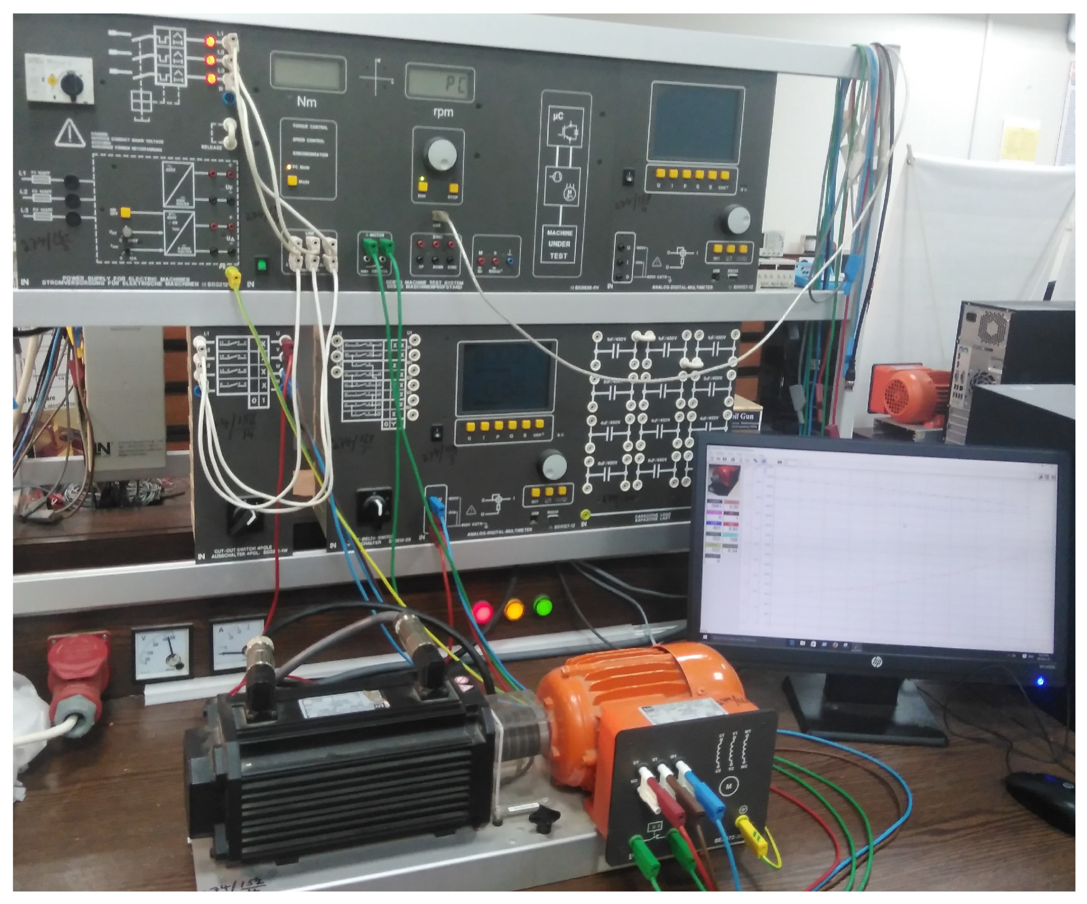
Thus, the dynamic model for an induction motor (SE2672-3G) as shown in Figure 1 could be found using values given in Table 1. Besides nominal parameters, the nominal operating conditions of motor are stated in

Table 2. Nominal operating conditions (SE2672-3G).

Parameter	Value
Nominal Voltage $\Delta$/Y	400/690 V
Nominal Current $\Delta$/Y	1.0/0.6 A
Nominal Power	370 W
Power Factor	0.83
Frequency	50 Hz
Nominal Speed	2800 rpm

.

3. Fault Diagnosis Scheme

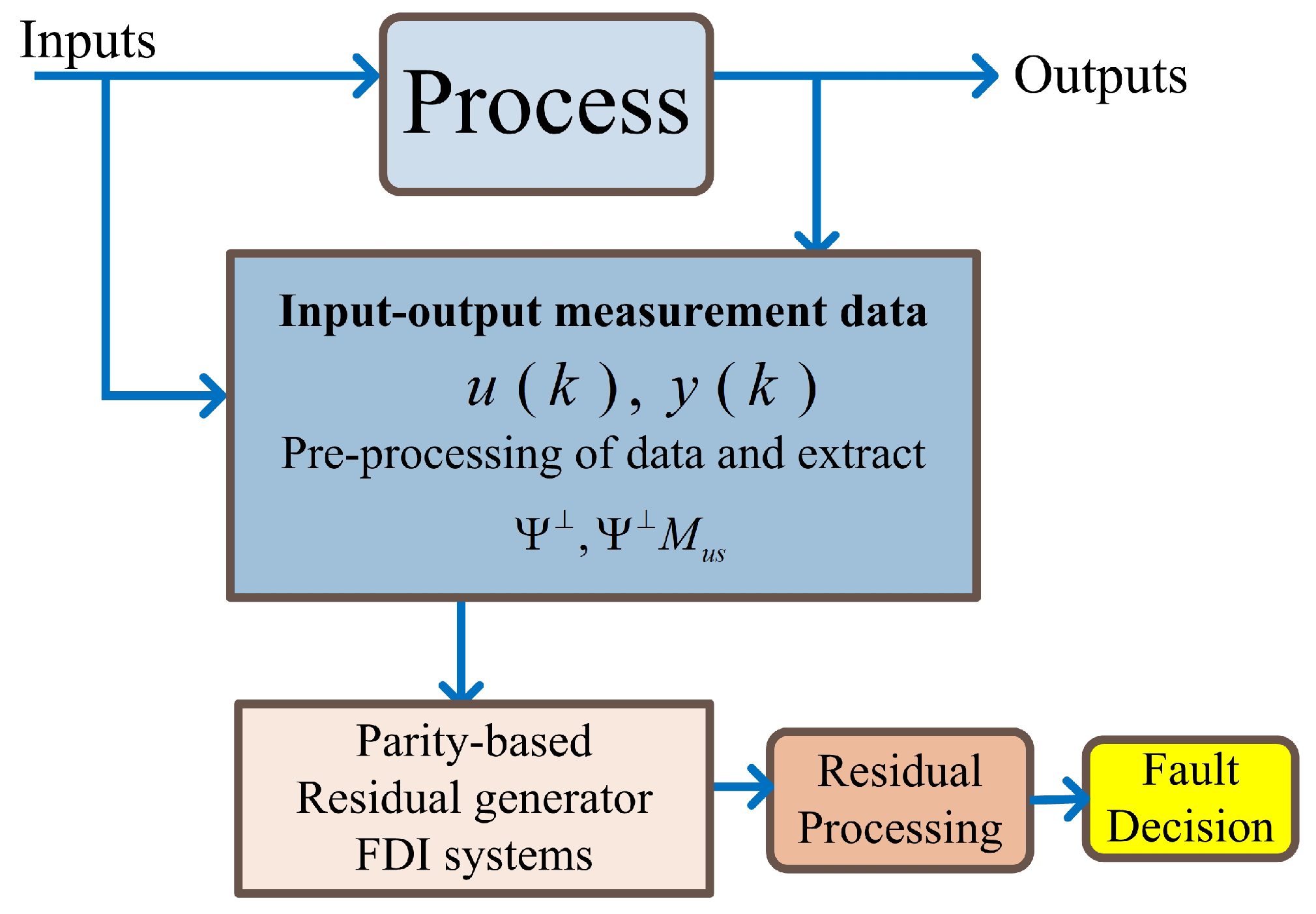
Parity vector-based residual generation is one of the famous fault diagnosis schemes used in both model-based and data-driven FDI systems [47]. The parity vector scheme allows us to use techniques developed in model-based FDI literature for data-driven systems. In order to obtain the advantage of the availability of input–output data samples of the process and avoid complexity issues to obtain a system model, the subspace identification mechanism is focused on this work as expressed in Figure 2.

Consider a discrete LTI model that is described as follows:

$$\begin{array}{cc}\hfill x(k+1)& =Ax\left(n\right)+B(u\left(k\right)+f_a\left(k\right))+w\left(k\right)\hfill \\ \hfill y\left(k\right)& =Cx\left(k\right)+D(u\left(k\right)+f_a\left(k\right))+f_s\left(k\right)+v\left(k\right)\hfill \end{array}$$

(3)

where the input, state and output vectors are $u\left(k\right)\in {\Re }^l$, $x\left(k\right)\in {\Re }^n$ and $y\left(k\right)\in {\Re }^m$, respectively. Furthermore, $f_a\left(k\right)\in {\Re }^l$, $f_s\left(k\right)\in {\Re }^m$, $w\left(k\right)\in {\Re }^n$ and $v\left(k\right)\in {\Re }^m$ represent the actuator faults, sensor faults, actuator noise and sensor noise, respectively. The matrices A, B, C and D are constant matrices of appropriate dimensions.

Consider the system described in Equation (3) that is written in recursive form with s number of samples such that $s>n$ as follows:

$$\begin{array}{cc}\hfill y_s\left(k\right)& ={\left[\begin{array}{cccc}y(k-s)& y(k-s+1)& \cdots & y\left(k\right)\end{array}\right]}^T\hfill \\ \hfill u_s\left(k\right)& ={\left[\begin{array}{cccc}u(k-s)& u(k-s+1)& \cdots & u\left(k\right)\end{array}\right]}^T\hfill \end{array}$$

(4)

In a similar fashion, $f_s\left(k\right)$, $f_a\left(k\right)$, $w_s\left(k\right)$ and $v_s\left(k\right)$ could be constructed. The output of the system could be written as

$$\begin{array}{cc}\hfill y_s\left(k\right)& =\Psi x(k-s)+M_{us}{u}_s\left(k\right)+M_{us}{f}_{a,s}\left(k\right)\hfill \\ \hfill & +N_{ds}{w}_s\left(k\right)+f_s\left(k\right)+v_s\left(k\right)\hfill \end{array}$$

(5)

where

$$M_{us}=\left[\begin{array}{cccc}0& 0& \cdots & 0\\ C& 0& \cdots & 0\\ ⋮& ⋮& \ddots & ⋮\\ C{A}^{s-1}& C{A}^{s-2}& \cdots & 0\end{array}\right],N_{ds}=\left[\begin{array}{cccc}D& 0& \cdots & 0\\ CB& D& \cdots & 0\\ ⋮& ⋮& \ddots & ⋮\\ C{A}^{s-1}B& C{A}^{s-2}B& \cdots & D\end{array}\right]$$

(6)

$$\Psi =\left[\begin{array}{cccc}C& CA& \cdots & C{A}^s\end{array}\right]$$

(7)

Let the residual be defined as

$${\rm Y}\left(k\right)=\left[\begin{array}{cc}\widehat{M}& -\widehat{N}\end{array}\right]\left[\begin{array}{c}{y}_s\left(k\right)\\ u_s\left(k\right)\end{array}\right]=\left[\begin{array}{cc}{\Psi }^{\perp }& -{\Psi }^{\perp }{M}_{us}\end{array}\right]\left[\begin{array}{c}{y}_s\left(k\right)\\ u_s\left(k\right)\end{array}\right]$$

(8)

$${\rm Y}\left(k\right)={\Psi }^{\perp }{y}_s\left(k\right)-{\Psi }^{\perp }{M}_{us}{u}_s\left(k\right)$$

(9)

${\Psi }^{\perp }$ is defined as the parity space of the system, such that ${\Psi }^{\perp }\Psi =0$. Substituting Equation (5) into Equation (9),

$${\rm Y}\left(k\right)={\Psi }^{\perp }(M_{us}{f}_{a,s}\left(k\right)+N_{ds}{w}_s\left(k\right)+f_s\left(k\right)+v_s\left(k\right))$$

(10)

Equation (10) states that, if there is no fault in the system, the generated residual would only be having the effect of disturbance and noise acting on the actuators and sensors. According to Equations (8) and (9), due to the unavailability of the state-space model, our main objective for data-driven diagnostic system is to identify the left coprime factorization $({\Psi }^{\perp },{\Psi }^{\perp }{M}_{us})$ of the underlying system from healthy input–output data. N number of input–output data samples are collected during the healthy operation of the process. Assume that the order of the system is n, and indices p and f refer to the past and future, whereas $s=s_p=s_f$. From healthy input–output data, past and future input–output block Hankel matrices are constructed by subdividing data samples into past and future data samples, as 

$$\begin{array}{cc}\hfill U_p& =\left[\begin{array}{cccc}{u}_{s_p}\left(k\right)& u_{s_p}(k+1)& \cdots & u_{s_p}(k+N-1)\end{array}\right]\in {\Re }^{s_{p}l\times N}\hfill \\ \hfill Y_p& =\left[\begin{array}{cccc}{y}_{s_p}\left(k\right)& y_{s_p}(k+1)& \cdots & y_{s_p}(k+N-1)\end{array}\right]\in {\Re }^{s_{p}m\times N}\hfill \\ \hfill U_f& =\left[\begin{array}{ccc}{u}_{s_f}(k+s_p+1)& \cdots & u_{s_f}(k+s_f+N)\end{array}\right]\in {\Re }^{s_{f}l\times N}\hfill \\ \hfill Y_f& =\left[\begin{array}{ccc}{y}_{s_f}(k+s_p+1)& \cdots & y_{s_f}(k+s_f+N)\end{array}\right]\in {\Re }^{s_{f}m\times N}\hfill \end{array}$$

Here, $u_{s_p}$, $u_{s_f}$, $y_{s_p}$ and $y_{s_d}$ are represented as in Equation (4). For a fault free case, a future values data matrix could be written as

$$Z_p=\left[\begin{array}{c}{Y}_{s_p}\\ U_{s_p}\end{array}\right],Z_f=\left[\begin{array}{c}{Y}_{s_f}\\ U_{s_f}\end{array}\right]$$

(11)

$$Z_f=\left[\begin{array}{cc}\Psi & M_{us}\\ 0& I\end{array}\right]\left[\begin{array}{c}{X}_i\\ U_f\end{array}\right]+\Theta ,\Theta =\left[\begin{array}{cc}{N}_{ds}& I\\ 0& 0\end{array}\right]\left[\begin{array}{c}{W}_p\\ V_p\end{array}\right]$$

(12)

for $N\gg s$, where $s\approx s_p\approx s_f>n$, and the covariance matrix of the collected data could be constructed as follows:

$$\frac{1}{N}{Z}_f{Z}_p=\frac{1}{N}\left[\begin{array}{cc}\Psi & M_{us}\\ 0& I\end{array}\right]\left[\begin{array}{c}{X}_i\\ U_f\end{array}\right]Z_p+\frac{1}{N}\Theta Z_p$$

(13)

and the matrix $Z_p$ is also known as an instrumentation variable used to remove the effect of noise. It is assumed that the noise in the system is uncorrelated with the collected I/O data. Furthermore, to normalize data, Equation (13) is divided by N. A singular value decomposition of covariance matrix would lead to the identification of left coprime factors or data-driven residual as follows:

$$SVD\left(\frac{1}{N}{Z}_f{Z}_p\right)=U_z\left[\begin{array}{cc}{S}_{z,1}& 0\\ 0& S_{z,2}\end{array}\right]V_z^T,U_z=\left[\begin{array}{cc}{U}_{z_{11}}& U_{z_{12}}\\ U_{z_{21}}& U_{z_{22}}\end{array}\right]$$

Here,

$$\begin{array}{cccc}\hfill S_{z_1}& \in {\Re }^{m{s}_f\times (m{s}_f+n)}\hfill & \hfill S_{z_s}& \in {\Re }^{(m{s}_f-n)\times (m{s}_f+l{s}_p-l{s}_f-n)}\hfill \\ \hfill U_{z,11}& \in {\Re }^{m{s}_f\times (l{s}_f+n)}\hfill & \hfill U_{z,12}& \in {\Re }^{m{s}_f\times (m{s}_f-n)}\hfill \\ \hfill U_{z,22}& \in {\Re }^{l{s}_f\times (m{s}_f-n)}\hfill \end{array}$$

(14)

and the parameter ${\Psi }^{\perp }$ and ${\Psi }^{\perp }{M}_{us}$ would be identified as [27]

$$\begin{array}{cccc}\hfill {\Psi }^{\perp }& =U_{z_{12}}^T\hfill & \hfill {\Psi }^{\perp }{M}_{us}& =-U_{z_{22}}^T\hfill \end{array}$$

(15)

By substituting the identified parameters in Equation (9), the residual can be constructed as given below:

$${\rm Y}\left(k\right)={\Psi }^{\perp }(M_{us}{f}_{a,s}\left(k\right)+N_{ds}{w}_s\left(k\right)+f_s\left(k\right)+v_s\left(k\right))$$

The above equation indicates that, despite the fault-free case, the residual will be affected by noise and disturbances. It is of vital importance to obtain optimal parity space that also mitigates the effect of noise and disturbances in the residual. The procedure for identifying a subspace-based residual using I/O data is summarized in Algorithm 1.

Algorithm 1 SIM based fault detection algorithm

1: Collect the I/O data from plant during healthy operation 2: Estimate the order n of the system and set $s_f=s_p\approx s>n$ 3: Construct block hankel matrices $U_p$, $U_f$, $Y_p$ and $Y_f$ 4: Construct the covariance matrix using Equation (13) 5: Obtain the ${\Psi }^{\perp }$ and ${\Psi }^{\perp }{M}_{us}$ using Equation (15) 6: Construct the residual as defined in Equation (9)

Proposed Robustness Method

The robustness problem could be modeled as selecting the parity vector from parity space to enhance the sensitivity towards faults and be less sensitive against noise and disturbances. The residual, defined in Equation (9), contains the matrices $M_{us}$ and $N_{ds}$ also known as fault and disturbance coupling matrix, respectively. Choosing parity vector ${\Psi }^{\perp }$, which solves the objective function defined in Equation (16), maximizes the $M_{us}$ and minimizes the $N_{ds}$, which could lead to the insensitivity towards sensor fault and noise:

$$J_1=\underset{{\Psi }_s^{\perp }}{max}\frac{{\Psi }_s^{\perp }{M}_{us}{M}_{us}^T{\Psi }_s^{\perp T}}{{\Psi }_s^{\perp }{N}_{ds}{N}_{ds}^T{\Psi }_s^{\perp T}}$$

(16)

To increase sensitivity towards a sensor fault, index $J_2$ was proposed in [37] defined in Equation (17)

$$J_2=\underset{{\Psi }_s^{\perp }}{max}\frac{{\Psi }_s^{\perp }{N}_{ds}{N}_{ds}^T{\Psi }_s^{\perp T}}{{\Psi }_s^{\perp }{M}_{us}{M}_{us}^T{\Psi }_s^{\perp T}}$$

(17)

Index (17) solves the problem for sensitivity towards sensor faults but performs worst in case of an actuator fault because the actuator fault coupling matrix is maximized. To solve this issue, a performance index is proposed as follows:

$$\begin{array}{c}\hfill \begin{array}{cc}\hfill {\rm Y}\left(k\right)& ={\Psi }_s^{\perp }(Y_s\left(k\right)-M_{us}{U}_s\left(k\right))\hfill \\ \hfill {\rm Y}\left(k\right)& ={\Psi }_s^{\perp }(M_{us}{f}_a\left(k\right)+N_{ds}{w}_s\left(k\right)+f_s\left(k\right)+v_s\left(k\right))\hfill \\ \hfill {\rm Y}\left(k\right)& ={\Psi }_s^{\perp }\left(\left[M_{us}I\right]{\left[F_a\left(k\right)F_s\left(k\right)\right]}^T+\left[N_{ds}I\right]{\left[W_s\left(k\right)V_s\left(k\right)\right]}^T\right)\hfill \\ \hfill {\rm Y}\left(k\right)& ={\Psi }_s^{\perp }\left(M_{usi}F\left(k\right)+N_{dsi}D\left(k\right)\right)\hfill \end{array}\end{array}$$

Now, the combined effect of fault and disturbance could be defined in the following way:

$$\begin{array}{cccc}\hfill R_{wv}& =\Vert N_{dsi}{\left(S\right)\Vert }_{\infty }\hfill & \hfill S_{as}& =\Vert M_{usi}{\left(S\right)\Vert }_{\infty }\hfill \end{array}$$

(18)

where S is design parameter, in this case, parity vector. Now, the performance index could be defined as

$$\begin{array}{cc}\hfill J_3& =\underset{{\Psi }_s^{\perp }}{max}\frac{S_{as}}{R_{wv}}\Rightarrow \underset{{\Psi }_s^{\perp }}{max}\frac{{\Psi }_s^{\perp }{M}_{usi}{M}_{usi}^T{\Psi }_s^{\perp T}}{{\Psi }_s^{\perp }{N}_{dsi}{N}_{dsi}^T{\Psi }_s^{\perp T}}\hfill \end{array}$$

(19)

To solve index $J_3$, a generalized eigenvalue problem could be used as follows:

$$l_s({\Psi }_s^{\perp }{N}_{dsi}{N}_{dsi}^T{\Psi }_s^{{\perp }^T}-{\lambda }_s{\Psi }_s^{\perp }{M}_{usi}{M}_{usi}^T{\Psi }_s^{{\perp }^T})=0$$

(20)

$l_s$ is the eigenvector that maximizes the $M_{usi}$ and minimizes the $N_{dsi}$, where ${\lambda }_s$ is the corresponding eigenvalue. The procedure for robust residual construction could be summarized as follows in Algorithm 2.

Algorithm 2 SIM based robust fault detection algorithm

1: Using Algorithm 1 obtain the parameter ${\Psi }_s^{\perp }$ and ${\Psi }_s^{\perp }{M}_{u}s$ 2: Solve (20) to obtain eigenvector $l_s$ 3: Obtain the robust residual generator as follows $${\Psi }_{s,rob}^{\perp }=l_s{\Psi }_s^{\perp }$$ 4: Construct the residual as $${{\rm Y}}_{rob}\left(k\right)={\Psi }_{s,rob}^{\perp }{y}_s\left(k\right)-{\Psi }_{s,rob}^{\perp }{M}_{us}{u}_s\left(k\right)$$ (21)

4. Robust Fault Isolation Method

Fault isolation deals with identifying faulty components and hence plays an important role in FDI. Our modified robust isolation algorithm is based on decoupling the effect of all faults from the desired residual. For example, the $j\mathrm{th}$ residual ${{\rm Y}}_j\left(k\right)$ would be decoupled from all other faults $f_1\left(k\right),\cdots ,f_{j-1},f_{j+1},\cdots ,f_{k_f}\left(k\right)$ and sensitive towards $f_j$, where $k_f$ represents the total number of faults. Hence, a bank of residuals would be needed to isolate a single fault from others. Further information about isolated faults would be extracted from the combination of multiple residuals, assuming that only a single fault would occur at any instant. If the process under consideration has m sensors and $k_f$ number of faults where $m<k_f$ and one fault is required to be isolated from the remaining faults, the perfect isolation could be used by constructing ${}^{k_f}{C}_{m-1}$, and each residual would be a function of different faults. As shown, the final result about the fault in a specific component for the induction motor could be constructed using

Table 3. Fault isolation logic.

	${\mathsf{{\rm Y}}}_1$	${\mathsf{{\rm Y}}}_2$	${\mathsf{{\rm Y}}}_3$	${\mathsf{{\rm Y}}}_4$
$f_1$	1	0	1	1
$f_2$	0	1	1	1
$f_3$	1	1	1	0
$f_4$	1	1	0	1

. The procedure for residual generation for Sensor fault isolation could be summarized in Algorithm 3 and  procedure for residual generation for Actuator fault isolation could be summarized in Algorithm 4.

Algorithm 3 Sensor Fault Isolation

1: Obtain the matrices ${\Psi }_s^{\perp }$ and ${\Psi }_s^{\perp }{M}_{us}$ using Algorithm 1 2: Divide ${\Psi }_s^{\perp }$ in the following way: ${\Psi }_s^{\perp }=[{\Psi }_{s,1}^{\perp }{\Psi }_{s,2}^{\perp }\cdots {\Psi }_{s,s_g}^{\perp }]$, where ${\Psi }_{s,j}^{\perp }\in {\Re }^{\mu \times m}$ and $j=1,2,\cdots ,s_g$ 3: Further sub-divide the ${\Psi }_{s,j}^{\perp }=[{\Psi }_{s,j,1}^{\perp }{\Psi }_{s,j,2}^{\perp }\cdots {\Psi }_{s,j,m}^{\perp }]$ such that ${\Psi }_{s,j,k}^{\perp }\in {\Re }^{\mu },k=1,2,\cdots ,m$. m represents the number of outputs 4: Now parity space for all other faults, except $i_{th}$ fault, could be written as: ${\Psi }_{s,i}^{\perp }=[{\Psi }_{s,1,1}^{\perp }\cdots {\Psi }_{s,1,i-1}^{\perp }{\Psi }_{s,1,i+1}^{\perp }\cdots {\Psi }_{s,1,m}^{\perp }{\Psi }_{s,2,1}^{\perp }\cdots$ ${\Psi }_{s,2,i-1}^{\perp }{\Psi }_{s,2,i+1}^{\perp }\cdots {\Psi }_{s,2,m}^{\perp }\cdots$${\Psi }_{s,s_g,i-1}^{\perp }{\Psi }_{s,s_g,i+1}^{\perp }\cdots {\Psi }_{s,s_g,m}^{\perp }]$ 5: Find the null space for all sensors except $i^{th}$ sensor as $L_{sen,i}{\Psi }_{s,i}^{\perp }=0$ and now the parity space for $i^{th}$ sensor would be ${\Psi }_{s,sen,i}^{\perp }=L_{sen,i}{\Psi }_s^{\perp }$ 6: Find the robust parity vector from identified parity space for $i^{th}$ sensor as $$J_{3,sen}=\underset{{\Psi }_{s,sen,i}^{\perp }}{max}\frac{{\Psi }_{s,sen,i}^{\perp }{M}_{usi}{M}_{usi}^T{\Psi }_{s,sen,i}^{{\perp }^T}}{{\Psi }_{s,sen,i}^{\perp }{N}_{dsi}{H}_{dsi}^T{\Psi }_{s,sen,i}^{{\perp }^T}}$$ (22) 7: To solve index (19), a generalized eigenvalue problem can be used as $$l_{s,sen,i}({\Psi }_{s,sen,i}^{\perp }{H}_{usi}{H}_{usi}^T{\Psi }_{s,sen,i}^{{\perp }^T}-{\lambda }_{s,sen,i}{H}_{dsi}{H}_{dsi}^T{\Psi }_{s,sen,i}^{{\perp }^T})=0$$ 8: Construct the residual generator as for $i^{th}$ sensor as $${{\rm Y}}_{sen,i}=l_{s,sen,i}({\Psi }_{s,sen,i}^{\perp }{y}_s\left(k\right)-{\Psi }_{s,sen,i}^{\perp }{M}_{us}{u}_s\left(k\right))$$ (23)

Algorithm 4 Actuator fault Isolation

1: Set ${\xi }_s={\Psi }_s^{\perp }{M}_{us}$ 2: Divide ${\xi }_s$ in the following way: ${\xi }_s=[{\xi }_{s,1}{\xi }_{s,2}\cdots {\xi }_{s,s_g}]$, where ${\xi }_{s,j}\in {\Re }^{\mu \times l}$ and $j=1,2,\cdots ,s_g$ 3: Further sub-divide the ${\xi }_{s,j}=[{\xi }_{s,j,1}{\xi }_{s,j,2}\cdots {\xi }_{s,j,m}]$ such that ${\xi }_{s,j,k}\in {\Re }^{\mu },k=1,2,\cdots ,m$, where m represents the number of outputs 4: Now, parity space for all other faults, except $ith$ fault, could be written as ${\xi }_{s,i}=[{\xi }_{s,1,1}\cdots {\xi }_{s,1,i-1}{\xi }_{s,1,i+1}\cdots {\xi }_{s,1,m}{\xi }_{s,2,1}\cdots {\xi }_{s,2,i-1}$ $${\xi }_{s,2,i+1}\cdots {\xi }_{s,2,m}\cdots {\xi }_{s,s_g,i-1}{\xi }_{s,s_g,i+1}\cdots {\xi }_{s,s_g,m}]$$ 5: Find the null space for all actuators except $i^{th}$ actuator as $P_{act,i}{\xi }_{s,i}=0$ and now the parity space for $i^{th}$ actuator would be ${\Psi }_{s,act,i}=P_{sen,i}{\Psi }_s$ 6: Find the robust parity vector from identified parity space for $i^{th}$ actuator as $$J_{3,act}=\underset{{\Psi }_{s,act,i}}{max}\frac{{\Psi }_{s,act,i}{M}_{usi}{M}_{usi}^T{\Psi }_{s,act,i}^T}{{\Psi }_{s,act,i}{N}_{dsi}{N}_{dsi}^T{\Psi }_{s,act,i}^T}$$ (24) 7: To solve index (19), generalized eigenvalue problem can be used as $l_{s,act,i}({\Psi }_{s,act,i}{M}_{usi}{M}_{usi}^T{\Psi }_{s,act,i}^T-{\lambda }_{s,act,i}{N}_{dsi}{N}_{dsi}^T{\Psi }_{s,act,i}^T)=0$ 8: Construct the residual generator as for $i^{th}$ sensor as $${{\rm Y}}_{act,i}=l_{s,act,i}({\Psi }_{s,act,i}{y}_s\left(k\right)-{\Psi }_{s,act,i}{M}_{us}{u}_s\left(k\right))$$ (25)

5. Residual Post-Processing

5.1. Residual Evaluation Method

For the evaluation of residual, a threshold needs to be computed empirically (fixed) or statistically. In order to quantify the error rate, a stochastic threshold must be computed to make an accurate decision about whether a fault has occurred. Reduction of false negative alarms depends upon the noise level present in the sensor measurements and sensitivity to faults. Assuming the noise present in the system is distributed normally, we are using the Gaussian Likelihood Ratio (GLR) test for designing a threshold and evaluating residual. The procedure for applying GLR-based threshold is described in Algorithm 5.

Algorithm 5 GLR Test

1: Choose a confidence interval and select value of ${\chi }_a$ using Chi-square table such the $prob({\chi }_a<\chi )=\alpha$ 2: Obtain the threshold from $J_{th}=\frac{{\chi }_a}{2}$ 3: Using residual signal, construct the statistical signal as $J=\frac{1}{2{\sigma }^2{N}_w}\left({\sum }_{i=1}^{N_w}{\rm Y}{\left(i\right)}^2\right)$ 4: If $J<J_{th}$ results are negative and there is not a fault; otherwise, a fault is detected for $J>J_{th}$.

5.2. Wavelet Transformation of Residual

Fourier analysis of residual is based on dividing the signal into its sine and cosine components by transforming from a time to frequency domain. However, wavelet transform is different from Fourier in the sense that it uses functions that are localized in Fourier and real space as well. It decomposes the signal into approximate and detailed coefficients. As the residual signal is affected by noise, the detailed coefficients are discarded due to the large impact of disturbances on them. Wavelet transform is generally represented by the following function:

$$G(a,b)={\int }_{-\infty }^{\infty }{\rm Y}\left(t\right){\psi }^{*}\left(\frac{t-b}{a}\right)dt$$

(26)

which continues in the range of a and b and adds more computational complexity. Since we are dealing with discrete time signals, discrete wavelet transform could be used. This discrete transform would decompose the signal into wavelets that are mutually orthogonal to each other:

$${\displaystyle {\rm Y}\left(t\right)=w_0+\sum _{j=0}^{\infty }\sum _{k=0}^{2j-1}{w}_{2j+k}\psi (2^{j}t-kT)}$$

(27)

where

$$w_0={\int }_0^T{\rm Y}\left(t\right)dt$$

$$w_{2j+k}={\int }_0^T{\rm Y}\left(t\right)\psi (2^{j}t-kT)dt$$

6. Online Implementation and Results

The induction motor (SE2672-3G) as shown in Figure 1 is started in $Y-$configuration and loaded with its nominal torque, and the motor runs at its nominal speed.

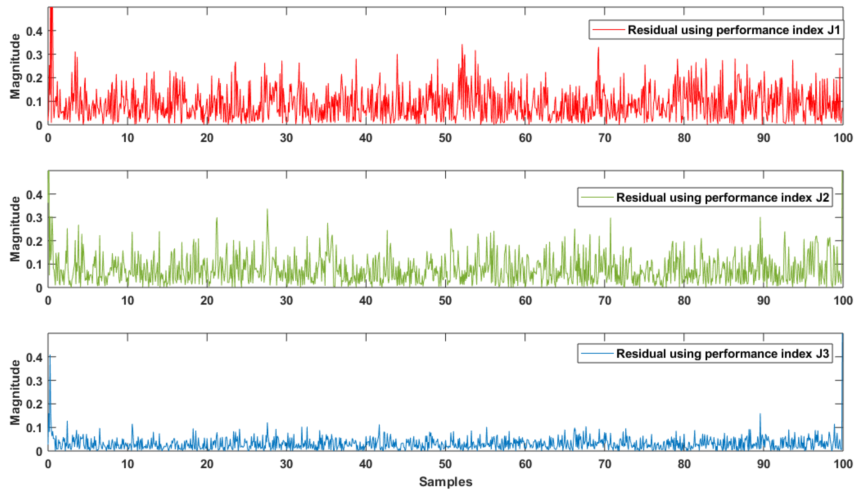
Now, 1200 samples are collected with sampling time of $T_s=0.1$ s. With $s_f=8$, $n=4$, the identified parity space ${\Psi }^{\perp }\in {\Re }^{12\times 16}$ and ${\Psi }^{\perp }{M}_{us}\in {\Re }^{12\times 16}$. Now, based on Equation (21), three different residuals are constructed using index (16), (17) and (19). The generated residuals are shown in Figure 3.

Various types of faults could occur during the operational state of the induction motor, including insulation breaking of the stator field winding, excessive current increase due to overloading, measurement devices such as ampere/volt meter could become defective, and supply voltage (modeled as an actuator) could become defective in the case of an unreliable power source. The profile of fault could be step, ramp, sinusoidal, etc., based on the conditions and nature of faulty components in the motor.

The computed variance for generated residuals is var$\left({{\rm Y}}_{J_1}\right)$ = 0.0133, var$\left({{\rm Y}}_{J_2}\right)$ = 0.0103 and var$\left({{\rm Y}}_{J_3}\right)$ = 0.0075, which shows the reduction of noise power in residual computed through the proposed index in the absence of a fault.

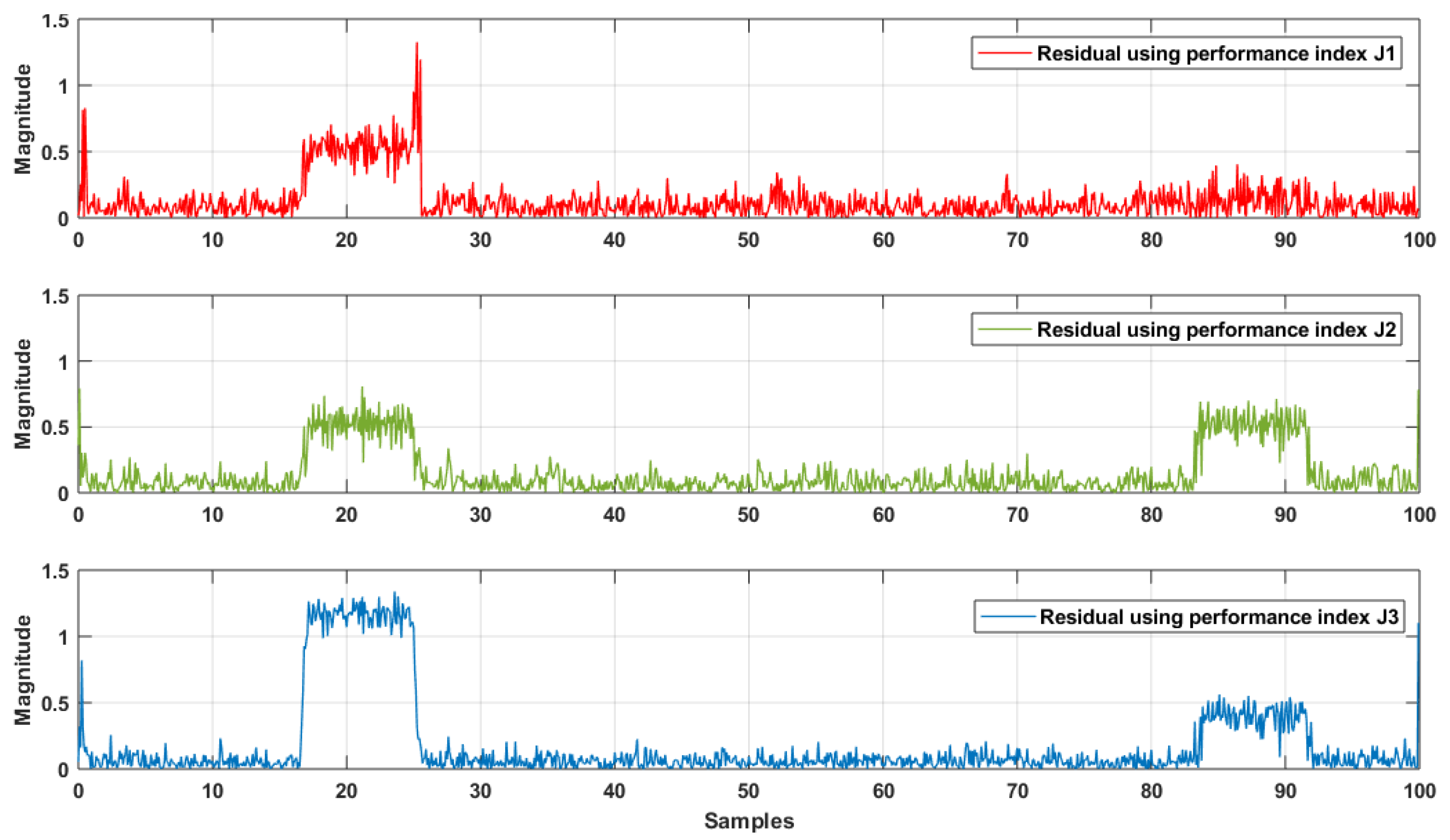
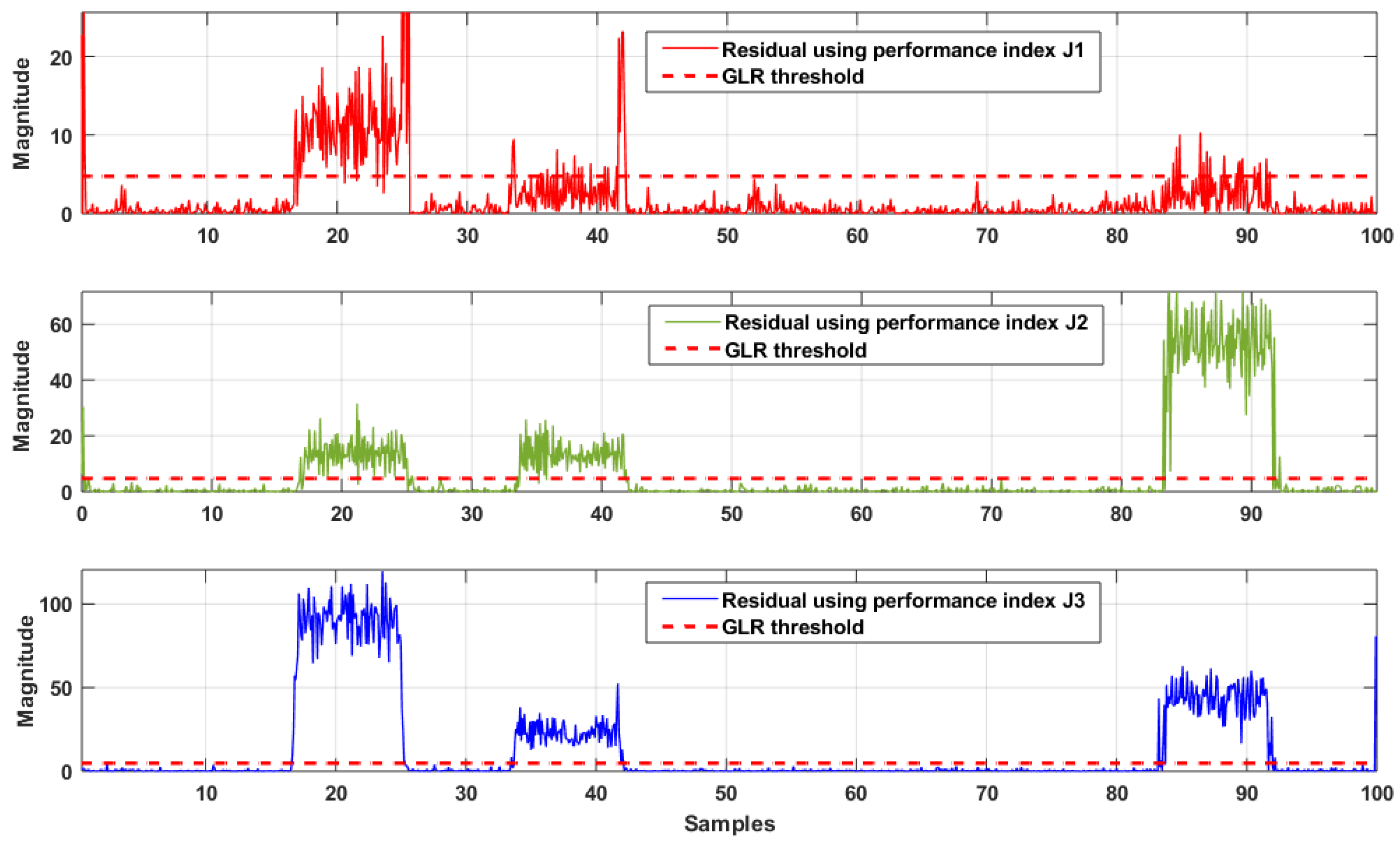
Consider the representation of faults as

$$\begin{array}{c}\hfill \begin{array}{cc}& f_1\stackrel{}{\to }faultinstatorvoltagesq-axis\left(v_q\right)\hfill \\ & f_2\stackrel{}{\to }faultinstatorvoltagesd-axis\left(v_d\right)\hfill \\ & f_3\stackrel{}{\to }faultinstatorcurrentq-axis\left(i_q\right)\hfill \\ & f_4\stackrel{}{\to }faultinstatorcurrentd-axis\left(i_d\right)\hfill \end{array}\end{array}$$

A pulse fault is introduced in the actuator 1 (17–25 s) and sensor 2 (83–92 s), and the resultant residual using $J_1$, $J_2$ and $J_3$ is shown in Figure 4.

Performance of the residual generator is also estimated by measuring the standard deviation and variance of generated residuals. Statistical data for residuals obtained using performance index $J_1$, $J_2$ and $J_3$ are shown in

Table 4. Statistics for indices $J_1$, $J_2$ and $J_3$.

	${\mathsf{{\rm Y}}}_{{\mathit{J}}_1}$	${\mathsf{{\rm Y}}}_{{\mathit{J}}_2}$	${\mathsf{{\rm Y}}}_{{\mathit{J}}_3}$
variance	0.0242	0.0327	0.0992
standard deviation	0.1556	0.1809	0.3151

.

From Table 4 it is clear the $J_2$ performs better than $J_1$ due to more variance and detectability. Similarly, statistical data for $J_3$ are shown in Table 4 and also show that the standard deviation and variance of generated residual are greater than $J_1$ and $J_2$, which is also the reason for better detectability of faults. The false alarm rate (FAR) and false detection rate (FDR) for performance index $J_1$, $J_2$ and $J_3$ are shown in

Table 5. FAR and FDR for indices $J_1$, $J_2$ and $J_3$.

	${\mathit{J}}_1$	${\mathit{J}}_2$	${\mathit{J}}_3$
FAR	4.27	1.63	0.85
FDR	82.53	97.61	98.88

.

Fault Isolation

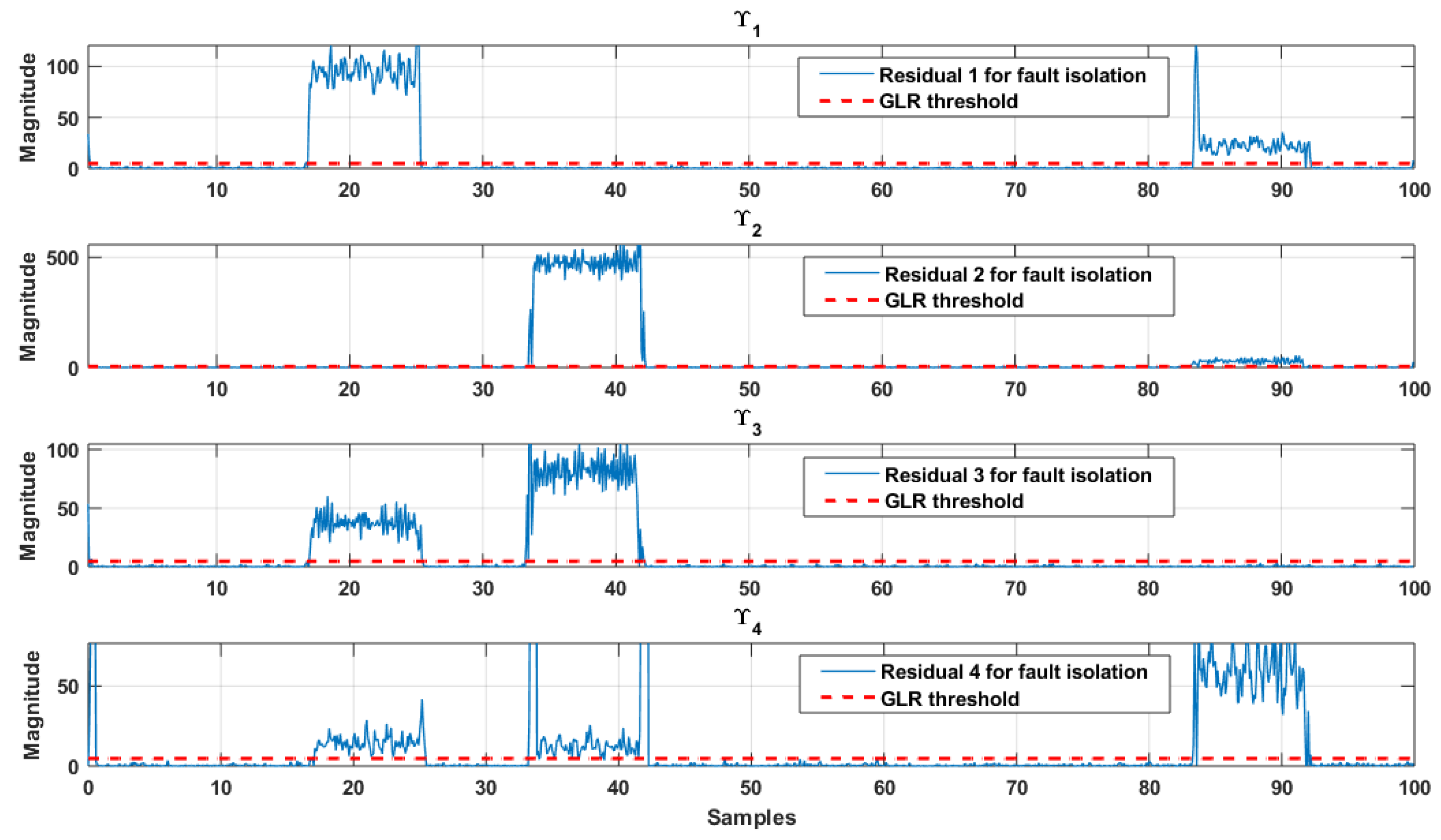
In three phase induction motor (SG-2672), there are two sensors and two actuator faults. The current in the $d-q$ axis is modeled as sensors 1 and 2, respectively, while the applied AC power supply for the $d-q$ axis is modeled as actuators 1 and 2, respectively. Applying Algorithms 1 and 2 would indicate the presence of the fault in the motor, but it would not specify the location of the faulty component. For that purpose, we would use a modified isolation procedure in Algorithms 3 and 4 based on perfect unknown input decoupling.

Parity spaces, ${\Psi }^{\perp }$ and ${\Psi }^{\perp }{M}_{us}$, obtained using Algorithms 1 and 2, are being used for actuator and sensor fault isolation using proposed robust parity vectors $l_{s,act,i}$ and $l_{s,sen,i}$, respectively.

Since m = 2 and $k_f=4$, a total of four residuals ${{\rm Y}}_1$, ${{\rm Y}}_2$, ${{\rm Y}}_3$, ${{\rm Y}}_4$ are generated based on ${}^4{C}_2$.

Furthermore, representing the residual as a function of faults as in Equation (28),

$$\begin{array}{c}\hfill \begin{array}{cc}\hfill {{\rm Y}}_1\left(k\right)& =F(f_1,f_3,f_4)\hfill \\ \hfill {{\rm Y}}_2\left(k\right)& =F(f_2,f_3,f_4)\hfill \\ \hfill {{\rm Y}}_3\left(k\right)& =F(f_1,f_2,f_3)\hfill \\ \hfill {{\rm Y}}_4\left(k\right)& =F(f_1,f_2,f_4)\hfill \end{array}\end{array}$$

(28)

A fault is introduced in the d-q axis of stator voltages (actuator 1, 2) and d-axis stator current for different time intervals, The faults are then detected online using Algorithm 2, and residual is evaluated based on the GLR threshold as shown in Figure 5. Furthermore, using Algorithm 3 and 4, residuals are constructed for indication of faulty components as shown in Figure 6. Now, at any instant, a decision about faults in specific components could be made using Table 3. It is evident from the figure that faults have occurred in stator voltages $(v_q,v_d)$ and current $\left(i_q\right)$ during specified time intervals.

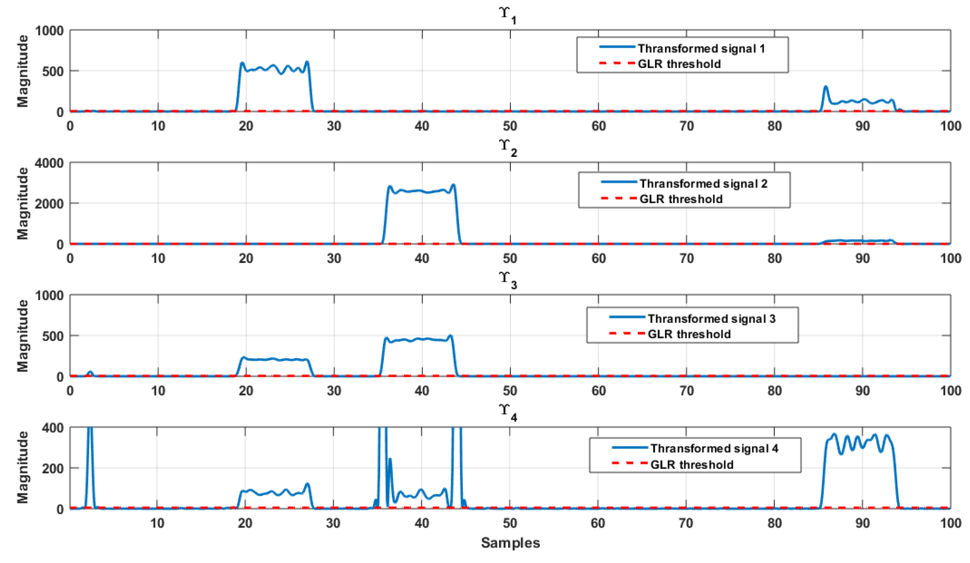
Generally, the nature of the faults is of low frequency so applying wavelet transform and keeping only approximate coefficients (containing lower frequencies of the residual) could reduce the false alarm rate as shown in Figure 7.

7. Conclusions

In this paper, we have presented a robust data-driven fault detection and isolation scheme for the systems with unknown dynamics. The proposed scheme showed robustness against sensor noise and actuator disturbances. The existing parity vector identification methodology is modified with the proposed performance index for a simultaneous increase in sensitivity towards faults and robustness against disturbances. Generated robust parity space is further used for the residual generation, which is further post-processed by wavelet transformation. Compared with previously defined performance indexes, our scheme with the proposed performance index has shown better statistics of reduced false alarm rate and increased false detection rate. An unknown input decoupling-based fault isolation procedure is adopted to designate the fault location. This procedure is also modified with our performance index to enhance sensitivity towards faults and considerably reduce the effect of noise on residuals compared to previously proposed indexes. Wavelet transform is used to discard the high-frequency content of the residual to further enhance FDR. The robust data-driven fault detection and isolation scheme is applied to the experimental setup of an induction motor in the lab. Obtained results showed the efficacy of the proposed fault diagnosis system.

8. Limitations

The proposed methodology is proved to be more effective, especially for linear dynamic systems. The less online computation and reduced false alarm rate are the added benefits of the designed scheme. Meanwhile, it is observed that the proposed strategy has limited efficacy for the highly nonlinear dynamic system as it uses a linear dynamic approach for subspace identification. In addition, for modern large-scale industrial processes, having many sensors makes the task of health monitoring very complex and expensive simultaneously. It demands key performance indicators based on fault diagnosis for alarm management to eradicate redundant alarms.

9. Future Work

Our work on a robust data-driven method can be further used for fault identification and fault tolerant control systems as these are also vital to guarantee the process’s sub-optimal function in the fault’s existence.

References

1. Isermann, R. Fault-Diagnosis Systems: An Introduction from Fault Detection to Fault Tolerance; Springer Science & Business Media: Berlin/Heidelberg, Germany, 2006. [Google Scholar]
2. Blanke, M.; Kinnaert, M.; Lunze, J.; Staroswiecki, M.; Schröder, J. Diagnosis and Fault-Tolerant Control; Springer: Berlin/Heidelberg, Germany, 2006; Volume 2. [Google Scholar]
3. Ding, S.X. Model-Based Fault Diagnosis Techniques: Design Schemes, Algorithms, and Tools; Springer Science & Business Media: Berlin/Heidelberg, Germany, 2008. [Google Scholar]
4. Gertler, J. Fault Detection and Diagnosis in Engineering Systems; Routledge: London, UK, 2017. [Google Scholar]
5. Abbasi, M.A.; Khan, A.Q.; Abid, M.; Mustafa, G.; Mehmood, A.; Luo, H.; Yin, S. Parity-based robust data-driven fault detection for nonlinear systems using just-in-time learning approach. Trans. Inst. Meas. Control 2020, 42, 1690–1699. [Google Scholar] [CrossRef]
6. Khan, A.S.; Khan, A.Q.; Iqbal, N.; Mustafa, G.; Abbasi, M.A.; Mahmood, A. Design of a computationally efficient observer-based distributed fault detection and isolation scheme in second-order networked control systems. ISA Trans. 2022, 128, 229–241. [Google Scholar] [CrossRef]
7. Ahmad, M.; Mohd-Mokhtar, R. A Survey on Model-based Fault Detection Techniques for Linear Time-Invariant Systems with Numerical Analysis. Pertanika J. Sci. Technol. 2022, 30, 53–78. [Google Scholar] [CrossRef]
8. Song, J.; He, X. Model-based fault diagnosis of networked systems: A survey. Asian J. Control. 2021, 24, 526–536. [Google Scholar] [CrossRef]
9. Bernardi, E. Fault-tolerant Model-based Predictive Control Applied to Industrial Processes. Ph.D. Thesis, Universidad Autónoma de Yucatán Sábado, Mérida, Mexico, 2021. [Google Scholar]
10. Naderi, E.; Khorasani, K. A data-driven approach to actuator and sensor fault detection, isolation and estimation in discrete-time linear systems. Automatica 2017, 85, 165–178. [Google Scholar] [CrossRef] [Green Version]
11. Paya, B.; Esat, I.; Badi, M. Artificial neural network based fault diagnostics of rotating machinery using wavelet transforms as a preprocessor. Mech. Syst. Signal Process. 1997, 11, 751–765. [Google Scholar] [CrossRef]
12. Ma, S.; Cai, W.; Liu, W.; Shang, Z.; Liu, G. A lighted deep convolutional neural network based fault diagnosis of rotating machinery. Sensors 2019, 19, 2381. [Google Scholar] [CrossRef] [PubMed] [Green Version]
13. Wilhelm, Y.; Reimann, P.; Gauchel, W.; Mitschang, B. Overview on hybrid approaches to fault detection and diagnosis: Combining data-driven, physics-based and knowledge-based models. Procedia CIRP 2021, 99, 278–283. [Google Scholar] [CrossRef]
14. Li, Z.; Gao, Y.; Zhang, X.; Wang, B.; Ma, H. A Model-Data-Hybrid-Driven Diagnosis Method for Open-Switch Faults in Power Converters. IEEE Trans. Power Electron. 2021, 36, 4965–4970. [Google Scholar] [CrossRef]
15. Abbasi, M.A.; Khan, A.Q.; Mustafa, G.; Abid, M.; Khan, A.S.; Ullah, N. Data-driven fault diagnostics for industrial processes: An application to Penicillin fermentation process. IEEE Access 2021, 9, 65977–65987. [Google Scholar] [CrossRef]
16. Argawal, R.; Kalel, D.; Harshit, M.; Domnic, A.D.; Singh, R.R. Sensor Fault Detection using Machine Learning Technique for Automobile Drive Applications. In Proceedings of the 2021 National Power Electronics Conference (NPEC), Bhubaneswar, India, 15–17 December 2021; pp. 1–6. [Google Scholar]
17. Liu, X.; Zhou, Q.; Zhao, J.; Shen, H.; Xiong, X. Fault diagnosis of rotating machinery under noisy environment conditions based on a 1-D convolutional autoencoder and 1-D convolutional neural network. Sensors 2019, 19, 972. [Google Scholar] [CrossRef] [PubMed] [Green Version]
18. Wang, Y.; Zheng, D.; Jia, R. Fault Diagnosis Method for MMC-HVDC Based on Bi-GRU Neural Network. Energies 2022, 15, 994. [Google Scholar] [CrossRef]
19. Yin, Shen Data-Driven Design of Fault Diagnosis Systems. Ph.D. Thesis, Universität Duisburg-Essen, Duisburg, Germany, 2012.
20. Daemi, A.; Gopaluni, B.; Huang, B. Process Monitoring using Domain-Adversarial Probabilistic Principal Component Analysis: A Transfer Learning Framework. IEEE Trans. Ind. Inform. 2022; Early Access. [Google Scholar] [CrossRef]
21. Nguyen, V.H.; Golinval, J.C. Fault detection based on kernel principal component analysis. Eng. Struct. 2010, 32, 3683–3691. [Google Scholar] [CrossRef]
22. Lee, G.; Han, C.; Yoon, E.S. Multiple-fault diagnosis of the Tennessee Eastman process based on system decomposition and dynamic PLS. Ind. Eng. Chem. Res. 2004, 43, 8037–8048. [Google Scholar] [CrossRef]
23. Muradore, R.; Fiorini, P. A PLS-based statistical approach for fault detection and isolation of robotic manipulators. IEEE Trans. Ind. Electron. 2011, 59, 3167–3175. [Google Scholar] [CrossRef]
24. Zhang, Y.; Teng, Y.; Zhang, Y. Complex process quality prediction using modified kernel partial least squares. Chem. Eng. Sci. 2010, 65, 2153–2158. [Google Scholar] [CrossRef]
25. Dong, J. Data Driven Fault Tolerant Control: A Subspace Approach. Ph.D. Thesis, Delft University of Technology, Delft, The Netherlands, 2009. [Google Scholar]
26. Ding, S.; Zhang, P.; Naik, A.; Ding, E.; Huang, B. Subspace method aided data-driven design of fault detection and isolation systems. J. Process Control 2009, 19, 1496–1510. [Google Scholar] [CrossRef]
27. Wang, Y.; Ma, G.; Ding, S.X.; Li, C. Subspace aided data-driven design of robust fault detection and isolation systems. Automatica 2011, 47, 2474–2480. [Google Scholar] [CrossRef]
28. Peng, K.; Wang, M.; Dong, J. Event-triggered fault detection framework based on subspace identification method for the networked control systems. Neurocomputing 2017, 239, 257–267. [Google Scholar] [CrossRef]
29. Van Overschee, P.; De Moor, B. Subspace Identification for Linear Systems: Theory-Implementation-Applications; Springer Science & Business Media: Berlin/Heidelberg, Germany, 2012. [Google Scholar]
30. Ding, S.X. Data-Driven Design of Fault Diagnosis and Fault-Tolerant Control Systems; Springer: Berlin/Heidelberg, Germany, 2014. [Google Scholar]
31. Yin, S.; Ding, S.X.; Haghani, A.; Hao, H.; Zhang, P. A comparison study of basic data-driven fault diagnosis and process monitoring methods on the benchmark Tennessee Eastman process. J. Process Control 2012, 22, 1567–1581. [Google Scholar] [CrossRef]
32. Hussain, A.; Khan, A.Q.; Abid, M. Robust fault detection using subspace aided data driven design. Asian J. Control 2016, 18, 709–720. [Google Scholar] [CrossRef]
33. Yin, S.; Li, X.; Gao, H.; Kaynak, O. Data-based techniques focused on modern industry: An overview. IEEE Trans. Ind. Electron. 2014, 62, 657–667. [Google Scholar] [CrossRef]
34. Wei, X.; Verhaegen, M.; van Engelen, T. Sensor fault detection and isolation for wind turbines based on subspace identification and Kalman filter techniques. Int. J. Adapt. Control Signal Process. 2010, 24, 687–707. [Google Scholar] [CrossRef]
35. Dong, J.; Verhaegen, M. Data driven fault detection and isolation of a wind turbine benchmark. IFAC Proc. Vol. 2011, 44, 7086–7091. [Google Scholar] [CrossRef] [Green Version]
36. Kumar, R.; Cirrincione, G.; Cirrincione, M.; Tortella, A.; Andriollo, M. Induction Machine Fault Diagnosis Using Stator Current Subspace Spectral Estimation. In Proceedings of the 2018 21st International Conference on Electrical Machines and Systems (ICEMS), Jeju, Korea, 7–10 October 2018; pp. 2565–2570. [Google Scholar]
37. Tariq, M.F.; Khan, A.Q.; Abid, M.; Mustafa, G. Data-Driven Robust Fault Detection and Isolation of Three-Phase Induction Motor. IEEE Trans. Ind. Electron. 2018, 66, 4707–4715. [Google Scholar] [CrossRef]
38. Crowder, R. 7—Induction motors. In Electric Drives and Electromechanical Systems, 2nd ed.; Crowder, R., Ed.; Butterworth-Heinemann: Oxford, UK, 2020; pp. 187–207. [Google Scholar] [CrossRef]
39. Hutasuhut, A.A.; Pasaribu, F.I. Design of Motor Induction 3-Phase from Waste Industry to Generator for Microhydro at Isolated Village; IOP Conference Series; Materials Science and Engineering; IOP Publishing: Bristol, UK, 2017; Volume 237, p. 012021. [Google Scholar]
40. Kakosimos, P.E.; Sarigiannidis, A.G.; Beniakar, M.E.; Kladas, A.G.; Gerada, C. Induction motors versus permanent-magnet actuators for aerospace applications. IEEE Trans. Ind. Electron. 2013, 61, 4315–4325. [Google Scholar] [CrossRef]
41. Siddique, A.; Yadava, G.; Singh, B. A review of stator fault monitoring techniques of induction motors. IEEE Trans. Energy Convers. 2005, 20, 106–114. [Google Scholar] [CrossRef]
42. Siddiqui, K.M.; Sahay, K.; Giri, V. Health monitoring and fault diagnosis in induction motor-a review. Int. J. Adv. Res. Electr. Electron. Instrum. Eng. 2014, 3, 6549–6565. [Google Scholar]
43. Skowron, M.; Orlowska-Kowalska, T.; Wolkiewicz, M.; Kowalski, C.T. Convolutional neural network-based stator current data-driven incipient stator fault diagnosis of inverter-fed induction motor. Energies 2020, 13, 1475. [Google Scholar] [CrossRef]
44. Dai, X.; Gao, Z. From model, signal to knowledge: A data-driven perspective of fault detection and diagnosis. IEEE Trans. Ind. Inform. 2013, 9, 2226–2238. [Google Scholar] [CrossRef] [Green Version]
45. Gandhi, A.; Corrigan, T.; Parsa, L. Recent advances in modeling and online detection of stator interturn faults in electrical motors. IEEE Trans. Ind. Electron. 2010, 58, 1564–1575. [Google Scholar] [CrossRef]
46. Rodriguez-Blanco, M.A.; Golikov, V.; Vazquez-Avila, J.L.; Samovarov, O.; Sanchez-Lara, R.; Osorio-Sánchez, R.; Pérez-Ramírez, A. Comprehensive and Simplified Fault Diagnosis for Three-Phase Induction Motor Using Parity Equation Approach in Stator Current Reference Frame. Machines 2022, 10, 379. [Google Scholar] [CrossRef]
47. Sheikh, M.A.; Bakhsh, S.T.; Irfan, M.; Nor, N.b.M.; Nowakowski, G. A Review to Diagnose Faults Related to Three-Phase Industrial Induction Motors. J. Fail. Anal. Prev. 2022, 22, 1546–1557. [Google Scholar] [CrossRef]
Figure 1. Experimental setup of Industrial drive (SE2672-3G).
Electronics 11 03858 g001
Figure 2. Subspace identification based diagnostic scheme.
Electronics 11 03858 g002
Figure 3. Residual with no faults.
Electronics 11 03858 g003
Figure 4. Residual with stator current ( i q ) and stator voltage ( v d ) faults.
Electronics 11 03858 g004
Figure 5. Residual with stator voltages ( v q , v d ) and current ( i d ) faults.
Electronics 11 03858 g005
Figure 6. Fault isolation for stator voltages ( v q , v d ) and current ( i d ) faults.
Electronics 11 03858 g006
Figure 7. Fault isolation for stator voltages ( v q , v d ) and current ( i q ) faults with wavelet transformation.
Electronics 11 03858 g007