Article

SlowFast Action Recognition Algorithm Based on Faster and More Accurate Detectors

1
Chongqing Key Laboratory of Nonlinear Circuits and Intelligent Information Processing, College of Electronic and Information Engineering, Southwest University, Chongqing 400044, China
2
College of Computer Science and Engineering, Chongqing University of Technology, Chongqing 400000, China
*
Author to whom correspondence should be addressed.
Electronics 2022, 11(22), 3770; https://doi.org/10.3390/electronics11223770
Submission received: 5 October 2022 / Revised: 10 November 2022 / Accepted: 15 November 2022 / Published: 16 November 2022
(This article belongs to the Special Issue Convolutional Neural Networks and Vision Applications, Volume II)

Abstract

:
Object detection algorithms play a crucial role in other vision tasks. This paper finds that the action recognition algorithm SlowFast’s detection algorithm FasterRCNN (Region Convolutional Neural Network) has disadvantages in terms of both detection accuracy and speed and the traditional IOU (Intersection over Union) localization loss is difficult to make the detection model converge to the minimum stability point. To solve the above problems, the article uses YOLOv3 (You Only Look Once), YOLOX, and CascadeRCNN to improve the detection accuracy and speed of the SlowFast. This paper proposes a new localization loss function that adopts the Lance and Williams distance as a new penalty term. The new loss function is more sensitive when the distance difference is smaller, and this property is very suitable for the late convergence of the detection model. The experiments were conducted on the VOC (Visual Object Classes) dataset and the COCO dataset. In the final videos test, YOLOv3 improved the detection speed by 10.5 s. CascadeRCNN improved by 3.1%AP compared to FasterRCNN in the COCO dataset. YOLOX’s performance on the COCO dataset is also mostly better than that of FasterRCNN. The new LIOU (Lance and Williams Distance Intersection over Union) localization loss function performs better than other loss functions in the VOC dataset. It can be seen that improving the detection algorithm of the SlowFast seems to be crucial and the proposed loss function is indeed effective.

1. Introduction

RGB video action recognition algorithms can be divided into CNN-based algorithms, RNN-based (Recurrent Neural Network) algorithms, and algorithms based on other structures. CNN-based algorithms can be divided into four types according to the encoding of Spatio-temporal information methods. The first one extracts features by a convolutional neural network and then fuses temporal information. For example, Karpathy [1] proposed four Spatio-temporal fusion methods that can obtain more global information from the Spatio-temporal dimension at higher layers. The second method applies convolutional operations to temporal information extraction as well, resulting in 3D convolution that can extract features from both Spatio-temporal dimensions, and the superiority of this 3D convolution for temporal information extraction has been demonstrated in experiments. Tran’s [2] proposed C3D (Convolutional 3D) network and Hung-Cuong Nguyen’s [3] proposed end-to-end framework for automatic 3D human pose estimation are both based on this approach. Of course, this method also has a disadvantage, which is that the extraction of long video sequence features is not ideal. To solve this disadvantage, Varol [4] proposed Long-term Temporal Convolution (LTC), but LTC again leads to the problem of decreasing spatial resolution. The third method encodes the videos as a dynamic image containing spatial and temporal information and then applies a CNN-based network for recognition, such methods proposed by Bilen [5] and Fernando [6] and fine-tuned on ImageNet datasets [7]. All three methods mentioned above use one network to extract Spatio-temporal information, while the fourth method aims to extract temporal and spatial information separately and design the network with two streams and multi-stream approaches. Simonyan and Zisserman [8] designed the classical two streams network. In this two streams network, RGB video frames are used to extract spatial information, optical streams are used as input information to extract temporal features, and the temporal information and spatial information are finally fused. Inspired by the residual network, Feichtenhofer [9] created links during the two streams’ processing, allowing Spatio-temporal information to interact with each other.
For RNN-based algorithms, Baccouche [10] proposed a combination of LSTM (Long Short-Term Memory) and 3D convolution method to solve the problem in behavioral analysis, and trained in both networks separately. In contrast, Donahue [11] proposed a LRCN (Long-term Recurrent Convolutional Network) with direct end-to-end training. In 2016, Pigou [12] proposed a neural network combining temporal convolution and bidirectional LSTM with end-to-end training for gesture recognition. In 2017, Du [13] proposed a neural RPAN (Recurrent Pose-Attention Network) in videos that adaptively learns highly discriminative pose-related features predicted by the action of each step of the LSTM. Recently, Sun [14] proposed a L2STM (Lattice-LSTM) network, this approach significantly increased the long-time modeling capability without significantly increasing the complexity of the model, and solved the problem of unstable long-term motion. In contrast to previous approaches using only feedforward connections, Shi [15] proposed a deep network based on biological mechanisms in 2017, called ShuttleNet.1. Unlike traditional RNN, all the processors in ShuttleNet.1 mimic the circular linkages of the human brain. In this way, the processors share multiple paths in the loop connections. The best information flow path is then selected using the attention mechanism.
In addition to the main CNN-based algorithms and RNN-based algorithms, some network models use other structures. Yan [16] proposed a three-layer autoencoder for capturing video motion, called Dynencoder. Dynencoder can successfully synthesize dynamic texture features, which is a concise method to represent video spatial and temporal information. Similarly, Srivastava [17] proposed the LSTM autoencoder model in 2015. The state of the encoder LSTM contains the appearance and dynamics of the input sequence, and the decoder LSTM accepts the output of the encoder LSTM to reconstruct the sequence. Inspired by GAN (Generative Adversarial Networks), Mathieu [18] trained multiscale convolutional neural networks with the adversarial mechanism. To balance the impact of the standard MSE (Mean Square Error) loss function, they proposed three complementary feature learning strategies, namely multiscale structures, adversarial training methods, and image gradient difference loss functions.
The time and space dimensions of the video space are not related. The video’s spatial information (e.g., type, color, texture, etc.) is updated very slowly, and the background in which the action appears does not change significantly because of the action change. The subject acting does not change its identity because of the action, and the hand is still a hand when it is waved. As the part of the executive action changes much faster than the subject, such as clapping, jumping, talking, etc., this part of the information is called temporal information, which is updated very quickly. Therefore, for the acquisition of dynamic information, it is better to handle the temporal dimension and spatial dimension separately, so that better results can be obtained.
SlowFast [19] is designed on this basis, which is the fourth CNN-based approach described in the previous section, see Figure 1, with two layers of channels separating temporal and spatial information. The upper path processes video frames with a low resolution and low frame rate, called SlowPath, to extract spatial information that changes slowly over time. The lower path processes the input video with a higher resolution and higher frame rate to extract the temporal information that changes rapidly over time, called FastPath. The slow and fast paths are connected by lateral connections, and the operational results of this combined two-channel processing information are classified by the fully connected layer to output the action information in the image.
SlowFast is a class of behavioral analysis algorithms based on object detection, so the detection algorithm determines the performance of the behavioral analysis algorithm, and the detection algorithm encapsulated by SlowFast is FasterRCNN [20]. The YOLOv3 [21] and YOLOX [22] algorithms modified in this paper is a simpler one-stage algorithms compared with the FasterRCNN algorithm. The two-stage [23] detection algorithm handles the detection problem in two stages, first generating regional proposals [24], and then classifying these regional proposals. They are often not sufficient for real-time detection scenarios due to their slow speed. The one-stage detection algorithm generates the category probability and location coordinate of the object directly without generating regional proposals. The final test results can be obtained directly after a single test, so it has a faster testing speed. CascadeRCNN [25] is a multi-stage algorithm, which is essentially an extension of FasterRCNN. The core idea is that the output of the detector of the current stage is used as the input of the detector of the next stage.
The localization loss in object detection is often used to describe the loss between the predicted bounding box and the ground truth. IOU loss [26] is one of the most representative localization loss functions, and the expression is as follows:
I o U l o s s = 1 A B A B
where A and B represent the area of the predicted bounding box and the ground truth, respectively. IOU loss reduces the loss value by increasing the overlap between the predicted bounding box and the ground truth during the iteration. In the later stage of training, the IOU loss loss value reaches a stable value, the overlap between the predicted bounding box and the ground truth is the highest, and the model has the best prediction effect. IOU loss subsequently developed GIOU loss (Generalized IOU) [27], DIOU loss (Distance IOU), CIOU loss (Complete IOU) [28] and EIOU loss (Efficient IOU) [29], but all these loss functions are defined based on Euclidean distance, which is not sensitive enough when the distance difference is small, and the model is difficult to converge to higher accuracy in the later stage of training. Therefore, this paper proposes to use the Lance and Williams Distance as a new penalty term of the loss function to increase the sensitivity of the model in the late training period, so that the model can converge to a higher accuracy.

2. Related Works and Methods

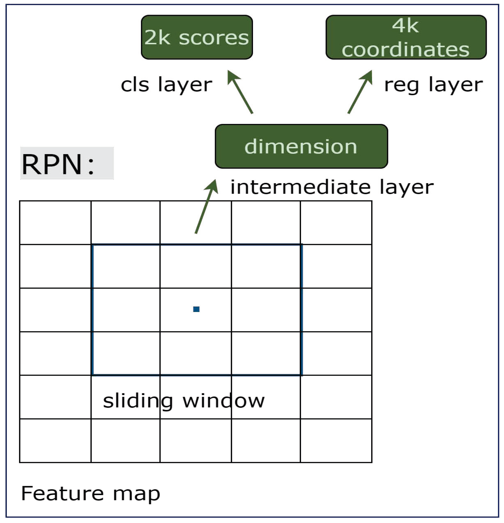
The FasterRCNN algorithm process can be divided into three steps, see Figure 2. First, the backbone network processes the input image to obtain the corresponding feature maps. Second uses the RPN (Region Proposal Network) structure to get the region proposals, and then maps the region proposals generated by the RPN structure to the feature maps to obtain the corresponding feature matrixes. Finally, each feature matrix is expanded into a 7 × 7 feature map by the ROI (Region Of Interest) pooling layer [30], and the generated feature maps are classified and output by the fully connected layer to obtain the prediction results. The RPN structure is illustrated in Figure 3. RPN replaces the original Selective Search algorithm by using a sliding window in the feature map generated by the backbone network, generating a one-dimensional vector at each position. The dimension of the one-dimensional vector elements matches the depth of the feature matrix output by the backbone. It then generates the object probabilities and the bounding box regression parameters through two fully connected layers. The 2k scores in the figure are the foreground and background probabilities generated for the k anchors. Each anchor generates 4 bounding box regression parameters, so there are 4k coordinates here.
The core idea of YOLO is to turn object detection into a regression problem, using the whole picture as the input to the network and just passing through a neural network to get the location and the category of the bounding box [31,32,33]. In Figure 2, the feature extraction network of YOLOv3 is Darknet-53. The multilayer Conv with Concat and Up (upsampling) in the figure constitutes the FPN (Feature Pyramid Network) structure [21] of YOLOv3. YOLOv3 uses the FPN structure to implement multi-scale prediction, which is then post-processed to obtain three scales of output Y1, Y2, and Y3. YOLOX is an improved version of YOLOv3, but they have similar modules and the same processing flow.
CascadeRCNN, as an extension of FasterRCNN, has a workflow similar to that of FasterRCNN. In Figure 2, B0 represents the proposal generated by the RPN structure. B and C represent the bounding box and classification score of each pooling layer output respectively, and the number represents the serial number of the pooling layer, e.g., B1 represents the bounding box of the first pooling layer output. Firstly, feature maps are generated through the backbone. The first pooling layer uses feature maps and B0 to extract the feature of each Box and then performs classification regression to get B1 and category C1. The next pooling layer uses feature maps and the B1 generated by the previous stage and then performs classification regression to obtain B2 and category C2, and so on.
The detection results output by these four types of detectors are extracted into two sets of input data according to different frame rates. The low-frame-rate and low-resolution data are processed by SlowPath, and the high-resolution and high-frame-rate data are processed by FastPath. The features are fused by lateral connections between the two channels. The processed Spatio-temporal information features are then subjected to the global average pool, concate, and FC operations to output the corresponding action information.
The localization loss function proposed in the article is constructed based on EIOU, and the expression of EIOU is as follows.
E I O U l o s s = 1 I o U + ρ 2 b , b g t c 2 + ρ 2 w , w g t C w 2 + ρ 2 h , h g t C h 2
where ρ represents the Euclidean distance, w, h, and b represent the width, height, and centroid coordinates of the predicted bounding box, w g t , h g t , and b g t represent the width, height and centroid coordinates of ground truth, and C w , C h , and C represent the width, height, and diagonal length of the minimum outer rectangular frame, respectively. EIOU sufficiently considers the center point distance, overlap area, and edge length of the predicted bounding box and ground truth. However, EIOU still cannot avoid the drawbacks of Euclidean distance. The Euclidean distance does not provide the larger gradient when the distance difference between the predicted bounding box and ground truth is small, resulting in the model not converging to a lower stability point later in the training. Therefore, this paper proposes to use the Lance and Williams distance as a new penalty term for the localization loss to provide a larger gradient for the loss function at a later stage of training. The simplified Euclidean distance and Lance and Williams distance expressions are as follows.
ρ = ( b b g t ) 2 , L = 1 2 | b b g t | | b + b g t |
where L represents the Lance and Williams distance, ρ represents the Euclidean distance, and b and b g t represent the center point coordinates of the predicted bounding box and ground truth, respectively. The expressions for the derivatives of ρ and L are as follows.
d ρ b = 2 ( b b g t ) , d L b = b g t ( b + b g t ) 2 b b g t b g t ( b + b g t ) 2 b < b g t
It can be seen that b converges to b g t in the process, which is the later stage of model training. The gradient of the Euclidean distance converges to 0, while the gradient of the Lance and Williams distance converges to 1 4 b g t , and it can be seen that the Lance and Williams distance has a greater sensitivity of the loss function when the distance difference between the centroids is small.
From Equation (4), the gradient of the Euclidean distance becomes larger as the distance difference becomes larger, which is ideal for the optimization of the model. d L b is a monotonically decreasing function when b b g t and a monotonically increasing function when b< b g t . The gradient of the Lance and Williams distance becomes smaller as the distance difference becomes bigger, which is not following the basic properties of the loss function. At the early stage of the model training (where the distance difference between the centroids is assumed to be infinite means b = + or b g t = + ), the gradient d L b is equal to 0, and the optimization of the model is limited to stagnation. The Euclidean distance can be quickly regressed early in the training because of the huge gradient, but this is also prone to gradient explosion.
In order to neutralize the shortcomings of Euclidean distance and Lance and Williams distance, this paper adds a penalty term of Lance and Williams distance based on EIOU loss. The new localization loss function is called LIOU loss, and the specific expression is as follows.
L I O U l o s s = 1 I o U + ρ 2 b , b g t c 2 + ρ 2 w , w g t C w 2 + ρ 2 h , h g t C h 2 + 1 2 | x x g t | | x + x g t | + 1 2 | y y g t | | y + y g t |
where x and y represent the horizontal and vertical coordinates of the center point of the predicted bounding box, x g t and y g t represent the horizontal and vertical coordinates of the center point of the ground truth, respectively. LIOU loss is able to regress steadily and quickly in the early stage of model training, and does not have gradient explosion. In the later stage of model training, it still has certain optimization ability, and can avoid the loss from falling to a local minimum value and thus the phenomenon of optimization stagnation.

3. Experiments

The previous section discusses the related networks and the proposed new localization loss. This section will describe the relevant setup of the experiment, show the performance data of the new detector and the new loss function, compare them with other methods, and analyze and synthesizes the results.

3.1. Datasets

The experiments in this paper were built on the PASCAL VOC and COCO [34] datasets. The VOC dataset used in the experiments integrates VOC2007 [35] and VOC2012 [36] and contains 17,125 images. The division ratio of the training set and validation set is about 8:2, which are 13,870 and 3255 images respectively, and the metrics for the experiments are derived from the AP values of the validation set. The COCO dataset is a large, rich dataset of object detection, segmentation, and captioning. The training set in the COCO dataset used for the experiments contains 118,287 images, and the validation set includes 5000 images. The AP values of the experiments on the COCO dataset are from the validation set. Since the framework of the study in this paper addresses human movement, in addition to the experiments to validate the performance of the LIOU loss function using the VOC dataset with 20 common categories, the other experiments were conducted using the class “person”.

3.2. Experiment Settings

This paper has completed A total of four sets of experiments. The first three groups of experiments were conducted on two Quadro RTX 8000 GPUs and VOC dataset. YOLOv3 and FasterRCNN used DarkNet53 and ResNet50 [25] backbone networks, respectively. To ensure the objectivity of the experiments, both YOLOv3 and FasterRCNN used pre-trained models and trained them for 100 epochs. The training strategy was set to freeze the backbone network for the first 50 epochs and unfreeze the backbone network for the next 50 epochs. The feature extraction network does not change when the backbone of the model is frozen, and only fine—tunes the network. The second group of experiments used the strategy of training 15 epochs in the frozen backbone network and 15 epochs in the thawing phase. To demonstrate that the actual performance of LIOU loss is better than other localization loss functions. The third group of experiments was built on the YOLOX—S algorithm framework, and three classical IOU loss functions were selected to compare with LIOU loss. The experiments without using pre-trained models trained 300 epochs, and sgd was chosen as the optimizer, momentum was set to 0.937, and weight_decay was set to 5 × 10 4 . All other training parameters were kept consistent within the group for each set of experiments.
The fourth experiment tested YOLOv3, YOLOX, FasterRCNN, and CascadeRCNN on the COCO dataset, where YOLOv3 and YOLOX used DarkNet53 and CSPDarkNet53 as the backbone network respectively and FasterRCNN and CascadeRCNN used ResNet50 as the feature extraction network. The backbone networks all used pre-trained weights in the experiment. The experiment was trained for 5 epochs on one RTX2080Ti GPU and kept the other training parameters consistent.

3.3. Evaluation Metrics

The evaluation indicators these experiments use are AP (Average Precision), F1-score, Precision, Recall, and LAMR (Log-Average Miss Rate). The following are the formulae for Precision and Recall,
P r e c i s i o n = T P T P + F P , R e c a l l = T P T P + F N
where T P (True Positive) represents the predicted result and ground truth are positive samples. F P (False Positive) represents the predicted positive sample and ground truth is a negative sample, and F N (False Negative) represents the predicted negative sample is a positive sample. The curve consisting of Recall and Precision as horizontal and vertical coordinates is called the PR (Precision-Recall) curve, and the area of this curve is the AP value.
The experiments use six AP metrics. AP50 and AP75 are the AP values when the IOU threshold sets to 0.5 and 0.75, respectively, and AP0.50–0.95 is the average AP value at different IOU thresholds (from 0.50 to 0.95 with a step size of 0.05). These experiments calculate three types of AP values based on the area of different objects, APS, APM, and APL represent the AP values of small objects (area < 32²), medium objects (32² < area >96²), and large objects (area > 96²), respectively.
The F1-score is used to weigh the two quantities Precision and Recall to measure the goodness of the model. The larger the F1-score value, the better the model performance.
F 1 - s c o r e = 2 P R P + R
The LAMR value contains two concepts, FPPI (False Positive Per Image) and Miss Rate. The N in Equation (8) represents the amount of data in the dataset. The curve is plotted according to FPPI and Miss Rate, and the Miss Rate values are obtained at 9 FPPI values (within −2nd power of 10 to 0th power of 10 at uniform intervals in logarithmic space) and averaged to obtain the LAMR values. The smaller the LAMR indicator, the better the performance of the detector.
F P P I = F P N , M i s s R a t e = 1 R e c a l l

3.4. Results and Analysis

In Table 1, the experiment uses the COCO tool to calculate performance metrics. In Evaluation Time, YOLOv3 (Ours) takes only 1.92 s, and FasterRCNN takes 2.51 s, so YOLOv3 has gained a clear advantage in speed. For different IOU settings and sizes of targets’ impact for accuracy AP, from Table 1, it can be seen that FasterRCNN is only slightly behind in the detection accuracy of small objects (APS), but in the remaining five indexes there is a considerable improvement compared to YOLOv3. The main reason for this phenomenon may be that YOLOv3 is more tolerant of large object errors and more sensitive to deviations from small object regressions when making regression predictions. YOLOv3 does not filter the objects in the search phase unlike two-stage detection algorithms such as FasterRCNN, which results in poor accuracy in most cases. In Table 2, under the condition that the score threshold is equal to 0.5, although the F1-score and Precision values are lower than YOLOv3, FasterRCNN has higher AP50 and Recall than YOLOv3 (Ours), and better LAMR performance values than YOLOv3. It can be seen that the difference between YOLOv3 and FasterRCNN two types of detection algorithms is only that the former is faster and the latter is more accurate.
IOU, CIOU and EIOU are all localization loss functions constructed based on Euclidean distance, and most of their AP values are lower than LIOU as can be seen in Table 3. Particularly, LIOU is constructed based on EIOU with just the addition of the Lance and Williams distance as new penalty items. Therefore, it can be proved that the sensitivity of the Lance and Williams distance when the distance difference is small indeed help to optimize the model. LIOU loss combines the advantages of Euclidean distance and Lance and Williams distance, which can regress quickly in the early stage of model training without gradient explosion and can break the limit of local minima in the late stage of training, making the model converge at a lower stable point and achieve higher performance.
From Table 4, it can be seen that CascadeRCNN (ours) is higher than FasterRCNN for different kinds of AP values, except for the equal values of APS. This indicates that the cascade structure seems to facilitate the classification of the model. Meanwhile, YOLOv3 (ours) performs the worst in terms of detection accuracy, which proves the description in the previous paragraph of the article. That is, although YOLOv3 satisfies the real-time performance of detection, it is still inferior to FasterRCNN and CascadeRCNN in terms of accuracy. In addition, YOLOX also showed very good performance, with AP50 and APS having the best results compared to the other three. In general, SlowFast’s detection algorithm FasterRCNN fails to meet the requirements in terms of speed and accuracy, and improvements to the FasterRCNN framework seem to become necessary.

3.5. Action Recognition Effect

This section measures the performance data of SlowFast by applying four different detectors as shown in Table 5. The experiment evaluates the speed of the four detection algorithms by setting the bounding box obtained with an IOU of 0.9. In Table 5, this section takes 10 videos as the experiment and gets the average consumption time as the index. Nine of the videos are from the AVA dataset [37], each cut to 30s in length, and one video is from a shooting video, 31s in length. The intercepted image frames from the video are first detected and then analyzed for Spatio-temporal behavior. Combining Human Detection time and Spatio-temporal Action Detection time in Table 5, YOLOv3+SlowFast and YOLOX + SlowFast have similar processing speed, and CascadeRCNN+SlowFast and FasterRCNN + SlowFast consume similar processing time. YOLOv3+SlowFast significantly improves the processing time of the algorithm compared to FasterRCNN+SlowFast, which matches the advantage of the one-stage detection algorithm, which is to have a faster processing speed.
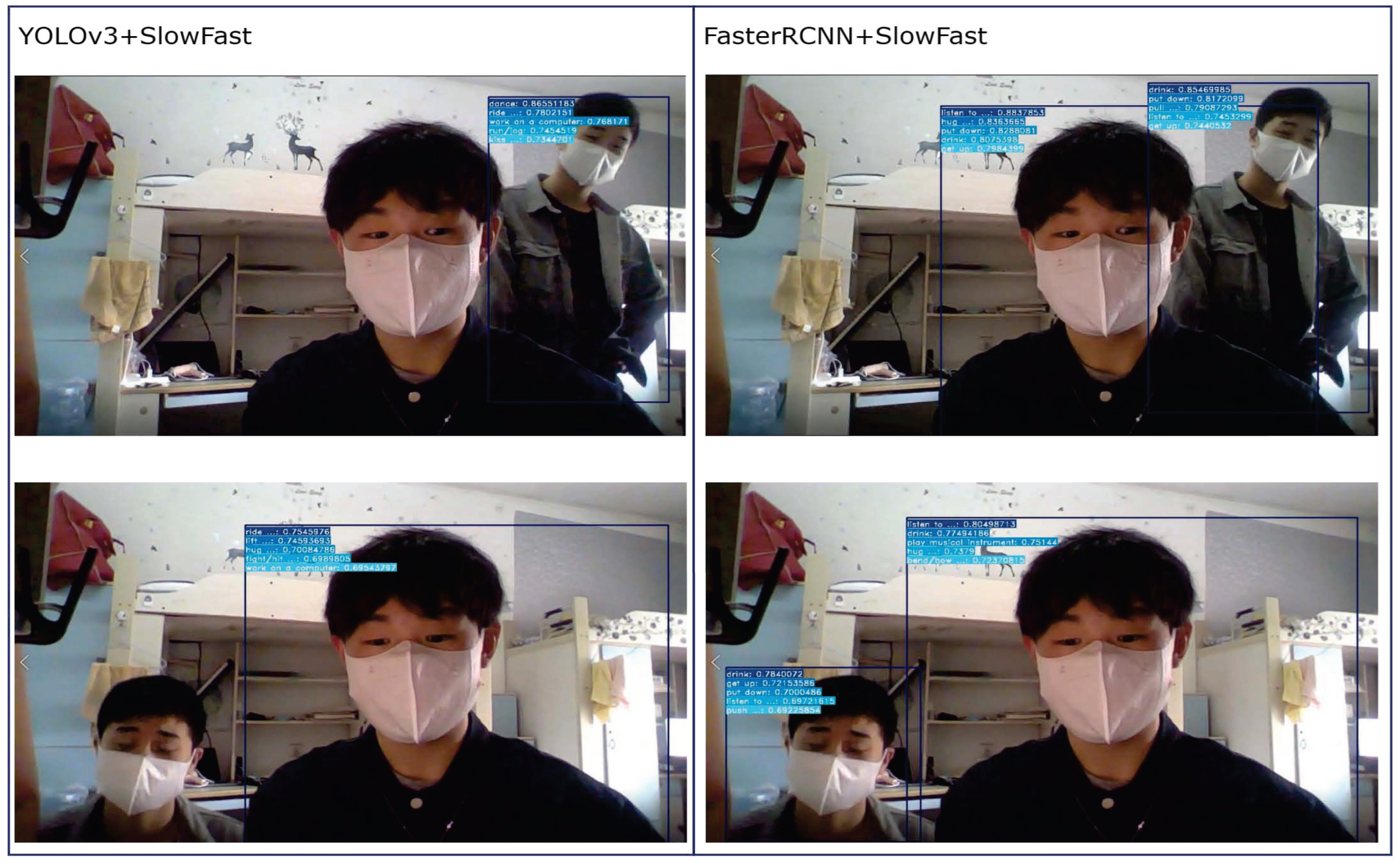
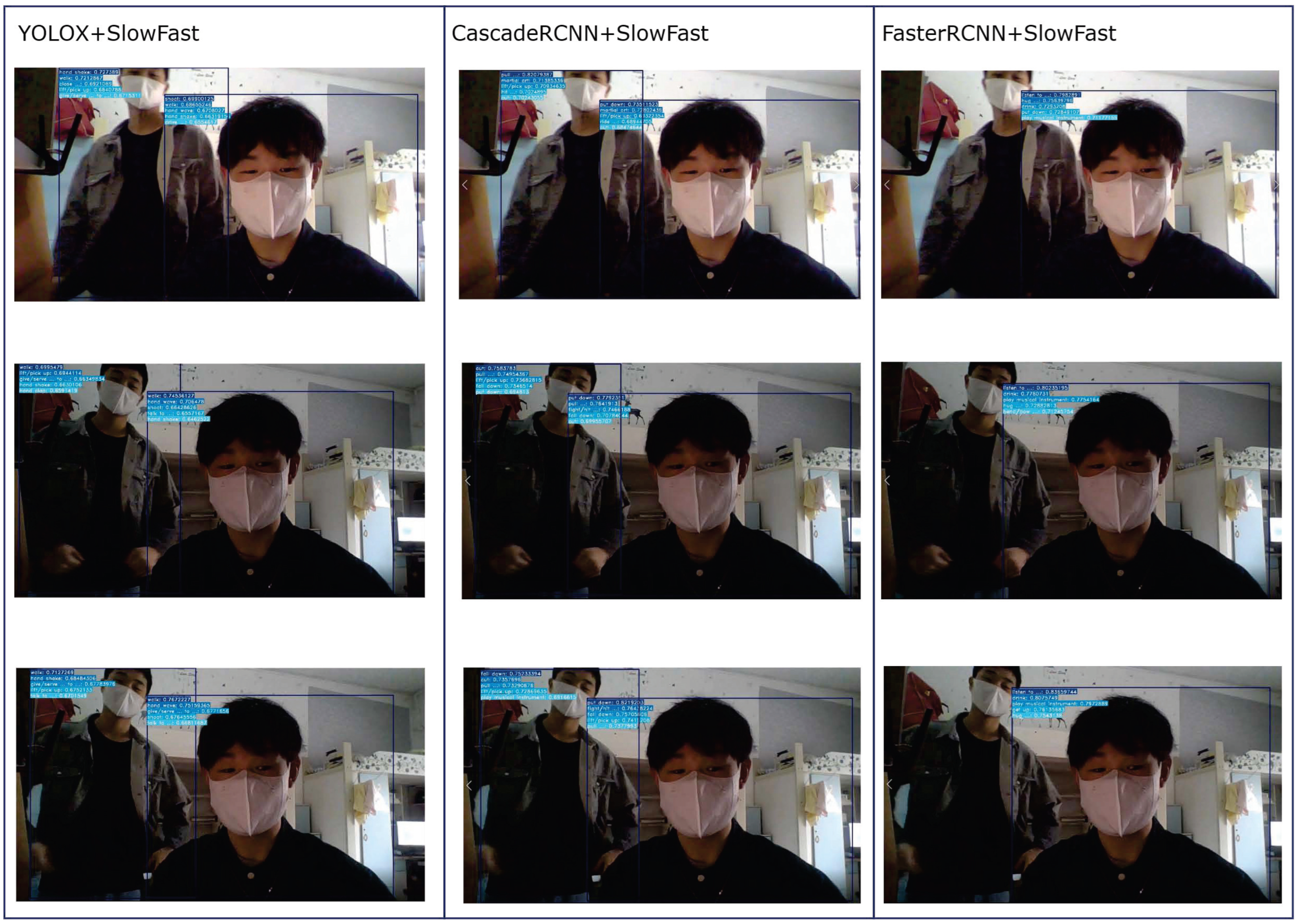
Figure 4 and Figure 5 show the same frame comparison of a 31 s shooting video behavior analysis test (The blue information in the upper box represents the corresponding behavior information and the confidence score). From Figure 4, it can be found that the detection accuracy of YOLOv3+SlowFast is lower than that of FasterRCNN+SlowFast, because the former detects only one person in the two frames in the figure, and the latter detects two persons. The same situation is can be found in Figure 5, where both CascadeRCNN+SlowFast and YOLOX+SlowFast show no missed detections, while FasterRCNN+SlowFast misses a person. In behavioral analysis, if the object is not detected, the corresponding action information cannot be obtained. From Figure 5, it can be concluded that YOLOX and CascadeRCNN meet the accuracy requirements of SlowFast better than FasterRCNN.

4. Conclusions

This study improves the accuracy or speed of action recognition by starting with object detection. Therefore, starting from the advantages and disadvantages of one-stage algorithms, two-stage algorithms, and multi-stage algorithms, this paper identifies four detection algorithms, YOLOv3, YOLOX, FasterRCNN, and CascadeRCNN, and combines them with the SlowFast action algorithm. The paper also proposes a new localization loss function LIOU to solve the problem that the traditional IOU loss function lacks sensitivity in the late training period, failing to converge to a lower stability point. According to the results on the VOC and COCO datasets, it can be demonstrated that SlowFast’s detection algorithm, in terms of detection speed and accuracy, can be improved. In general, YOLOv3+SlowFast can significantly increase detection speed with a small reduction in detection accuracy and can meet the requirements of industrial implementations. Similarly, CascadeRCNN+SlowFast can significantly improve detection accuracy and YOLOX+SlowFast outperforms the original SlowFast in terms of speed and accuracy. In addition, the paper demonstrates that the proposed LIOU loss function significantly outperforms other IOU loss functions in the framework of the YOLOX-based algorithm. In future work, our research directions will improve the detection performance of the detection algorithm in other aspects to improve the recognition accuracy or speed of the behavioral analysis algorithms.

Author Contributions

Conceptualization, W.Z. (Wei Zeng) and J.H.; methodology, W.Z. (Wei Zeng) and J.H.; software, W.Z. (Wei Zeng); validation, W.Z. (Wei Zeng); formal analysis, W.Z. (Wei Zeng) and J.H.; resources, W.Z. (Wei Zeng), J.H., W.Z. (Wei Zhang) and H.N.; data curation, W.Z. (Wei Zeng); writing—original draft preparation, W.Z. (Wei Zeng); writing—review and editing, W.Z. (Wei Zeng) and J.H.; visualization, W.Z. (Wei Zeng) and Z.F.; funding acquisition, J.H., W.Z. (Wei Zhang) and H.N. All authors have read and agreed to the published version of the manuscript.

Funding

This work is supported by Science and Technology Research Program of Chongqing Municipal Education Commission: KJQN201901133 and the Fundamental Research for the Central Universities, China (Project No. SWU020005).

Institutional Review Board Statement

This article does not contain any experiments with human or animal participants performed by any of the authors.

Informed Consent Statement

Informed consent was obtained from all individual participants included in the study.

Conflicts of Interest

The authors declare that they have no conflict of interest.

References

  1. Karpathy, A.; Toderici, G.; Shetty, S.; Leung, T.; Sukthankar, R.; Li, F.-F. Large-scale video classification with convolutional neural networks. In Proceedings of the IEEE Conference on Computer Vision and Pattern Recognition (CVPR), Columbus, OH, USA, 23–28 June 2014; pp. 1725–1732. [Google Scholar]
  2. Tran, D.; Bourdev, L.; Fergus, R.; Torresani, L.; Paluri, M. Learning spatiotemporal features with 3d convolutional networks. In Proceedings of the IEEE International Conference on Computer Vision (ICCV), Santiago, Chile, 7–13 December 2015; pp. 4489–4497. [Google Scholar]
  3. Nguyen, H.C.; Nguyen, T.H.; Scherer, R.; Le, V.H. Unified End-to-End YOLOv5-HR-TCM Framework for Automatic 2D/3D Human Pose Estimation for Real-Time Applications. Sensors 2022, 22, 5419. [Google Scholar] [CrossRef] [PubMed]
  4. Varol, G.; Laptev, I.; Schmid, C. Long-term temporal convolutions for action recognition. IEEE Trans. Pattern Anal. Mach. Intell. 2017, 40, 1510–1517. [Google Scholar] [CrossRef] [PubMed] [Green Version]
  5. Bilen, H.; Fernando, B.; Gavves, E.; Vedaldi, A.; Gould, S. Dynamic image networks for action recognition. In Proceedings of the IEEE Conference on Computer Vision and Pattern Recognition, Las Vegas, NV, USA, 27–30 June 2016; pp. 3034–3042. [Google Scholar]
  6. Fernando, B.; Gould, S. Learning end-to-end video classification with rank-pooling. In Proceedings of the International Conference on Machine Learning, New York, NY, USA, 19–24 June 2016; pp. 1187–1196. [Google Scholar]
  7. Krizhevsky, A.; Sutskever, I.; Hinton, G.E. Imagenet classification with deep convolutional neural networks. Commun. ACM 2017, 60, 84–90. [Google Scholar] [CrossRef] [Green Version]
  8. Simonyan, K.; Zisserman, A. Two-stream convolutional networks for action recognition in videos. Adv. Neural Inf. Process. Syst. 2014, 27, 568–576. [Google Scholar]
  9. Feichtenhofer, C.; Pinz, A.; Wildes, R.P. Spatiotemporal multiplier networks for video action recognition. In Proceedings of the IEEE Conference on Computer Vision and Rattern Recognition, Honolulu, HI, USA, 21–26 July 2017; pp. 4768–4777. [Google Scholar]
  10. Baccouche, M.; Mamalet, F.; Wolf, C.; Garcia, C.; Baskurt, A. Sequential deep learning for human action recognition. In International Workshop on Human Behavior Understanding; Springer: Berlin/Heidelberg, Germany, 2011; pp. 29–39. [Google Scholar]
  11. Donahue, J.; Hendricks, L.A.; Guadarrama, S.; Rohrbach, M.; Venugopalan, S.; Saenko, K.; Darrell, T. Long-term recurrent convolutional networks for visual recognition and description. In Proceedings of the IEEE Conference on Computer Vision and Pattern Recognition, Boston, MA, USA, 7–12 June 2015; pp. 2625–2634. [Google Scholar]
  12. Pigou, L.; Oord, A.V.D.; Dieleman, S.; Herreweghe, M.V.; Dambre, J. Beyond temporal pooling: Recurrence and temporal convolutions for gesture recognition in video. Int. J. Comput. Vis. 2018, 126, 430–439. [Google Scholar] [CrossRef] [Green Version]
  13. Du, W.; Wang, Y.; Qiao, Y. Rpan: An end-to-end recurrent pose-attention network for action recognition in videos. In Proceedings of the IEEE International Conference on Computer Vision, Venice, Italy, 22–29 October 2017; pp. 3725–3734. [Google Scholar]
  14. Sun, L.; Jia, K.; Chen, K.; Yeung, D.Y.; Shi, B.E.; Savarese, S. Lattice long short-term memory for human action recognition. In Proceedings of the IEEE International Conference on Computer Vision, Venice, Italy, 22–29 October 2017; pp. 2147–2156. [Google Scholar]
  15. Shi, Y.; Tian, Y.; Wang, Y.; Zeng, W.; Huang, T. Learning long-term dependencies for action recognition with a biologically-inspired deep network. In Proceedings of the IEEE International Conference on Computer Vision, Venice, Italy, 22–29 October 2017; pp. 716–725. [Google Scholar]
  16. Yan, X.; Chang, H.; Shan, S.; Chen, X. Modeling video dynamics with deep dynencoder. In European Conference on Computer Vision; Springer: Berlin/Heidelberg, Germany, 2014; pp. 215–230. [Google Scholar]
  17. Srivastava, N.; Mansimov, E.; Salakhudinov, R. Unsupervised learning of video representations using lstms. In Proceedings of the International Conference on Machine Learning, Lille, France, 6–11 July 2015; pp. 843–852. [Google Scholar]
  18. Mathieu, M.; Couprie, C.; LeCun, Y. Deep multi-scale video prediction beyond mean square error. arXiv 2015, arXiv:1511.05440. [Google Scholar]
  19. Feichtenhofer, C.; Fan, H.; Malik, J.; He, K. Slowfast networks for video recognition. In Proceedings of the IEEE/CVF International Conference on Computer Vision, Seoul, Republic of Korea, 27 October–2 November 2019; pp. 6202–6211. [Google Scholar]
  20. Ren, S.; He, K.; Girshick, R.; Sun, J. Faster r-cnn: Towards real-time object detection with region proposal networks. Adv. Neural Inf. Process. Syst. 2015, 28, 91–99. [Google Scholar] [CrossRef] [Green Version]
  21. Redmon, J.; Farhadi, A. Yolov3: An incremental improvement. arXiv 2018, arXiv:1804.02767. [Google Scholar]
  22. Ge, Z.; Liu, S.; Wang, F. Yolox: Exceeding yolo series in 2021. arXiv 2021, arXiv:2107.08430. [Google Scholar]
  23. Lin, T.Y.; Dollar, P.; Girshick, R.; He, K.; Hariharan, B.; Belongie, S. Feature pyramid networks for object detection. In Proceedings of the IEEE Conference on Computer Vision and Pattern Recognition, Honolulu, HI, USA, 21–26 July 2017; pp. 2117–2125. [Google Scholar]
  24. He, K.; Zhang, X.; Ren, S.; Sun, J. Spatial pyramid pooling in deep convolutional networks for visual recognition. IEEE Trans. Pattern Anal. Mach. Intell. 2015, 37, 1904–1916. [Google Scholar] [CrossRef] [PubMed] [Green Version]
  25. Cai, Z.; Vasconcelos, N. Cascade r-cnn: Delving into high quality object detection. In Proceedings of the IEEE Conference on Computer Vision and Pattern Recognition, Salt Lake City, UT, USA, 18–23 June 2018; pp. 6154–6162. [Google Scholar]
  26. Yu, J.; Jiang, Y.; Wang, Z. Unitbox: An advanced object detection network. In Proceedings of the 24th ACM International Conference on Multimedia, Amsterdam, The Netherlands, 15–19 October 2016; pp. 516–520. [Google Scholar]
  27. Rezatofighi, H.; Tsoi, N.; Gwak, J.Y. Generalized intersection over union: A metric and a loss for bounding box regression. In Proceedings of the IEEE/CVF Conference on Computer Vision and Pattern Recognition, Long Beach, CA, USA, 15–20 June 2019; pp. 658–666. [Google Scholar]
  28. Zheng, Z.; Wang, P.; Liu, W. Distance-IoU loss: Faster and better learning for bounding box regression. In Proceedings of the AAAI Conference on Artificial Intelligence, New York, NY, USA, 7–12 February 2020; pp. 12993–13000. [Google Scholar]
  29. Zhang, Y.F.; Ren, W.; Zhang, Z. Focal and efficient IOU loss for accurate bounding box regression. Neurocomputing 2022, 506, 146–157. [Google Scholar] [CrossRef]
  30. He, K.; Zhang, X.; Ren, S.; Sun, J. Deep residual learning for image recognition. In Proceedings of the IEEE Conference on Computer Vision and Pattern Recognition, Las Vegas, NV, USA, 27–30 June 2016; pp. 770–778. [Google Scholar]
  31. Gidaris, S.; Komodakis, N. Attend refine repeat: Active box proposal generation via in-out localization. In Proceedings of the British Machine Vision Conference (BMVC), York, UK, 19–22 September 2016; pp. 90.1–90.13. [Google Scholar]
  32. Szegedy, C.; Toshev, A.; Erhan, D. Deep neural networks for object detection. Adv. Neural Inf. Process. Syst. 2013, 26, 1–9. [Google Scholar]
  33. Erhan, D.; Szegedy, C.; Toshev, A.; Anguelov, D. Scalable object detection using deep neural networks. In Proceedings of the IEEE Conference on Computer Vision and Pattern Recognition, Columbus, OH, USA, 23–28 June 2014; pp. 2147–2154. [Google Scholar]
  34. Lin, T.Y.; Maire, M.; Belongie, S.; Bourdev, L.; Girshick, R.; Hays, J.; Perona, P.; Ramanan, D.; Zitnick, C.L.; Dollar, P. Microsoft coco: Common objects in context. In Proceedings of the European Conference on Computer Vision, Zurich, Switzerland, 6–12 September 2014; Springer: Cham, Switzerland, 2014; pp. 740–755. [Google Scholar]
  35. Everingham, M.; Van Gool, L.; Williams, C.K.I. The pascal visual object classes (voc) challenge. Int. J. Comput. Vis. 2010, 88, 303–338. [Google Scholar] [CrossRef]
  36. Everingham, M.; Winn, J. The PASCAL Visual Object Classes Challenge 2012 (VOC2012) Development Kit. Available online: https://pjreddie.com/media/files/VOC2012_doc.pdf (accessed on 5 October 2022).
  37. Gu, C.; Sun, C.; Ross, D.A. Ava: A video dataset of spatio-temporally localized atomic visual actions. In Proceedings of the IEEE Conference on Computer Vision and Pattern Recognition, Salt Lake City, UT, USA, 18–23 June 2018; pp. 6047–6056. [Google Scholar]
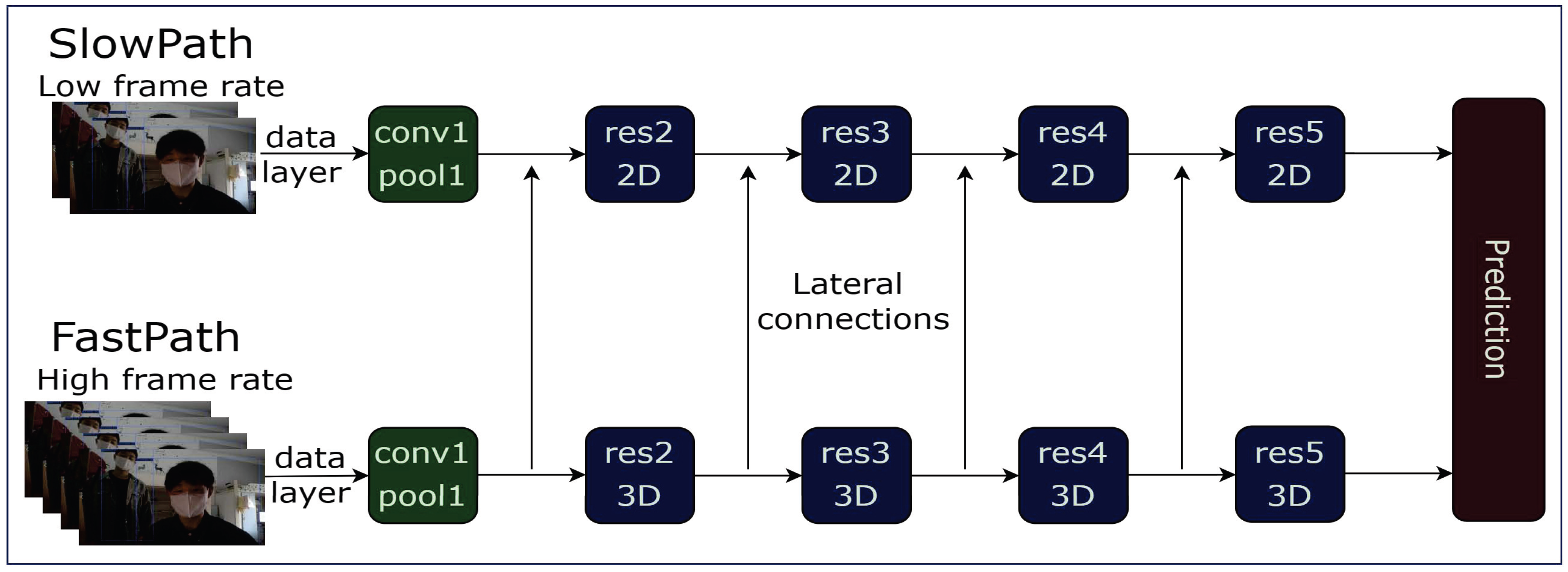
Figure 1. SlowFast flow chart, the upper layer is the slow channel to process spatial features, and the lower layer is the fast channel to obtain temporal features.
Electronics 11 03770 g001
Figure 2. SlowFast behavior analysis structure diagram. The detection results obtained by FasterRCNN, YOLOv3, YOLOX, or CascadeRCNN are fed to SlowFast to capture the action information.
Electronics 11 03770 g002
Figure 3. Schematic diagram of the RPN structure.
Electronics 11 03770 g003
Figure 4. Comparison of YOLOv3+SlowFast and FasterRCNN+SlowFast in the same frame image detection effect.
Electronics 11 03770 g004
Figure 5. Comparison of YOLOX+SlowFast, CascadeRCNN+SlowFast, and FasterRCNN+SlowFast in the same frame image detection effect.
Electronics 11 03770 g005
Table 1. Under VOC Dataset. Comparison of backbone networks, detection time delay, three IOU precision APs, and three object size precision APs.
MethodBackboneEvaluation TimeAP0.50–0.95AP50AP75APSAPMAPL
FasterRCNNResNet502.51 s0.5140.8100.5640.1020.3120.601
YOLOv3 (Ours)DarkNet531.92 s0.4860.7900.5370.1230.2820.586
Table 2. Under VOC Dataset. Comparison of AP50, Score-threshold, F1-score, Precision, Recall, and LAMR.
MethodAP50Score-ThresholdPrecisionRecallLAMRF1-Score
FasterRCNN0.81140.50.47020.91720.410.62
YOLOv3 (Ours)0.77890.50.76140.70500.460.73
Table 3. Based on YOLOX-S and VOC Dataset. Comparison chart of the accuracy of IOU, CIOU, EIOU and LIOU.
MethodAP0.50–0.95AP50AP75APSAPMAPL
IOU0.4490.6940.4930.1450.2870.510
CIOU0.4350.6940.4710.1270.2690.500
EIOU0.4540.7090.4950.1760.2970.515
LIOU(ours)0.4590.7170.5100.1740.3150.517
Table 4. Under COCO Dataset. Comparison of three IOU precision APs, and three object size precision APs.
MethodAP0.50–0.95AP50AP75APSAPMAPL
FasterRCNN0.3480.6270.3480.1820.4280.518
YOLOv3 (Ours)0.2330.5120.1820.0790.2600.429
YOLOX (Ours)0.3530.6540.3400.2030.4350.493
CascadeRCNN (Ours)0.3790.6280.3880.1820.4680.577
Table 5. Comparison of different algorithms for video frame detection latency and Spatio-temporal Action Detection time.
MethodHuman Detection TimeSpatio-Temporal Action Detection Time
FasterRCNN + SlowFast17 s12.5 s
YOLOv3 + SlowFast6.5 s5.7 s
YOLOX + SlowFast6.6 s7.9 s
CascadeRCNN + SlowFast16.6 s12.4 s
Publisher’s Note: MDPI stays neutral with regard to jurisdictional claims in published maps and institutional affiliations.