Fast 3D Liver Segmentation Using a Trained Deep Chan-Vese Model

Abstract

This paper introduces an approach for 3D organ segmentation that generalizes in multiple ways the Chan-Vese level set method. Chan-Vese is a segmentation method that simultaneously evolves a level set while fitting locally constant intensity models for the interior and exterior regions. First, its simple length-based regularization is replaced with a learned shape model based on a Fully Convolutional Network (FCN). We show how to train the FCN and introduce data augmentation methods to avoid overfitting. Second, two 3D variants of the method are introduced, one based on a 3D U-Net that makes global shape modifications and one based on a 3D FCN that makes local refinements. These two variants are integrated in a full 3D organ segmentation approach that is capable and efficient in dealing with the large size of the 3D volumes with minimal overfitting. Experiments on liver segmentation on a standard benchmark dataset show that the method obtains 3D segmentation results competitive with the state of the art while being very fast and having a small number of trainable parameters.

1. Introduction

Image segmentation and related tasks, such as object and scene segmentation, have a wide range of applications, including (but not limited to) content-based image retrieval, medical diagnosis, autonomous driving, object detection, face recognition, etc.

While image segmentation is a generic problem, object segmentation is the problem of delineating the boundary of a specific type of object, such as a dog in an image or a liver in a CT scan. This problem is very important for medical imaging where it is used for delineating tumors or other pathologies, estimating the volume of a heart, a liver or a swollen lymph node, etc. Even though radiologists have been handling the aforementioned medical imaging tasks, an increasing amount of research indicates that computer vision techniques have the potential to outperform radiologists in terms of speed and accuracy.

Generic image segmentation is usually a low-level task that finds the boundary of a region purely based on the intensity difference with the neighboring regions. Object segmentation is a high-level task that aims at finding the boundary of a specific object and uses the shape of the object to eliminate distractors and to project where the boundary should be in places where it is not visible.

The Chan-Vese method is a popular low level segmentation method that uses constant intensity models for the inside and outside regions and boundary length regularization to evolve a level set and find the minimum cost segmentation [1]. Its boundary length regularization is too simple and not capable of imposing specific object shape regularization for real applications such as object or organ segmentation.

For this reason, our recent work has generalized it as a Chan-Vese Neural Network (CVNN) to contain a more elaborate shape model based on a convolutional neural network (CNN), which is trained in a supervised way as a recurrent neural network (RNN) [2]. However, while the CVNN method showed promise outperforming the original Chan-Vese method, it did not show its full potential through real 2D object segmentation applications and comparisons with the state of the art methods in the field.

This paper takes the CVNN approach even further, bringing it to the level of the state of the art in 3D liver segmentation, with the following contributions:

-

It presents a generalization of the CVNN method [2] for 3D organ segmentation that employs a U-Net [3] for a better 3D shape model.

-

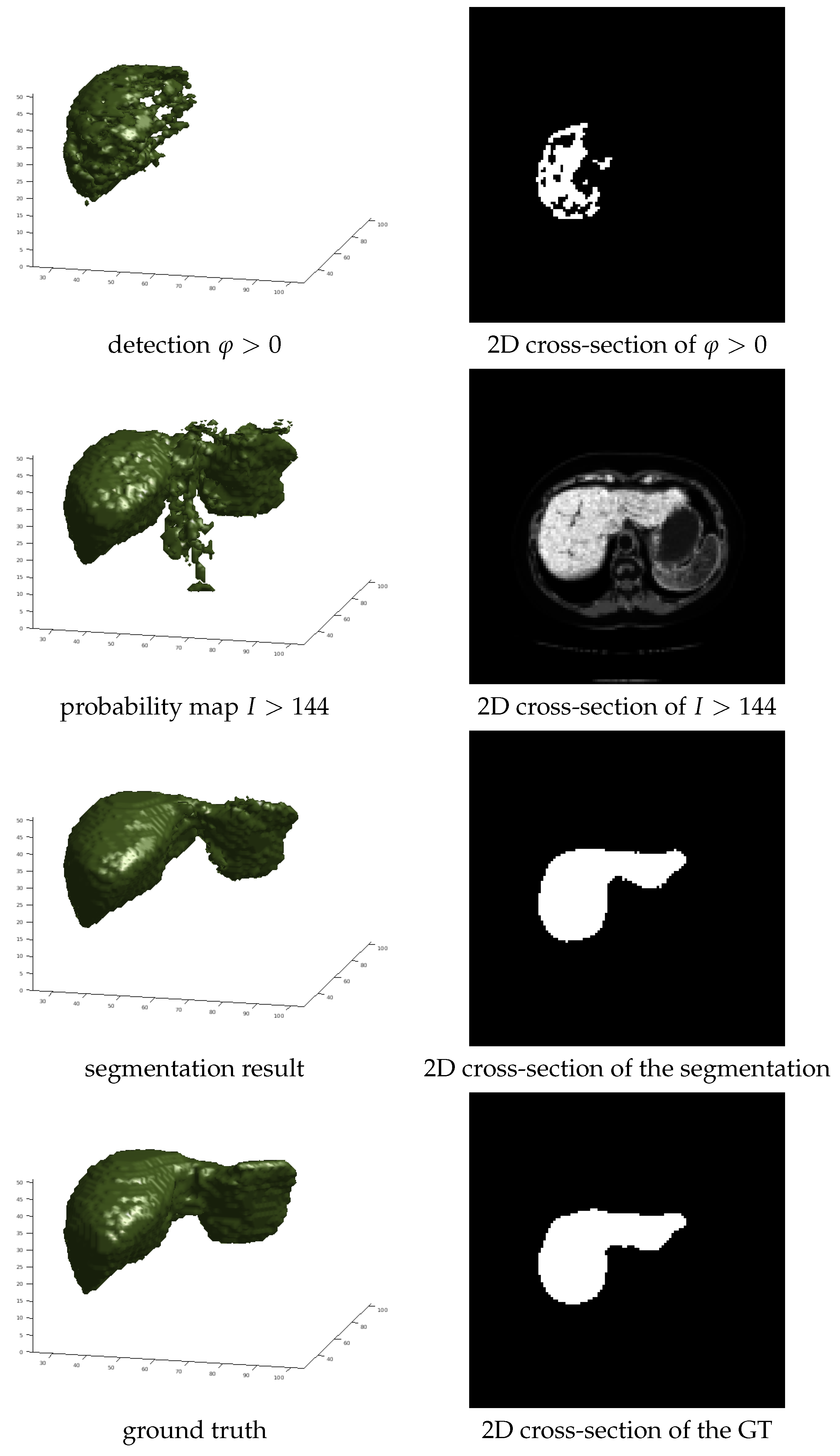
It shows how to improve the segmentation accuracy by employing liver probability maps as 3D CVNN-UNet data terms instead of the CT intensity. The probability maps and the initializations are obtained from the output of a pixel-wise organ detection algorithm.

-

It introduces novel types of perturbations based on connected components that induce variability in the initialization and help avoid overfitting, a problem that severely impacts the 3D CVNN-UNet accuracy even when using perturbations that are 3D extensions of [2].

-

It presents a full multi-resolution 3D liver segmentation application, where a computationally intensive 3D CVNN algorithm based on U-Net is used at low resolution, and a computationally efficient 3D CVNN algorithm is used to refine the low resolution result at the higher resolutions. The proposed method obtains results competitive with the state of the art liver segmentation methods.

Related Work

The U-Net has been extended to 3D segmentation tasks: 3D U-Net, which essentially replaces 2D convolutions with 3D convolutions; thus segments out 3D objects [4]. In principle, any variation of the 2D U-Net architectures [5,6] can be adapted for 3D tasks by using 3D convolutions instead. ComboNet combines 2D and 3D U-Net architectures in an end-to-end fashion where the 2D portion takes a full-resolution input and the 3D portion takes a resized input to reduce computation [7]. The outputs of the two sub-networks are combined with a series of convolution layers.

Because of state of the art results, researchers found different ways to enhance the U-Net, by introducing alterations to the architecture while maintaining the residual connections and its symmetric nature. For instance, the Attention U-Net added attention gating layers prior to each convolution block on the decoding part [5]. The authors claim that Attention-U-Net outperforms U-Net by around $2\%$; however, the ComboNet exemplified in their ablation study that the performance improvement achieved by the Attention U-Net might be case-specific, obtaining decreased performance compared to the U-Net [7].

Another state of the art U-Net variation is U-Net++ [6]. It replaces the residual connections with a series of nested residual connections and provides a $2\%$ improvement in accuracy while increasing the number of parameters by around $20\%$. In principle, the encoding part of the U-Net can be replaced by classification architectures without the fully connected layer(s) of the classification models. For instance UResNet [8] combines the state of the art ResNet [9] architecture with the U-Net architecture. Another recent U-Net-based method is ObeliskNet [10]. It learns spatial filters and filter offsets in an end-to-end manner, obtaining a sparse model with few parameters.

One of the many recent examples of U-Net-based methods is nnU-Net [11]. It uses a 3D U-Net architecture with slight modifications and tailored training, as well as data augmentation and post-processing methods to obtain state of the art results. The authors of the nnU-Net also proposed modifications to the U-Net architecture itself but the ablation study showed no significant improvement from the architectural changes.

The latest organ segmentation works use transformers as part of the U-Net to obtain state of the art segmentation performance. Transformers are attention-based models that have obtained state of the art results in many applications, from natural language processing to image classification and object detection [12,13,14]. For organ segmentation, SETR and UNETR replace the encoder part of the U-Net with a vision transformer [15,16]. CoTr places the vision transformer between the encoder and decoder parts of the U-Net [17]. Any of these developments could be used to replace the 3D UNet from our model to further boost the segmentation of the method.

One of the issues with the deep learning methods is that they need a large number of manually labeled images, which are almost always scarce in the medical imaging domain. Furthermore, annotations, especially segmentations, are not $100\%$ accurate, and the data are noisy. Although deep learning is known to handle noise well, it is not immune to overfitting. Once the lack of annotated data is taken into consideration, overfitting becomes a more significant issue. Often, researchers exercise different techniques to avoid overfitting, such as data augmentation and early stopping. Thus, in order to maintain a state of the art accuracy with a small data set, and with a relatively small number of parameters and computations, researchers are combining neural networks with level sets.

An approach that combined NN with level sets to segment out the left ventricle of the heart from cardiac cine magnetic resonance (MR) images was proposed in [18]. They used Deep Belief Networks (DBN) [19] as a region of interest (ROI) detector, which mainly yields a rectangle bounding box that encloses the object of interest. Then, within the ROI, Otsu’s gray-scale histogram-based thresholding [20] is used to obtain an initial segmentation. The segmentation derived at this stage is used as a shape prior and/or initialization for the next stage. Then, Otsu’s segmentation is fed into a distance regularized level set formulation, which eventually yields the final segmentation [21].

Some recent works merge level sets with deep learning [22,23]. Level sets are combined with VGG16 [24] to segment out salient objects in [22]. The level set formulation of active contours is used along with the optical flow for the task of moving object segmentation in [23]. Also, to segment out lung nodules, machine learning regression models are used in conjunction with level sets to obtain a better curve evolution velocity model at a given point in [25].

LevelSet R-CNN modified the Mask R-CNN [26] architecture such that it has 3 additional mask heads, of which one predicts a truncated signed distance transform, the other predicts Chan-Vese features and the last predicts the Chan-Vese hyper parameters [27].

The Deep Implicit Statistical Shape Model (DISSM) method uses implicit shape models based on deep learning with an iterative refinement also based on deep learning, to segment out certain organs in 3D CT scans [28]. The method does not necessarily reduce the computation cost, yet it definitely improves the segmentation quality.

A hybrid active contour and UNet architecture was designed to segment out breast tumors in [29]. The method takes in radiologist annotation as initialization, while in our case we use a detection algorithm to provide the initialization.

Our method differs from all these level set formulations. First, unlike [18], we are using a U-Net CNN instead of a DBN, and the U-Net is used as the shape model instead of distance or length-based regularization, and we are not using Otsu’s thresholding. One study [25] uses a least-squares-based regression method to model velocity; we are using the CNN to replace the curvature term in an Euler-Lagrange equation. The researchers in [22] use VGG16 as a backbone to compute the initialization along with upsampling and refining the upsampled level sets. Moreover, they use a level set function as a loss function that is minimized. In contrast, our formulation uses the level set produced by the CNN as a shape model instead of length-based regularization and combines it with the Chan-Vese intensity-based update to obtain a model with very few parameters. In their next paper, [23] minimize a Euler-Lagrange equation based on level sets produced by ResNet101 [9], and unlike us, their formulation does not use the output of the CNN to replace the curvature. They only use it to estimate the Heaviside and subsequent average intensity. The LevelSet R-CNN [27,29] use the CNN model to learn almost every single parameter in the Chan-Vese and active contour formulation respectively, whereas we estimate those hyper-parameters algebraically. The VGG16, ResNet101, Mask R-CNN are all very computationally intensive; in comparison, our CNN is very efficient in terms of computation complexity and small in terms of number of parameters. Last but not least, our model is an RNN (Recurrent Neural network); we iterate over the same input to improve the result, whereas none of the aforementioned algorithms use an RNN. However, we must mention that [23] works iteratively from one frame to the next, i.e., the segmentation of frame at time t is used as initialization for time $t+1$.

In this paper we show how to use the U-Net model as part of the Chan-Vese NN framework (see Section 2.3.1), to obtain state of the art 3D segmentation results with 140+ times fewer parameters than the original U-Net. In principle most of the above methods could be used as part of our method to further improve results.

Chan-Vese Overview

The Chan-Vese Active contour [1] is aimed at minimizing the Mumford-Shah energy [30]:

$$E\left(C\right)={\int }_{C_i}{(I\left(u\right)-{\mu }_i)}^{2}du+{\int }_{C_o}{(I\left(u\right)-{\mu }_o)}^{2}du+\nu \left|C\right|$$

(1)

where I denotes the image intensity, C is the curve to be fitted, $C_i$, $C_o$ are the regions inside and outside the curve C, respectively, and ${\mu }_i$ and ${\mu }_o$ are the intensity averages of image I inside and outside the curve C, respectively.

The Chan-Vese method takes a level set approach where the curve C is represented as the 0—level set of a surface $\phi$, i.e., $C=\left\{\right(x,y\left)\right|\phi (x,y)=0\}$. Usually $\phi (x,y)$ is initialized as the signed Euclidean distance transform of C, i.e., $\phi >0$ inside the curve C and $\phi <0$ outside, and the magnitude of $\phi (x,y)$ is the distance of the point $(x,y)$ to the closest point on curve C. Then the energy (1) is extended to an energy of the level set function $\phi$:

$$E\left(\phi \right)=\int {(I\left(u\right)-{\mu }_o)}^2(1-H_{ϵ}\left(\phi \left(u\right)\right))du+\int {(I\left(u\right)-{\mu }_i)}^2{H}_{ϵ}\left(\phi \left(u\right)\right)du+\nu \int {\delta }_{ϵ}\left(\phi \left(u\right)\right)|\nabla \phi \left(u\right)|du$$

(2)

where $H_{ϵ}$ is the smoothed Heaviside function

$$H_{ϵ}\left(z\right)=\left\{\begin{array}{cc}0\hfill & \mathrm{if}z<-ϵ\hfill \\ 1\hfill & \mathrm{if}z>ϵ\hfill \\ \frac{1}{2}[1+\frac{z}{ϵ}+\frac{1}{\pi }sin\left(\frac{\pi z}{ϵ}\right)]\hfill & \mathrm{if}\left|z\right|<ϵ\hfill \end{array}\right.$$

(3)

and ${\delta }_{ϵ}$ is its derivative. The parameter $\nu$ controls the curve length regularization $\int |\nabla \phi |$. When $\nu$ is small, the curve (segmentation) C will have many small regions while when $\nu$ is large, the curve C will be smooth and the segmented regions will be large.

The energy is minimized alternatively by updating ${\mu }_i,{\mu }_o$

$$\begin{array}{cc}\hfill {\mu }_i^t=& \frac{\int I\left(u\right)H_{ϵ}\left({\phi }^t\left(u\right)\right)du}{\int H_{ϵ}\left({\phi }^t\left(u\right)\right)du}\hfill \\ \hfill {\mu }_o^t=& \frac{\int I\left(u\right)[1-H_{ϵ}\left({\phi }^t\left(u\right)\right)]du}{\int [1-H_{ϵ}\left({\phi }^t\left(u\right)\right)]du}\hfill \end{array}$$

(4)

then updating $\phi$:

$${\phi }^{t+1}={\phi }^t+\eta [\kappa \left({\phi }^t\right)+{(I-{\mu }_o^t)}^2-{(I-{\mu }_i^t)}^2]$$

(5)

where $\kappa \left(\phi \right)=\nu \mathrm{div}\frac{\nabla \phi }{|\nabla \phi |}$.

2. Proposed Method

The Chan-Vese neural network (CVNN) [2] generalizes the update Equation (5) by replacing the divergence term $\kappa \left(\phi \right)=\nu \mathrm{div}\frac{\nabla \phi }{|\nabla \phi |}$ responsible for length regularization with a Convolutional Neural Network (CNN) $g(\phi ,\beta )$:

$${\phi }^{t+1}={\phi }^t+\eta [g({\phi }^t,\beta )+{(I-{\mu }_o^t)}^2-{(I-{\mu }_i^t)}^2]$$

(6)

The iterative update (6), makes the algorithm behave as a Recurrent Neural Network that takes a preset number of steps T. It is illustrated in Figure 1.

We can see that at each iteration the model takes ${\phi }^t$ as input and passes it through the CNN portion of the model $g({\phi }^t,\beta )$, which imposes the shape information. The CNN output is then passed to the Chan-Vese update (6), along with average image intensity values ${\mu }_i^t,{\mu }_o^t$ (from Equation (4)) inside and outside of the implicit 3D surface ${\phi }^t\left(x\right)=0$. This way ${\phi }^{t+1}$ is obtained and is fed back into the next iteration of the RNN. After T iterations, ${\phi }^T$ is thresholded to obtain the segmentation result.

Training. Training is conducted using backpropagation through time,

$$\frac{\partial L}{\partial \beta }=\frac{\partial L}{\partial {\phi }^T}·\eta ·\sum _{k=1}^T\{\frac{\partial g({\phi }^{k-1},\beta )}{\partial \beta }·\prod _{t=k}^{T-1}\frac{\partial {\phi }^{t+1}}{\partial {\phi }^t}\},$$

(7)

where

$$\frac{\partial {\phi }^{t+1}}{\partial {\phi }^t}=1+\eta \left(\frac{\partial g({\phi }^t,\beta )}{\partial {\phi }^t}-2(I-{\mu }_o)·\frac{\partial {\mu }_o\left({\phi }^t\right)}{\partial {\phi }^t}+2(I-{\mu }_i)·\frac{\partial {\mu }_i\left({\phi }^t\right)}{\partial {\phi }^t}\right),$$

(8)

and

$$\begin{array}{cc}\hfill \frac{\partial {\mu }_i\left({\phi }^t\right)}{\partial {\phi }^t}& =\frac{{\delta }_{ϵ}\left({\phi }^t\right)·(I-{\mu }_i)}{\int H_{ϵ}\left({\phi }^t\left(x\right)\right)dx},\hfill \\ \hfill \frac{\partial {\mu }_o\left({\phi }^t\right)}{\partial {\phi }^t}& =\frac{{\delta }_{ϵ}\left({\phi }^t\right)·({\mu }_o-I)}{\int (1-H_{ϵ}\left({\phi }^t\left(x\right)\right))dx},\hfill \end{array}$$

(9)

and where $H_{ϵ}$ has been defined in Equation (3) and ${\delta }_{ϵ}$ is its derivative.

The CVNN update Equation (6) depends on the input image I and the initialization ${\phi }^0$. In order for the CVNN model to work well, the image I should satisfy the assumption that the intensity inside and outside the object of interest are relatively constant. A standard CT image does not meet the constant intensity assumption outside the object, because the CT intensities outside an organ have a large range of values from very low (e.g., air) to very high (e.g., bone).

For these reasons we will introduce methods to construct voxelwise probability maps for the organ of interest, with high values inside the organ and low values outside, thus better satisfying the intensity assumptions and hence better suited as input for CVNN.

The other CVNN input is the initialization ${\phi }^0$, which will be obtained using a pixelwise detection algorithm, and this initial detection will also be used to construct the probability map.

The whole organ segmentation algorithm is summarized in Algorithm 1 and illustrated in Figure 2.

Here $\delta \left(s\right)$ is 1 if statement s is true, otherwise 0, and $DT$ is the 3D distance transform. A number of $T=4$ iterations have been used for the 3D CVNN-UNet experiments.

Algorithm 1 Deep Chan-Vese 3D Organ Segmentation

Input: CT scan C. Output: Segmentation map S. 1: Resize raw input C to isotropic low and medium resolution maps $C_L$, $C_M$. 2: Compute pixelwise detection map D (Section 2.1) 3: Compute probability map I from $C_L$ and $\delta (D>0)$ (Section 2.1) 4: Run 3D CVNN-UNet with input I and ${\phi }^0=DT(D>0)$, obtaining ${\phi }^T$ (Section 2.3.1) 5: Resize ${\phi }^T$ to medium resolution using trilinear or tricubic interpolation, denote it as $\phi$ 6: Compute probability map I from $C_M$ and $\delta (\phi >0.5)$ 7: Run 3D CVNN with input I and ${\phi }^0=DT(\phi >0.5)$, obtaining ${\phi }^1$ (Section 2.3.2) 8: Obtain segmentation map $S=\delta ({\phi }^1>0)$

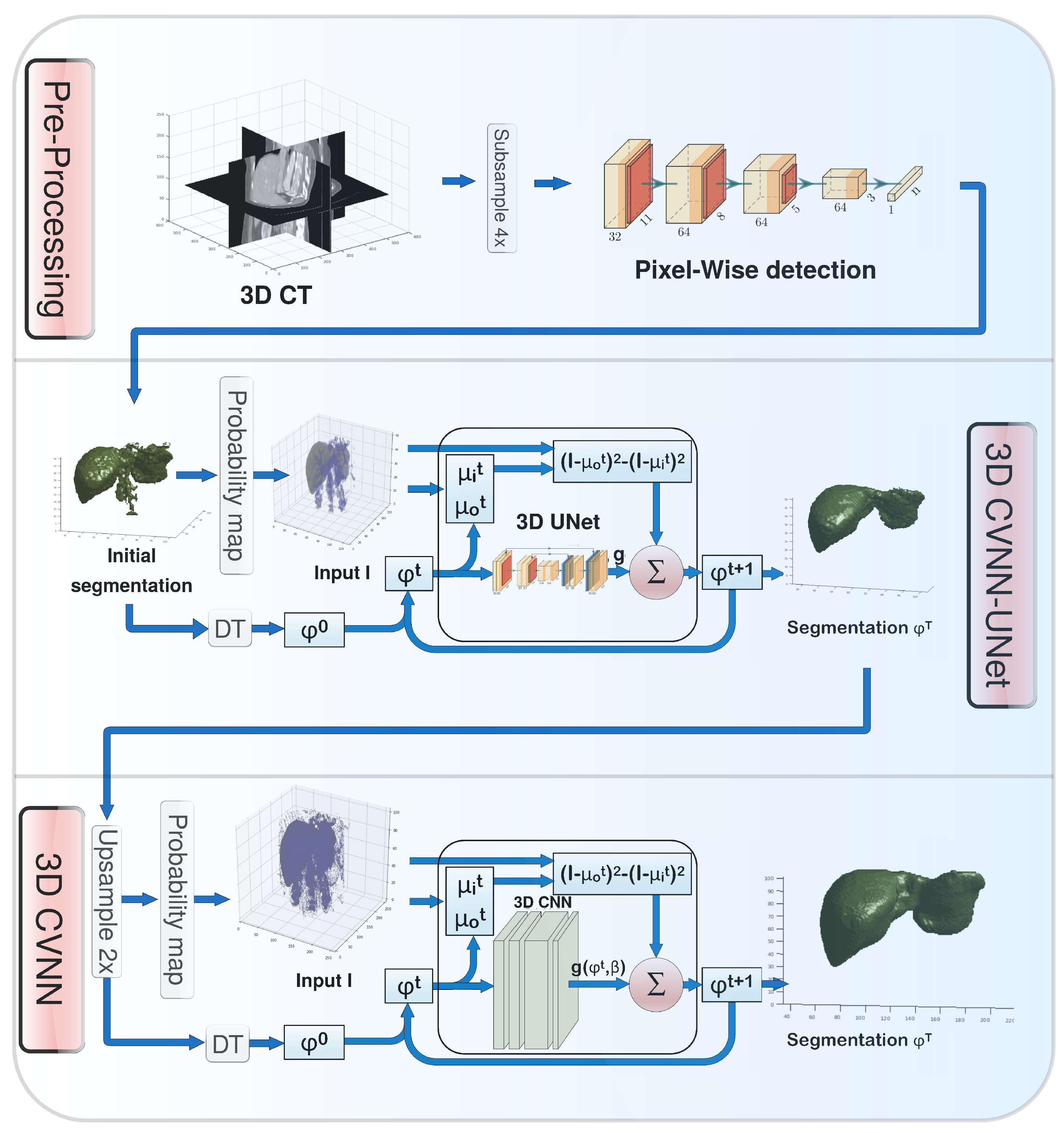
2.1. Pre-Processing

The Chan-Vese algorithm is a local algorithm, and so is CVNN, meaning that one should start with a proper initialization for these models to perform well. The following CNN detection algorithm described below has been used for initialization.

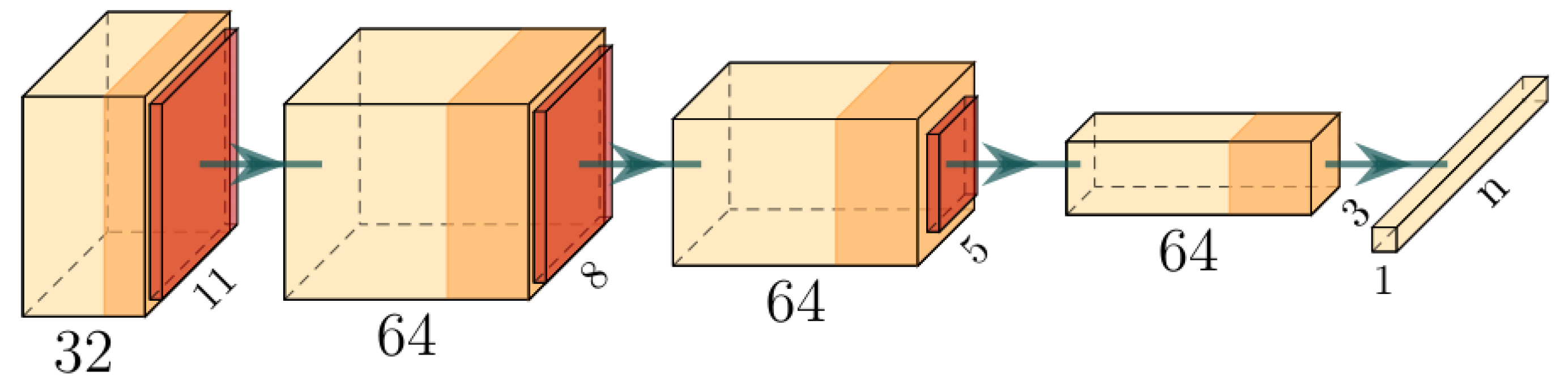
2.1.1. Pixelwise Organ Detection

A 2D CNN was trained for the purpose of classifying each CT voxel whether it is inside an organ or not, working on the axial CT slices at $128\times 128$ resolution. This detection algorithm obtains coarse organ segmentations D, which will be used to generate organ probability maps. These coarse organ segmentations are also used to obtain the initializations ${\phi }^0$ for Equation (6) using the 3D distance transform.

The CNN consists of 4 convolution layers with $3\times 3$ kernels, as illustrated in Figure 3.

All the convolution layers have 64 filters except the first layer, which has 32 filters, and the last layer has n filters, where n represents the number of classes or more specifically in our case, the number of organs, $n-1$, and background to be detected. In our experiments we used $n=15$ classes because using a larger number of classes reduced false positives.

The first 3 convolution layers are followed by ReLU and max-pooling with stride 1. All the convolution layers have stride 1 and no padding, so that during training, the network takes input patches of size of $11\times 11$ and yields an output of $1\times 1\times n$, which is then passed through a softmax layer.

Training. Organs do vary in size, which creates a severe class imbalance. In order to handle this issue, the outputs of the last activation are then fed into a weighted Binary Cross-Entropy (BCE) (10) [3] loss function, where careful consideration is needed while choosing the weights,

$$L=-\frac{1}{n}\sum _{i=1}^n{\alpha }_i{Y}_{i}ln\widehat{R_i}-(1-{\alpha }_i)(1-Y_i)ln(1-\widehat{R_i})$$

(10)

where ${\alpha }_i$ is the weight for the i-th class, $Y_i\in \{0,1\}$ is the ground truth of that class, and $\widehat{R_i}$ is the corresponding prediction for that class, i.e., $\widehat{R_i}\in [0,1]$.

An initial approach for choosing the class weights would be ${\alpha }_i=\frac{1}{N_i}$ where $N_i$ is the number of samples from the i-th class. This approach is mostly fine when training is conducted with all the samples or sub-sampled at the same rate across all classes. It becomes, however, less effective when samples of different classes are subsampled at different rates. For instance, in our case, the background samples were subsampled at a lower rate than any positive samples for organs, as most of a CT scan is background. To account for subsampling, the weights are changed as ${\alpha }_i=\frac{1}{\widehat{N_i}}$ where $\widehat{N_i}=s_i·N_i$ is number of expected samples from the i-th class. Here $s_i$ is the subsampling ratio for the i-th class.

Inference. During inference, the detection algorithm can take in any input of size $k\times m$, with $k,m\ge 11$. In that case the output of the detection algorithm would be $(k-10)\times (m-10)\times n$, where n is again number of detected classes, including the background. For convenience, one can pad the output of each detection map with zeros to reach size $k\times m\times n$, so that the axial dimension of the output is the same as the input.

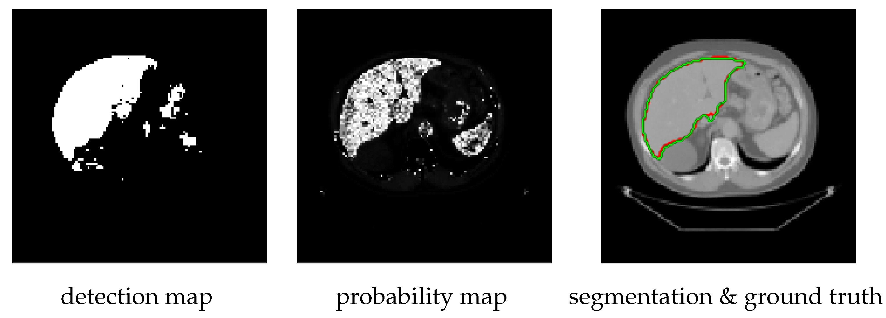
2.1.2. Constructing Probability Maps

The probability map gives a measure of how likely each pixel, based on its intensity, is inside the object of interest. As opposed to the detection map which obtains only a rough segmentation, the probability map follows the organ boundaries very closely, at the cost of a noisy appearance inside the organ. An example of a detection map and probability map is shown in Figure 4. The probability map computation is described in detail in Algorithm 2.

Algorithm 2 Probability Map Computation

Input: CT scan C, initial binary mask D, number of bins $N^{bins}$. Output: Probability map I. 1: Extract pixels inside the mask $\mathbf{u}=C(D>0)$ 2: Construct $N^{bins}$ equally spaced $bins$ in the range $[min(\mathbf{u}),max(\mathbf{u}\left)\right]$ 3: Compute counts $\mathbf{n}=histogram(\mathbf{u},bins)$ 4: Obtain $I\left(x\right)=\mathbf{n}\left(C\right(x\left)\right)/max\left(\mathbf{n}\right)$

Here C is the actual CT scan and $I\in [0,1]$ is the obtained probability map that will be used in Equation (6). Optionally the probability map range can be scaled by 255 for convenience. In our application we used $N^{bins}=16$.

2.2. 2D Approach

To evaluate the benefit of using a 3D approach, we have also experimented with 2D approaches that use two main ways to replace $g({\phi }^t,\beta )$ in (6) with: (i) a shallow CNN called 2D CVNN described in Section 2.2.1 (ii) a U-Net variant called 2D CVNN-UNet described in Section 2.2.2. Before we dive into architecture details we would like to lay out the preprocessing steps that are specific to 2D inputs at this stage.

Multiple Initializations. In order to improve model generalization, various initializations were used for each input image I during training. In fact, rarely the same initialization was used twice during training. The initialization was selected at random from the following: $10\%$ of the time the initialization was obtained the same way as it is obtained at test time through the detection map, which is a rough initial CNN segmentation. A total of $30\%$ and the remaining $60\%$ of the time the initializations were obtained from the same detection map and the ground truth Y, respectively, by the following distortions: first, semicircles with a random radius were added, or holes were punched at random locations on the boundary of the detection map or Y, then Gaussian noise was added to the distorted map around the edge. This process is illustrated in Figure 5.

By varying the number of different initializations of the same image, we observed that more initializations resulted in better generalization.

The architectures of the two 2D approaches, 2D CVNN and 2D CVNN-UNet, are described next.

2.2.1. 2D CVNN Architecture

The CNN part has a convolution layer with one convolutional filter of size $3\times 3$, two convolutional layers with 3 filters of size $3\times 3$ with padding, followed by a convolutional layer with 3 filters of size $1\times 1$ followed by exponential linear unit (ELU), instead of ReLU activation, and finally another convolutional layer with one filter of size $1\times 1$. The $3\times 3$ filters used padding such that the size of the output was kept the same as the size of the input. This network has 214 trainable parameters.

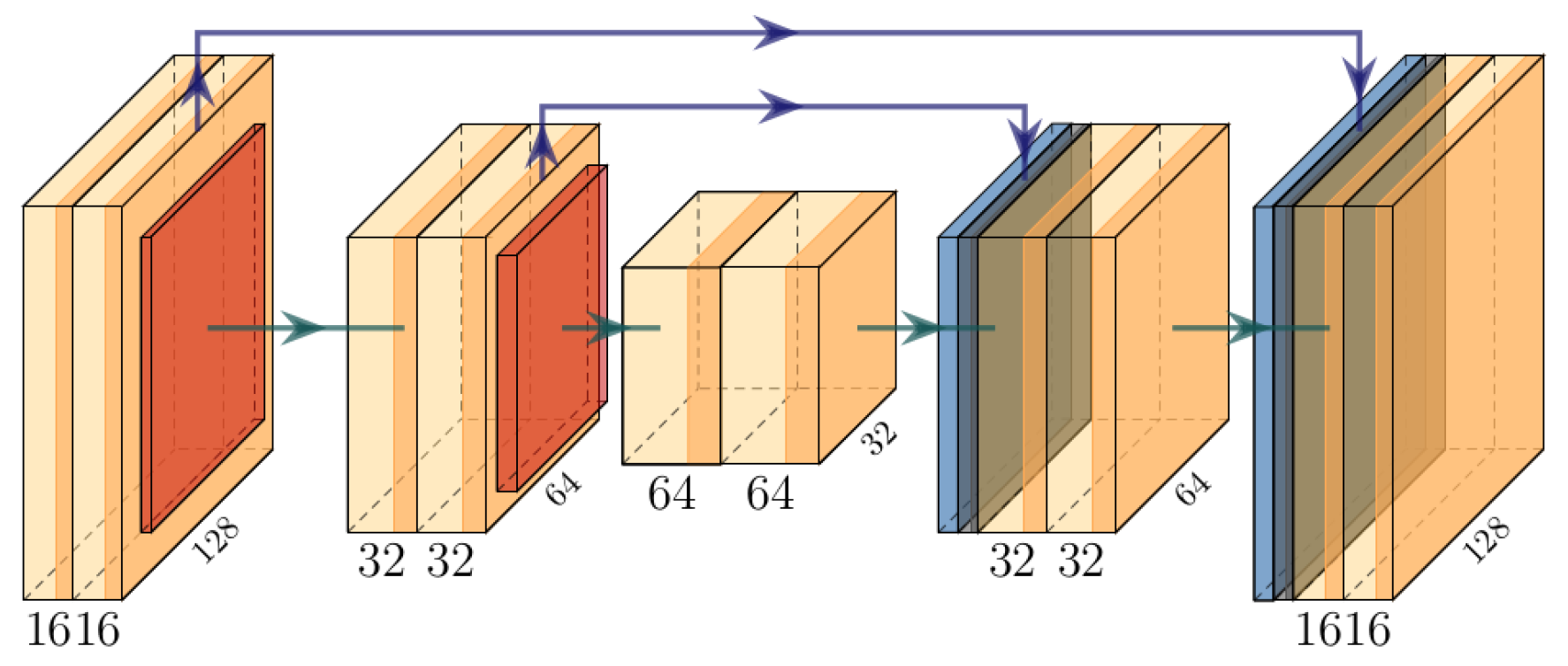
2.2.2. 2D CVNN-UNet

A 2D U-Net was used with 2 convolution blocks in both the encoding and decoding paths of the U-Net, and each convolution block has 2 convolution layers. Each convolution layer is followed by an exponential linear unit (ELU) activation. As illustrated in Figure 6, each layer of the first block has 16 filters which double after each maxpooling, and halve after each upsampling, in a similar way to the regular U-Net. Each filter is of size $3\times 3$. With these aforementioned configurations this network architecture has only 147,473 trainable parameters in contrast to a standard U-Net with about 50 million parameters.

2.3. 3D Approach

As pointed out in Section 2.2.2, the CVNN is not capable of reaching the desired solution when the initialization is far away from the ground truth. For the 3D approach, we address this problem using a 3D CVNN-UNet that is capable of obtaining a high-level representation and is therefore more likely to find the solution independent of initialization. However, because the 3D U-Net uses large amounts of data, we are constrained to use a low resolution input in this case. A 3D CVNN on higher resolution data is then used to refine the output of the 3D CVNN-UNet and obtain the final result.

These two architectures will be described next. The 3D approach that uses both the low resolution 3D CVNN-UNet and the higher resolution 3D CVNN is the Deep Chan-Vese 3D method described in Algorithm 1.

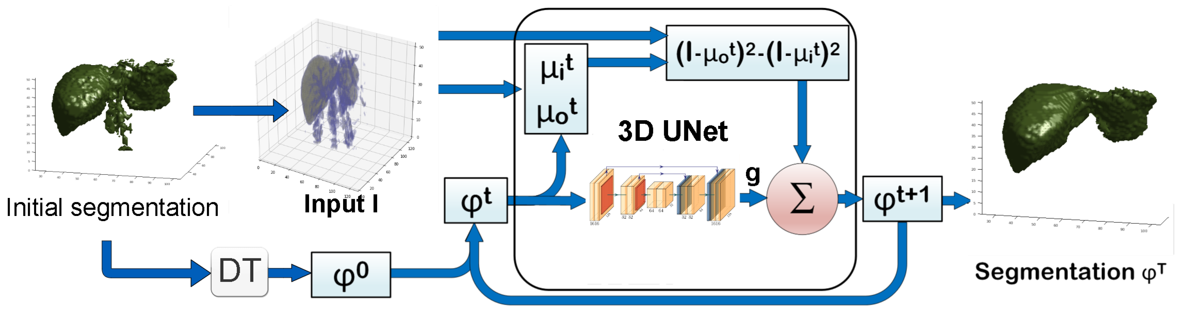
2.3.1. 3D CVNN-UNet with Low-Resolution Input

Due to GPU memory limitations, the 3D CVNN-UNet is applied to low-resolution inputs. More exactly, if the original data size is $512\times 512\times 4k$ for the largest possible integer k, the 3D CVNN-UNet input is resized to $128\times 128\times k$, and so are the detection and probability maps. This way, the input is small enough to be able to fit multiple volumes in the GPU memory with the 3D CVNN-UNet architecture.

Overall, to go from CVNN to 3D CVNN-UNet, the CNN portion of the original CVNN algorithm is replaced by a 3D U-Net, and the Chan-Vese update (6) takes place in 3D, not in 2D.

The same architecture configuration for the UNet portion of the 3D CVNN-UNet is used as in Section 2.2.2. The only difference is the convolution layers are 3D, i.e., the kernels are $3\times 3\times 3$. An example of the detection map, thresholded probability map, segmentation result by the 3D CVNN-UNet and ground truth is shown in Figure 7.

2.3.2. 3D CVNN with Medium-Resolution Input

The 3D CVNN-UNet obtains segmentations that are relatively close to the ground truth, however they have a low resolution. The segmentation maps obtained by the 4-iteration 3D CVNN-UNet are upsampled from $128\times 128\times k$ to $256\times 256\times 2k$. These upsampled segmentations are used as new detection maps, and probability maps are computed using Algorithm 2.

There are three main purposes for this step:

1.

To further improve the accuracy given the new detection and probability maps.

2.

To obtain finer medium resolution segmentations, since the low-resolution segmentation would look coarse when upsampled.

3.

To show that by combining the 3D CVNN-UNet and the 3D CVNN, one can achieve high accuracy for medium resolution input with a reduced computation complexity.

The 3D CVNN has three convolution layers with 3 filters of size $3\times 3\times 3$ with padding, followed by a convolutional layer with 3 filters of size $1\times 1\times 1$, followed by exponential linear unit (ELU) activation, and finally another convolutional layer with 1 filter of size $1\times 1\times 1$. The $3\times 3\times 3$ filters use padding to have the output size equal to the input size, so that the Chan-Vese update (6) can be computed for the entire volume at once.

2.4. Implementation Details

All models have been implemented in PyTorch [31] with CUDA, where new layers have been constructed for the computation of ${\mu }_i,{\mu }_o$ and for the Chan-Vese update (6).

Training details. Training is conducted using triplets $(I_i,Y_i,D_i)$ containing the full input 3D images $I_i$ (at the desired resolution) with their corresponding desired segmentation maps $Y_i$ and initialization binary maps $D_i$. The initial level set volume ${\phi }^0$ was obtained from each binary map $D_i$ as the signed 3D distance transform.

Recurrent Neural Networks (RNN) are more affected by vanishing and exploding gradients than feed-forward CNNs. Such is the case for the CVNN, which is an RNN, and therefore gradient clipping and regularization need to be used. However, a better and more stable solution was obtained using the Combo loss [32], which is a weighted combination of the weighted Binary Cross-Entropy (BCE) loss [3] and Dice loss [33]. By using this loss, not only does one not need to worry about exploding gradients, but the Combo loss authors also point out it promises better generalization. The Combo loss can be formulated as

$$L\left(\mathsf{\beta }\right)=({\alpha }_1-1)\frac{{\sum }_{i=1}^N{Y}_i\widehat{R_i}+s}{{\sum }_{i=1}^N{Y}_i+{\sum }_{i=1}^N\widehat{R_i}+s}-\frac{{\alpha }_1}{N}\sum _{i=1}^N{\alpha }_2{Y}_{i}ln\widehat{R_i}-(1-{\alpha }_2)(1-Y_i)ln(1-\widehat{R_i}),$$

(11)

where s is a small positive smoothing factor, $\mathsf{\beta }$ are the U-Net weights, $\widehat{R_i}\in [0,1]$ is the prediction for voxel i after sigmoid normalization, and ${\alpha }_1,{\alpha }_2\in [0,1]$ are tuning parameters, fixed as ${\alpha }_1=0.7$ and ${\alpha }_2=0.5$ in this paper.

When the number of iterations T is large, the loss (11) could have many local optima. To avoid getting stuck in a shallow optimum, we used the result of a trained RNN with fewer iterations as initialization, similar to [34]. We therefore started with training a 1-iteration 3D CVNN, then used it as initialization for the 2-iteration one, and so on.

To be able to better handle local minima, we dynamically changed the learning rate using an enlarged cosine wave, which is a modification of the [35] cosine annealing wave,

$${\alpha }_i=\frac{{\alpha }_1}{2}{\beta }^{⌊\frac{i·r}{n}⌋}\left(cos\left(\frac{\pi mod(i-1,n/r)}{n-⌊\frac{i·r}{n}⌋}\right)+1\right),$$

(12)

where ${\alpha }_i$ is the learning rate for the $i^{th}$ epoch, ${\alpha }_1$ is the largest possible learning rate for which the gradient does not explode, $\beta$ is an augmentation factor for which we took $\beta =1$, and n and r are the number of epochs to be run and number of waves, respectively.

Multiple Initializations. For better generalization, the CVNN is trained with various initializations for each input image I. In fact, we rarely fed the same initialization twice during the training. There are two main types of initializations:

1.

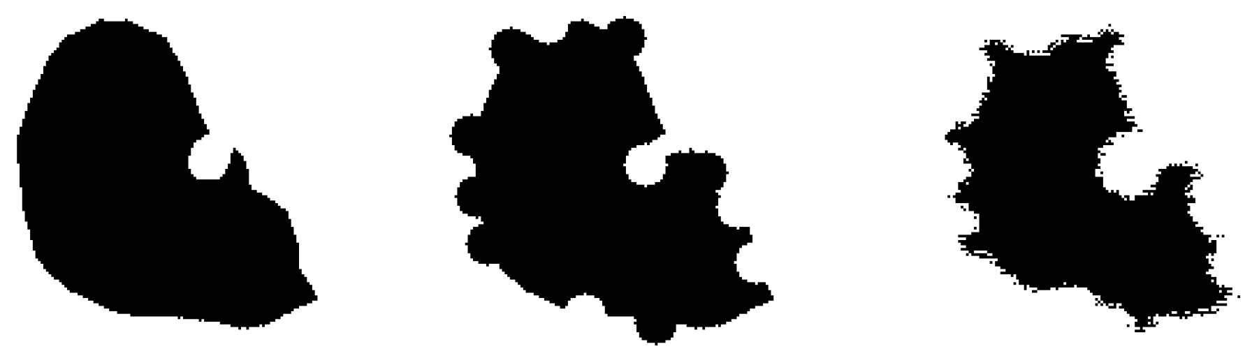
Thresholding the probability map $I>t$ with a random threshold t. For the 3D CVNN-UNet, t is randomly chosen from $\{64,80,96\}$. These values could range a larger span but for this work these values were enough to sustain generality. Then $25\%$ of the smallest connected components of the thresholded probability map are deleted at random. Those values are picked so that the Dice coefficient of $I>t$ for each t and the Dice of the detection map $D>0$ have roughly the same value, yet each initialization would have different false positives and false negatives. This would help train the CVNN to recover the correct shape from many scenarios and thus improve generalization. It is similar to having a golf player practice hitting the hole in 4 shots from a large number of locations roughly at the same distance from the hole.

2.

When we do not use the above connected component-based initialization, for $50\%$ of the time, the initialization was obtained the same way as at test time, namely through the detection map $D>0$. Another $20\%$ and the remaining $30\%$ of the time, the initializations were obtained from the detection map and ground truth Y, respectively, by the following distortions: first, semi-spheres with a random radius were added, or holes were punched at random locations on the boundary of the detection map or Y, then Gaussian noise was added to the distorted map around the boundary.

We trained with various numbers of different initializations of the same image and observed that more initializations resulted in better generalization.

3. Experiments

Experiments are performed for liver segmentation with four fold cross-validation on a standard multi-organ segmentation dataset [36].

3.1. Data

The multi-organ segmentation dataset [36] contains 90 CT scans, of which 43 are from the TCIA Pancreas-CT dataset [37,38,39] and 47 from the BTCV dataset [40,41]. Gibson et al. [36] reviewed and improved the existing organ segmentations from the corresponding datasets and provided segmentations for those that did not exist.

The pixel values of the original CT are preprocessed by Algorithm 3 so that the input C is in the range $[0,255]$.   

Algorithm 3 Input preprocessing

Input and Output: CT scan C. 1: Lower bound $C[C<-350]=-350$ 2: Upper bound $C[C>350]=350$ 3: Shift and scale $C=(C+350)·255/700$

The CT scans have been interpolated to make them isotropic (have the same resolution in all three directions), with axial dimensions of $512\times 512$. Then the isotropic CT scans were resized to low and medium resolution: if the isotropic input is $512\times 4k$ then the medium resolution is $256\times 256\times 2k$ and the low resolution is $128\times 128\times k$.

3.2. Metrics

Given a segmentation S and the annotation Y of a volume, we will evaluate the Dice coefficient $2|S\cap Y|/\left(\right|S|+|Y\left|\right)$, the symmetric mean boundary distance defined as $(\overline{D(S,Y)}+\overline{D(Y,S)})/2$ and the symmetric 95% Hausdorff distance $(P_{95}\left(D(S,Y)\right)+P_{95}\left(D(Y,S)\right))/2$. Here $D(S,Y)$ is the set of distances from the boundary pixels of S to the nearest boundary pixels of Y, and $P_{95}\left(X\right)$ is the 95 percentile of X. These metrics have also been used in [36].

We have observed that the detection algorithms from Section 2.1.1 did not seem to generalize as well on the BTCV dataset as the Pancreas-CT dataset [39]. There are two factors that might affect detection and segmentation performance for the BTCV dataset: the CT scans are not contrast-enhanced, and some of the patients have metastatic liver cancer, unlike in the TCIA Pancreas-CT dataset.

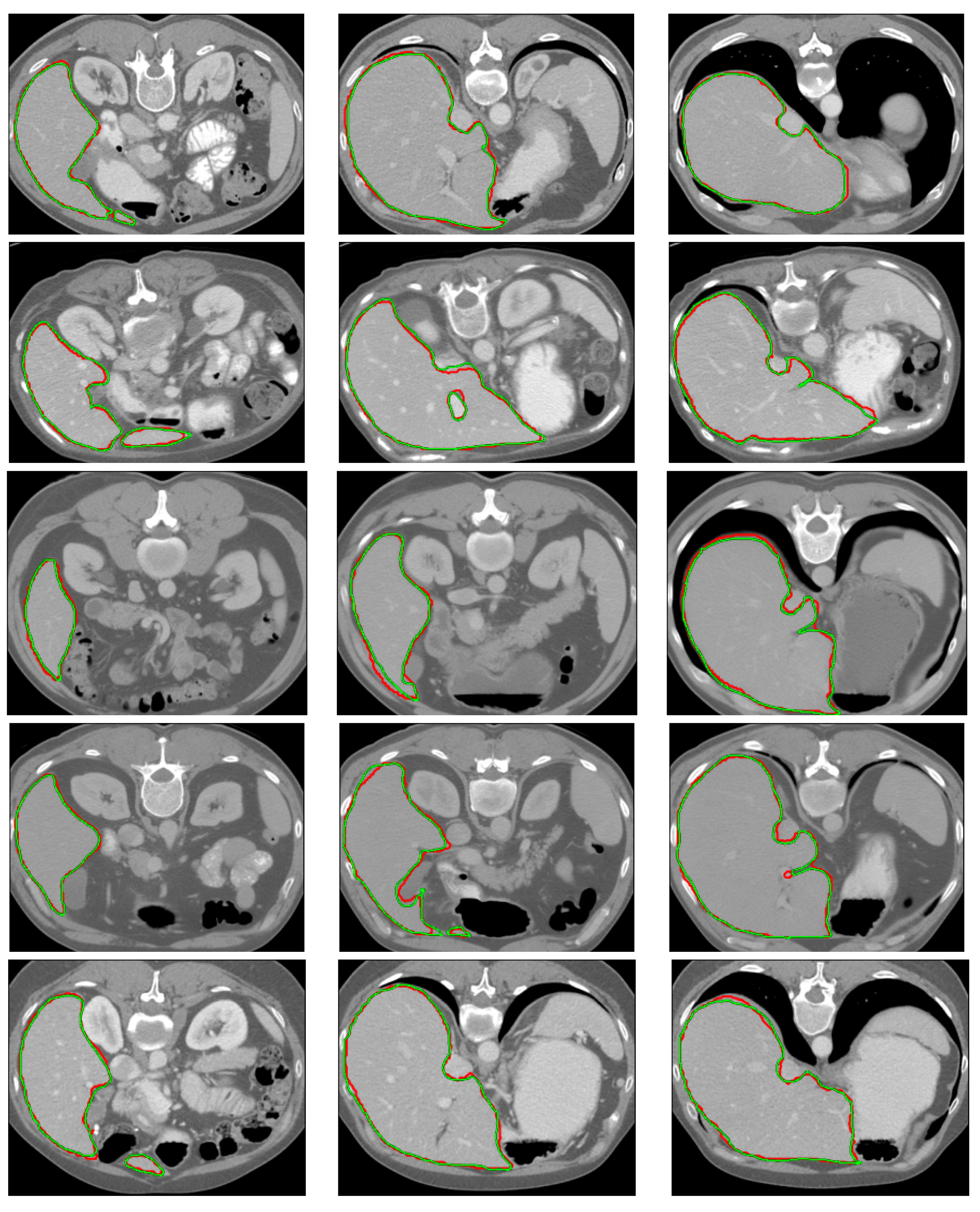
3.3. Results

Examples of segmentation results and the corresponding ground truth annotations are shown in Figure 8. Recall that the dataset that we are using, with the reference segmentations, are provided by [36]. They have set up their experiments with 9-fold cross-validation, and have manually cropped the images to their region of interest. We performed our experiments with 4-fold cross-validation and report results on two types of data: the cropped data, using coordinates provided by [36], and the whole slice subvolume containing all annotations. Like [36], our results are upsampled and the metrics are computed at the original CT resolution unless otherwise specified. Also similar to [36], we did not include this upsampling time in the segmentation time.

Table 1. 3D CVNN-UNet and Deep Chan-Vese 3D evaluation. Deep Chan-Vese 3D is estimated both at the inference resolution and full resolution. Metrics are calculated in two regions; “whole”: on all the slices that are annotated and with the whole axial plane, “ROI”: based on the cropping regions used by DEEDS [42] + JLF [43] and DenseVNet [36]. The 3D CVNN-UNet was fed in ${\phi }^0$ with an average Dice score of 87.58.

Architecture	Inference	Upsampled	Metric	Dice	Boundary	95% Hausdorff	Segment.
	Size	to	Region		Err (mm)	Distance (mm)	Time (s)
3D CVNN-UNet	$128\times 128$	-	whole	95.58	1.77	4.45	1.25
	$128\times 128$	-	ROI	95.56	1.67	4.42	0.53
Deep Chan-Vese 3D	$256\times 256$	-	whole	95.59	1.71	4.45	0.26
	$256\times 256$	$512\times 512$	whole	95.07	1.59	4.53	0.26
	$256\times 256$	-	ROI	95.39	1.58	4.42	0.11
	$256\times 256$	$512\times 512$	ROI	95.24	1.49	4.40	0.11

shows the evaluation of the low resolution 3D CVNN U-Net and the medium resolution Deep Chan-Vese 3D on the cropped data (ROI) and the whole slice subvolumes. With only 353k parameters, the 3D CVNN-UNet achieved a median Dice coefficient of $95.58$ at $128\times 128$, $95.56$ within the ROI of [36], and $95.10$ when upsampled to $256\times 256$ without any other processing. Furthermore, the proposed Deep Chan-Vese 3D method with the extra 3D CVNN medium resolution refinement module, with only 593 additional parameters obtains a median Dice score of $95.59$ at $256\times 256$ resolution. We see that the Dice coefficient and $95\%$ Haussdorf distance are about the same for the two methods, but the mean boundary error is slightly smaller for the Deep Chan-Vese 3D, especially after upsampling to the original resolution.

We compare our results with DEEDS [42]+JLF [43], a multi-atlas-based method, and nine Deep Learning-based methods: VoxResNet [44], VNet [45], DenseVNet [36], ObeliskNet [10], using the results reported in [36] and [10], SETR [15], CoTr [17], UNETR [16] as reported by UNETR, nnU-Net [11] and DISSM [28] as reported by DISSM. One must observe however that the ObeliskNet results [10] were reported only on the 43 (easier) TCIA volumes, not on all 90 volumes. The SETR, CoTr and UNETR results are evaluated on 30 BTCV volumes, while the nnU-Net and DISSM are tested on 13 volumes.

The comparison with the state of the art is shown in

Table 2. Comparison with the state of the art methods for liver segmentation on the 90-volume multi-organ dataset [36] and other datasets. The 9-fold cross-validation results are taken from [36], the 5-fold results are from [16] and the 1-fold from [28].

		x-val	Volumes		Boundary	95% Haussdorf	Segmentation
Arhitecture	res	Folds	Tested	Dice	Err (mm)	Distance (mm)	Time (s)
DEEDS [42]+JLF [43]	144	9	90	94	2.1	6.2	4740
VoxResNet [44]	144	9	90	95	2.0	5.2	$<1$
VNet [45]	144	9	90	94	2.2	6.4	$<1$
DenseVNet [36]	144	9	90	96	1.6	4.9	12
ObeliskNet [10]	144	4	43	95.4	-	-	$<1$
SETR [15]	96	5	30	95.4	-	-	25
CoTr [17]	96	5	30	96.3	-	-	19
UNETR [16]	96	5	30	97.1	-	-	12
nnU-Net [11]	128	1	13	96.4	1.7	-	10
DISSM [28]	-	1	13	96.5	1.1	-	12
3D CVNN-UNet (ours)	128	4	90	95.6	1.67	4.42	0.53
Deep Chan-Vese 3D (ours)	256	4	90	95.2	1.49	4.40	0.64

. Our results are evaluated on the same cropped data from [36]. Besides the Dice coefficients, symmetric boundary error and 95% Haussdorf distance, Table 2 also shows the number of cross-validation folds and the number of volumes each method was evaluated on, as well as the computation time.

In terms of Dice coefficients, our method is better than DEEDS+JLF and VNet, and comparable to VoxResNet, ObeliskNet [10] (Evaluated only on the 43 TCIA volumes), SETR [15], and DenseVNet [36] (since they only reported 2 decimals, their results could be anywhere in the interval $[95.5,96.49]$). It is outperformed by nnU-Net (Evaluated on 13 MSD [46] volumes, as reported by [28].The nnU-Net authors did not report metrics on Liver), DISSM (Used 118 volumes from the MSD [46] liver dataset to train and validate their method, and the remaining 13 MSD volumes for testing their method as well as nnU-Net [11]) and the transformer-based methods CoTr and UNETR. However, the nnU-Net and DISSM results are tested on only 13 volumes of a larger dataset, and should be taken with a grain of salt. Also, the SETR, CoTr and UNETR results are evaluated on only 30 volumes as opposed to our method, which is evaluated on 90 volumes. Moreover, half of the volumes that we have evaluated our method on come from pathological cases with cancerous lesions, which makes the segmentation task more challenging.

However, in terms of boundary error and $95\%$ Hausdorf distance our Deep Chan-Vese 3D outperforms all the competing methods that have the respective measure evaluated, except DISSM for the boundary error.

In terms of computing time, our method is on par with the deep learning methods VoxResNet and VNet, is faster than the transformer-based methods SETR, CoTr and UNETR as well as DenseVNet and DISSM, and is much faster than the atlas-based DEEDS+JLF.

3.4. Ablation Study

In this ablation study, we investigate the contribution of the 3D approach vs. an equivalent 2D approach and also of the 3D CVNN-UNet vs. a simple 3D CVNN. The data used in this study are same as in the rest of the paper. For 2D inputs we used medium resolution input, i.e., $256\times 256$, same as in Section 2.2, and for the 3D experiments the small resolution data are used, i.e., $128\times 128\times k$, same as in Section 2.3.1. The results are shown in

Table 3. Ablation results comparing 2D vs. 3D approaches and CNN vs UNet. The results are shown as average Dice scores obtained with 4-fold cross-validation.

	3D	U-Net	${\mathit{\phi }}^0$	1-it	2-it	3-it	4-it
2D CVNN	-	-	87.58	92.75	93.66	93.63	93.68
2D CVNN-UNet	-	+	87.58	92.61	93.72	93.63	93.75
3D CVNN	+	-	87.58	88.29	90.23	91.43	91.74
3D CVNN-UNet	+	+	87.58	92.83	94.41	95.09	95.52

.

The results from Table 3 show that the contributions of this paper (using a U-Net architecture instead of a CNN and working on 3D volumes instead of 2D slices) are essential for improving the quality of the results and bringing the Deep Chan-Vese formulation to state of the art performance. More 2D experiments are available in [47].

4. Conclusions

This paper presented a method for 3D liver segmentation that uses a Chan-Vese Neural Network combined with a 3D U-Net to achieve state of the art liver segmentation results. We showed how to provide a more appropriate input for the 3D CVNN-UNet in the form of a probability map and how to use a pixelwise detection map for initialization. We also showed multiple types of data augmentation as initialization when training the 3D CVNN-UNet to avoid overfitting.

In contrast to standard neural networks and recurrent neural networks, the Chan-Vese NN uses the U-Net as a shape model and has intensity models with latent parameters for the foreground and background regions, which are updated at each iteration of the segmentation procedure. This allows the whole U-Net to have fewer parameters than the standard models used for organ segmentation. In the future we plan to extend our method to multi-organ segmentation with separate shape models for each organ.

References

- Chan, T.F.; Vese, L.A. Active Contours without Edges. IEEE Trans. Image Process. 2001, 10, 266–277. [Google Scholar] [CrossRef] [PubMed]
- Akal, O.; Barbu, A. Learning Chan-Vese. In Proceedings of the ICIP, Taipei, Taiwan, 22–25 September 2019; IEEE: Piscataway, NJ, USA, 2019; pp. 1590–1594. [Google Scholar]
- Ronneberger, O.; Fischer, P.; Brox, T. U-net: Convolutional networks for biomedical image segmentation. In Proceedings of the MICCAI, Munich, Germany, 5–9 October 2015; Springer: Berlin/Heidelberg, Germany, 2015; pp. 234–241. [Google Scholar]
- Çiçek, Ö.; Abdulkadir, A.; Lienkamp, S.S.; Brox, T.; Ronneberger, O. 3D U-Net: Learning dense volumetric segmentation from sparse annotation. In Proceedings of the MICCAI, Athens, Greece, 17–21 October 2016; Springer: Berlin/Heidelberg, Germany, 2016; pp. 424–432. [Google Scholar]
- Oktay, O.; Schlemper, J.; Folgoc, L.L.; Lee, M.; Heinrich, M.; Misawa, K.; Mori, K.; McDonagh, S.; Hammerla, N.Y.; Kainz, B.; et al. Attention u-net: Learning where to look for the pancreas. arXiv 2018, arXiv:1804.03999. [Google Scholar]
- Zhou, Z.; Siddiquee, M.M.R.; Tajbakhsh, N.; Liang, J. Unet++: A nested u-net architecture for medical image segmentation. In Deep Learning in Medical Image Analysis and Multimodal Learning for Clinical Decision Support; Springer: Berlin/Heidelberg, Germany, 2018; pp. 3–11. [Google Scholar]
- Akal, O.; Peng, Z.; Hermosillo Valadez, G. ComboNet: Combined 2D and 3D architecture for aorta segmentation. arXiv 2020, arXiv:2006.05325. [Google Scholar]
- Guerrero, R.; Qin, C.; Oktay, O.; Bowles, C.; Chen, L.; Joules, R.; Wolz, R.; Valdés-Hernández, M.d.C.; Dickie, D.; Wardlaw, J.; et al. White matter hyperintensity and stroke lesion segmentation and differentiation using convolutional neural networks. Neuroimage Clin. 2018, 17, 918–934. [Google Scholar] [CrossRef]
- He, K.; Zhang, X.; Ren, S.; Sun, J. Deep residual learning for image recognition. In Proceedings of the CVPR, Las Vegas, NV, USA, 27–30 June 2016; pp. 770–778. [Google Scholar]
- Heinrich, M.P.; Oktay, O.; Bouteldja, N. OBELISK-Net: Fewer layers to solve 3D multi-organ segmentation with sparse deformable convolutions. Med. Image Anal. 2019, 54, 1–9. [Google Scholar] [CrossRef]
- Isensee, F.; Jäger, P.F.; Full, P.M.; Vollmuth, P.; Maier-Hein, K.H. nnU-Net for brain tumor segmentation. In Proceedings of the International MICCAI Brainlesion Workshop, Lima, Peru, 4 October 2020; Springer: Berlin/Heidelberg, Germany, 2020; pp. 118–132. [Google Scholar]
- Kenton, J.D.M.W.C.; Toutanova, L.K. BERT: Pre-training of Deep Bidirectional Transformers for Language Understanding. In Proceedings of the NAACL-HLT, Minneapolis, Minnesota, 2–7 June 2019; pp. 4171–4186. [Google Scholar]
- Carion, N.; Massa, F.; Synnaeve, G.; Usunier, N.; Kirillov, A.; Zagoruyko, S. End-to-end object detection with transformers. In Proceedings of the European Conference on Computer Vision, Glasgow, UK, 23–28 August 2020; Springer: Berlin/Heidelberg, Germany, 2020; pp. 213–229. [Google Scholar]
- Dosovitskiy, A.; Beyer, L.; Kolesnikov, A.; Weissenborn, D.; Zhai, X.; Unterthiner, T.; Dehghani, M.; Minderer, M.; Heigold, G.; Gelly, S.; et al. An image is worth 16x16 words: Transformers for image recognition at scale. arXiv 2020, arXiv:2010.11929. [Google Scholar]
- Zheng, S.; Lu, J.; Zhao, H.; Zhu, X.; Luo, Z.; Wang, Y.; Fu, Y.; Feng, J.; Xiang, T.; Torr, P.H.; et al. Rethinking semantic segmentation from a sequence-to-sequence perspective with transformers. In Proceedings of the IEEE/CVF Conference on Computer Vision and Pattern Recognition, Nashville, TN, USA, 20–25 June 2021; pp. 6881–6890. [Google Scholar]
- Hatamizadeh, A.; Tang, Y.; Nath, V.; Yang, D.; Myronenko, A.; Landman, B.; Roth, H.R.; Xu, D. Unetr: Transformers for 3d medical image segmentation. In Proceedings of the IEEE/CVF Winter Conference on Applications of Computer Vision, Waikoloa, HI, USA, 3–8 January 2022; pp. 574–584. [Google Scholar]
- Xie, Y.; Zhang, J.; Shen, C.; Xia, Y. Cotr: Efficiently bridging cnn and transformer for 3d medical image segmentation. In Proceedings of the MICCAI, Strasbourg, France, 27 September–1 October 2021; Springer: Berlin/Heidelberg, Germany, 2021; pp. 171–180. [Google Scholar]
- Ngo, T.A.; Lu, Z.; Carneiro, G. Combining deep learning and level set for the automated segmentation of the left ventricle of the heart from cardiac cine magnetic resonance. Med. Image Anal. 2017, 35, 159–171. [Google Scholar] [CrossRef]
- Mohamed, A.r.; Dahl, G.E.; Hinton, G. Acoustic modeling using deep belief networks. IEEE Trans. Audio Speech Lang. Process. 2011, 20, 14–22. [Google Scholar] [CrossRef]
- Otsu, N. A threshold selection method from gray-level histograms. IEEE Trans. Syst. Man Cybern. 1979, 9, 62–66. [Google Scholar] [CrossRef]
- Li, C.; Xu, C.; Gui, C.; Fox, M.D. Distance regularized level set evolution and its application to image segmentation. IEEE Trans. Image Process. 2010, 19, 3243–3254. [Google Scholar] [CrossRef]
- Hu, P.; Shuai, B.; Liu, J.; Wang, G. Deep level sets for salient object detection. In Proceedings of the CVPR, Honolulu, HI, USA, 21–26 July 2017; pp. 2300–2309. [Google Scholar]
- Hu, P.; Wang, G.; Kong, X.; Kuen, J.; Tan, Y.P. Motion-guided cascaded refinement network for video object segmentation. In Proceedings of the CVPR, Salt Lake City, UT, USA, 18–23 June 2018; pp. 1400–1409. [Google Scholar]
- Simonyan, K.; Zisserman, A. Very deep convolutional networks for large-scale image recognition. arXiv 2014, arXiv:1409.1556. [Google Scholar]
- Hancock, M.C.; Magnan, J.F. Lung nodule segmentation via level set machine learning. arXiv 2019, arXiv:1910.03191. [Google Scholar]
- He, K.; Gkioxari, G.; Dollár, P.; Girshick, R. Mask r-cnn. In Proceedings of the IEEE International Conference on Computer Vision, Venice, Italy, 22–29 October 2017; pp. 2961–2969. [Google Scholar]
- Homayounfar, N.; Xiong, Y.; Liang, J.; Ma, W.C.; Urtasun, R. Levelset r-cnn: A deep variational method for instance segmentation. In Proceedings of the European Conference on Computer Vision, Glasgow, UK, 23–28 August 2020; Springer: Berlin/Heidelberg, Germany, 2020; pp. 555–571. [Google Scholar]
- Raju, A.; Miao, S.; Jin, D.; Lu, L.; Huang, J.; Harrison, A.P. Deep implicit statistical shape models for 3d medical image delineation. In Proceedings of the AAAI Conference on Artificial Intelligence, Virtual, 22 February–1 March 2022; Volume 36, pp. 2135–2143. [Google Scholar]
- Tripathi, S.; Singh, S.K. An Object Aware Hybrid U-Net for Breast Tumour Annotation. arXiv 2022, arXiv:2202.10691. [Google Scholar]
- Mumford, D.; Shah, J. Optimal approximations by piecewise smooth functions and associated variational problems. Commun. Pure Appl. Math. 1989, 42, 577–685. [Google Scholar] [CrossRef]
- Paszke, A.; Gross, S.; Chintala, S.; Chanan, G.; Yang, E.; DeVito, Z.; Lin, Z.; Desmaison, A.; Antiga, L.; Lerer, A. Automatic differentiation in PyTorch. In NeurIPS Autodiff Workshop; 2017; Available online: https://openreview.net/pdf?id=BJJsrmfCZ (accessed on 13 September 2022).
- Taghanaki, S.A.; Zheng, Y.; Zhou, S.K.; Georgescu, B.; Sharma, P.; Xu, D.; Comaniciu, D.; Hamarneh, G. Combo loss: Handling input and output imbalance in multi-organ segmentation. Comput. Med. Imaging Graph. 2019, 75, 24–33. [Google Scholar] [CrossRef]
- Sudre, C.H.; Li, W.; Vercauteren, T.; Ourselin, S.; Cardoso, M.J. Generalised dice overlap as a deep learning loss function for highly unbalanced segmentations. In Deep Learning in Medical Image Analysis and Multimodal Learning for Clinical Decision Support; Springer: Berlin/Heidelberg, Germany, 2017; pp. 240–248. [Google Scholar]
- Barbu, A. Training an active random field for real-time image denoising. IEEE Trans. Image Process. 2009, 18, 2451–2462. [Google Scholar] [CrossRef]
- Huang, G.; Li, Y.; Pleiss, G.; Liu, Z.; Hopcroft, J.E.; Weinberger, K.Q. Snapshot ensembles: Train 1, get M for free. arXiv 2017, arXiv:1704.00109. [Google Scholar]
- Gibson, E.; Giganti, F.; Hu, Y.; Bonmati, E.; Bandula, S.; Gurusamy, K.; Davidson, B.; Pereira, S.P.; Clarkson, M.J.; Barratt, D.C. Automatic multi-organ segmentation on abdominal CT with dense v-networks. IEEE Trans. Med. Imaging 2018, 37, 1822–1834. [Google Scholar] [CrossRef]
- Clark, K.; Vendt, B.; Smith, K.; Freymann, J.; Kirby, J.; Koppel, P.; Moore, S.; Phillips, S.; Maffitt, D.; Pringle, M.; et al. The Cancer Imaging Archive (TCIA): Maintaining and operating a public information repository. J. Digit. Imaging 2013, 26, 1045–1057. [Google Scholar] [CrossRef]
- Roth, H.R.; Farag, A.; Turkbey, E.B.; Lu, L.; Liu, J.; Summers, R.M. Data from pancreas-CT. Cancer Imaing Arch. 2016. [Google Scholar] [CrossRef]
- Roth, H.R.; Lu, L.; Farag, A.; Shin, H.C.; Liu, J.; Turkbey, E.B.; Summers, R.M. Deeporgan: Multi-level deep convolutional networks for automated pancreas segmentation. In Proceedings of the MICCAI, Munich, Germany, 5–9 October 2015; Springer: Berlin/Heidelberg, Germany, 2015; pp. 556–564. [Google Scholar]
- Landman, B.; Xu, Z.; Igelsias, J.; Styner, M.; Langerak, T.; Klein, A. MICCAI Multi-Atlas Labeling Beyond the Cranial Vault–Workshop and Challenge. 2015. Available online: https://www.synapse.org/#!Synapse:syn3193805/files/ (accessed on 13 September 2022).
- Xu, Z.; Lee, C.P.; Heinrich, M.P.; Modat, M.; Rueckert, D.; Ourselin, S.; Abramson, R.G.; Landman, B.A. Evaluation of six registration methods for the human abdomen on clinically acquired CT. IEEE Trans. Biomed. Eng. 2016, 63, 1563–1572. [Google Scholar] [CrossRef] [PubMed]
- Heinrich, M.P.; Jenkinson, M.; Brady, M.; Schnabel, J.A. MRF-based deformable registration and ventilation estimation of lung CT. IEEE Trans. Med. Imaging 2013, 32, 1239–1248. [Google Scholar] [CrossRef] [PubMed]
- Wang, H.; Suh, J.W.; Das, S.R.; Pluta, J.B.; Craige, C.; Yushkevich, P.A. Multi-atlas segmentation with joint label fusion. IEEE Trans. PAMI 2012, 35, 611–623. [Google Scholar] [CrossRef] [PubMed]
- Chen, H.; Dou, Q.; Yu, L.; Heng, P.A. Voxresnet: Deep voxelwise residual networks for volumetric brain segmentation. arXiv 2016, arXiv:1608.05895. [Google Scholar]
- Milletari, F.; Navab, N.; Ahmadi, S.A. V-net: Fully convolutional neural networks for volumetric medical image segmentation. In Proceedings of the International Conference on 3D Vision (3DV), Stanford, CA, USA, 25–28 October 2016; IEEE: Piscataway, NJ, USA, 2016; pp. 565–571. [Google Scholar]
- Simpson, A.L.; Antonelli, M.; Bakas, S.; Bilello, M.; Farahani, K.; Van Ginneken, B.; Kopp-Schneider, A.; Landman, B.A.; Litjens, G.; Menze, B.; et al. A large annotated medical image dataset for the development and evaluation of segmentation algorithms. arXiv 2019, arXiv:1902.09063. [Google Scholar]
- Akal, O. Deep Learning Based Generalization of Chan-Vese Level Sets Segmentation. Ph.D. Thesis, Florida State University, Tallahassee, FL, USA, 2020. Order No. 28022313. [Google Scholar]