Article

Techno-Economic Evaluation of Hybrid Energy Systems Using Artificial Ecosystem-Based Optimization with Demand Side Management

by
Hammed Olabisi Omotoso
*,
Abdullah M. Al-Shaalan
,
Hassan M. H. Farh
and
Abdullrahman A. Al-Shamma’a
*
Electrical Engineering Department, College of Engineering, King Saud University, Riyadh 11421, Saudi Arabia
*
Authors to whom correspondence should be addressed.
Electronics 2022, 11(2), 204; https://doi.org/10.3390/electronics11020204
Submission received: 9 November 2021 / Revised: 29 December 2021 / Accepted: 4 January 2022 / Published: 10 January 2022

Abstract

:
Electrification of remote rural areas by adopting renewable energy technologies through the advancement of smart micro-grids is indispensable for the achievement of continuous development goals. Satisfying the electricity demand of consumers while adhering to reliability constraints with docile computation analysis is challenging for the optimal sizing of a Hybrid Energy System (HES). This study proposes the new application of an Artificial Ecosystem-based Optimization (AEO) algorithm for the optimal sizing of a HES while satisfying Loss of Power Supply Probability (LPSP) and Renewable Energy Fraction (REF) reliability indices. Furthermore, reduction of surplus energy is achieved by adopting Demand Side Management (DSM), which increases the utilization of renewable energy. By adopting DSM, 28.38%, 43.05%, and 65.37% were achieved for the Cost of Energy (COE) saving at 40%, 60%, and 80% REF, respectively. The simulation and optimization results demonstrate the most cost-competitive system configuration that is viable for remote-area utilization. The proposed AEO algorithm is further compared to Harris Hawk Optimization (HHO) and the Future Search Algorithm (FSA) for validation purpose. The obtained results demonstrate the efficacy of AEO to achieve the optimal sizing of HES with the lowest COE, the highest consistent level, and minimal standard deviation compared with HHO and FSA. The proposed model was developed and simulated using the MATLAB/code environment.

Graphical Abstract

1. Introduction

The reduction of conventional energy sources coupled with increasing global warming have accelerated the growth of renewable energy sources (RES) such as solar and wind [1]. RES can be exploited for both grid connection and for off-grid, especially in rural areas with restricted grid connection [2,3,4]. This will reduce fossil fuel dependency, harmful emissions, and consumption costs. In spite of their benefits, RES performance is often limited due to the intermittent and unpredictable nature of their output power [5]. These factors affects both energy production and the operational costs of the system. Connecting two or more RES is essential to sustain energy for remote areas by preserving the quality and reliability of power [6]. Likewise, incorporating diesel generators with RES can ensure service quality and reliability and results in less battery maintenance [7,8]. Therefore, it is essential to optimize Hybrid Energy System (HES) size to minimize installation and maintenance cost.
Several studies have adopted analytical, probabilistic, and heuristic techniques in achieving HES optimization. The probabilistic technique is modelled on the random prospect of a particular system [9,10]. However, this method is not robust for obtaining optimal result with dynamic change in RES. The analytical technique is only capable of handling simple and precise methods [11,12]. The potent results of the heuristic methods [13,14,15,16,17,18,19,20] make them dependable for complex optimal sizing of HES with sufficient computational time. In [13], the Harmony Search (HS) algorithm was utilized for sizing PV/diesel energy sources. The obtained result in [13] demonstrated the robustness of HS in reducing pollution and system cost. Masoud et al. [14] demonstrated the effectiveness of Dynamic Multi-Objectives Particle Swarm Optimization (DMOPSO) for sizing the HES. By utilizing the DMOPSO algorithm, the results revealed a decrease in PV panel cost and NPC. In [15], a genetic algorithm combined with particle swarm optimization was used for the optimal design of a hybrid wind–PV–battery system. Loss of Load Expected (LOLE) and Loss of Energy Expected (LOEE) were subjected to constraints to minimize operation cost using multi-objective particle swarm optimization [16]. Eftichios et al. [17] presented a genetic algorithm using the system cost function subject to Loss of Load Hours (LOLH) constraints for HES optimization. Minimization of COE is presented in [18] to optimize the size of the HES subject to Renewable Energy Fraction (REF) and LPSP constraints. In [17], the levelized cost of energy was obtained through optimal sizing of PV, wind, battery, and diesel generator. Wang et al. [20] proposed a non-dominated sorting algorithm II, incorporated with re-ranking based genetic operators to determine system reliability, greenhouse gas emission, and lifetime cost for optimal sizing of the HES. Crow Search (CS) and Particle Swarm Optimization (PSO) were introduced in [21,22] for optimal sizing and allocation of renewable distributed generations. Morteza et al. presented a solar-hydrogen model for hybrid energy sizing using Demand Side Management (DSM) [23]. The results revealed the decrease in electricity cost; however, the model did not utilize system constraints. Hassan et al. [24] presented a strategy to allocate renewable distributed generations using CS with PSO.
The majority of the optimal sizing of HES in the literature did not apply DSM concepts. DSM is the future of power systems, incorporating cutting-edge technologies and distributions system for supplying electricity in efficient and smart ways [25]. DSM buttresses smart grid in several ways, such as control, electricity cost reduction, monitoring, and management of energy resources [26]. DSM can help to reduce load peak, which increases the efficiency of grid operation, promotes a decrease in the greenhouse gas effect, and leads to electricity bill reduction. Effective DSM can avoid the upgrading of electrical infrastructures such as transmission lines and distribution networks. Some of the generic method of DSM [27] are valley filling, load conservation, peak clipping, load growth or load establishment, and load shifting. Peak clipping is the reduction of peak loads without shifting it to off-peak hours. Valley filling involves encouraging consumption during the off-peak period. Load conservation involves encouraging consumers to make use of efficient appliances to reduce energy wastage. Load growth is adopted in a situation of surplus energy that might be the result of the integration of renewable energy. Load shifting is most commonly utilized and involves the shifting of load from peak periods to off-peak periods or periods where the energy cost is cheap [27]. Cost saving is the major purpose of the load-shifting process [28]. This method will be utilized in this study for the optimal sizing of the HES. Figure 1a–d shows a pictorial representation of various DSM strategies.
Thus, the foremost objective of this study is to extend the work presented in [29] by incorporating DSM for the optimal sizing of HES for remote communities of Al Sulaymaniyah village, Saudi Arabia, using a new optimization algorithm. The evaluation of three algorithms: Artificial Ecosystem-based Optimization (AEO) [30], Future Search Algorithm (FSA) [31], Harris Hawk Optimization (HHO) [32], were evaluated for optimal sizing. These algorithms were analyzed for optimizing Cost of Energy (COE) at zero Loss of Power Supply Probability (LPSP). Additionally, the Renewable Energy factor is proposed to ensure a hybrid energy utilization among the energy sources: diesel, battery storage, PV, and wind. The results demonstrated the efficacy of AEO in obtaining the lowest COE with and without DSM.
The novelty and contribution of this paper can be summarized as follows:
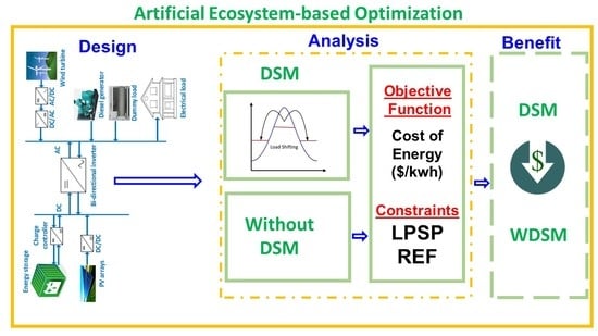
  • A new application of Artificial Ecosystem-based Optimization is utilized for the first time to achieve optimal sizing of HES by minimizing the Cost of Energy (COE);
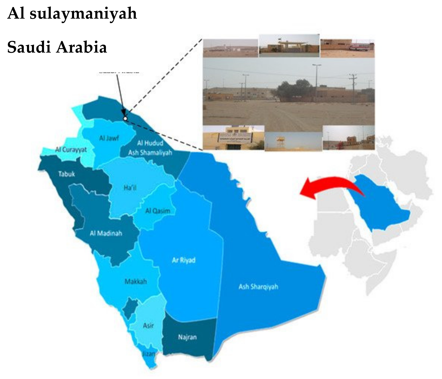
  • Renewable Energy Fraction (REF) and Loss of Power Supply Probability (LPSP) are utilized to achieve stand-alone HES consisting of PV/WTGs/battery/diesel for Al Sulaymaniyah village, Saudi Arabia;
  • A load-shifting strategy based on the available renewable is employed for the DSM to achieve a minimal cost of energy;
  • AEO is compared to FSA and HHO with DSM and without DSM in achieving the COE and to verify its efficacy;
  • Different values of REF at 40%, 60%, and 80% are utilized as constraints to determine the COE with DSM and without DSM;
  • The results demonstrated the effectiveness of AEO to achieve the lowest COE, both with DSM and without DSM.
The rest of the paper is arranged as follows: Section 2 describes the Al Sulaymaniyah site and load; Section 3 proposes the HES configuration; Section 4 discusses the AEO algorithm; Section 5 describes the power management approach; Section 6 introduces the developed DSM; Section 7 describes the reliability indices; Section 8 illustrates the objective function; Section 9 discusses the results; and Section 10 presents the conclusion.

2. Al Sulaymaniyah Site Description and Meteorological Data

The geographical location of Al Sulaymaniyah is shown in Figure 2 [29]. The village is located in the northern part of Saudi Arabia at an elevation of 1820 ft above sea level. The location has enormous availability of wind and solar energy. Al Sulaymaniyah village comprises mosques, a water pump, a small hospital, and recreation facilities. The village is supplied through diesel generators by the Saudi Electricity Company (SEC). The climatic conditions at the village are continental. The village’s temperature ranges between 0 °C and 45 °C throughout the year. The summer period is usually from May to September, while the winter season is from November to February. The day period varies throughout the year. The lengthiest day occurs in June, with 14 h of sunlight, and the shortest day occurs in December, with 10 h of sunlight.
The measured average hourly energy consumption at Al Sulaymaniyah village comprises 8760 data points. Currently, the village is powered by three 456 kW diesel generators connected in parallel to a common bus. The generated power is connected to a 1250 kVA step-up transformer. The full description of Al Sulaymaniyah meteorological data and load pattern are described in [29].

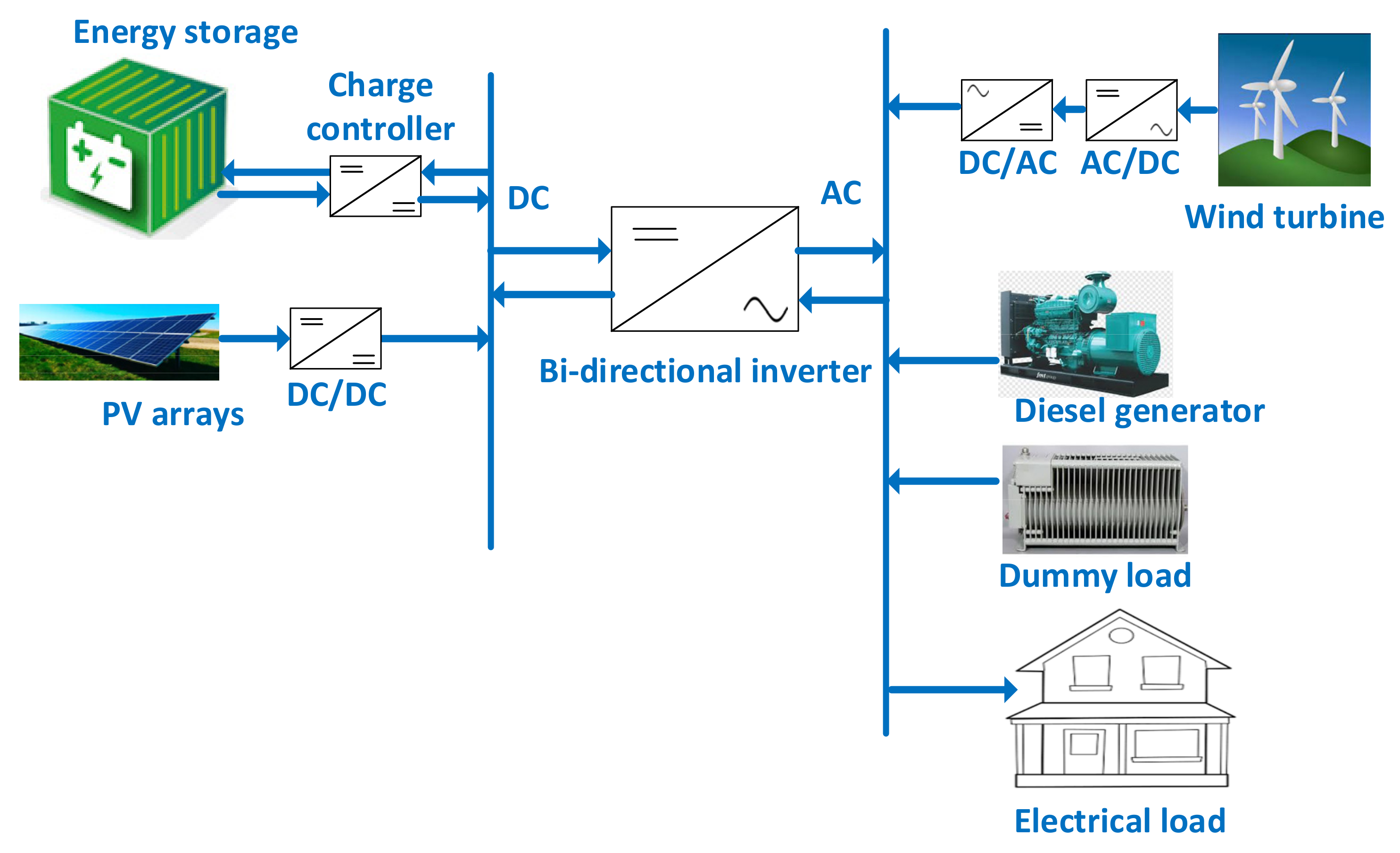
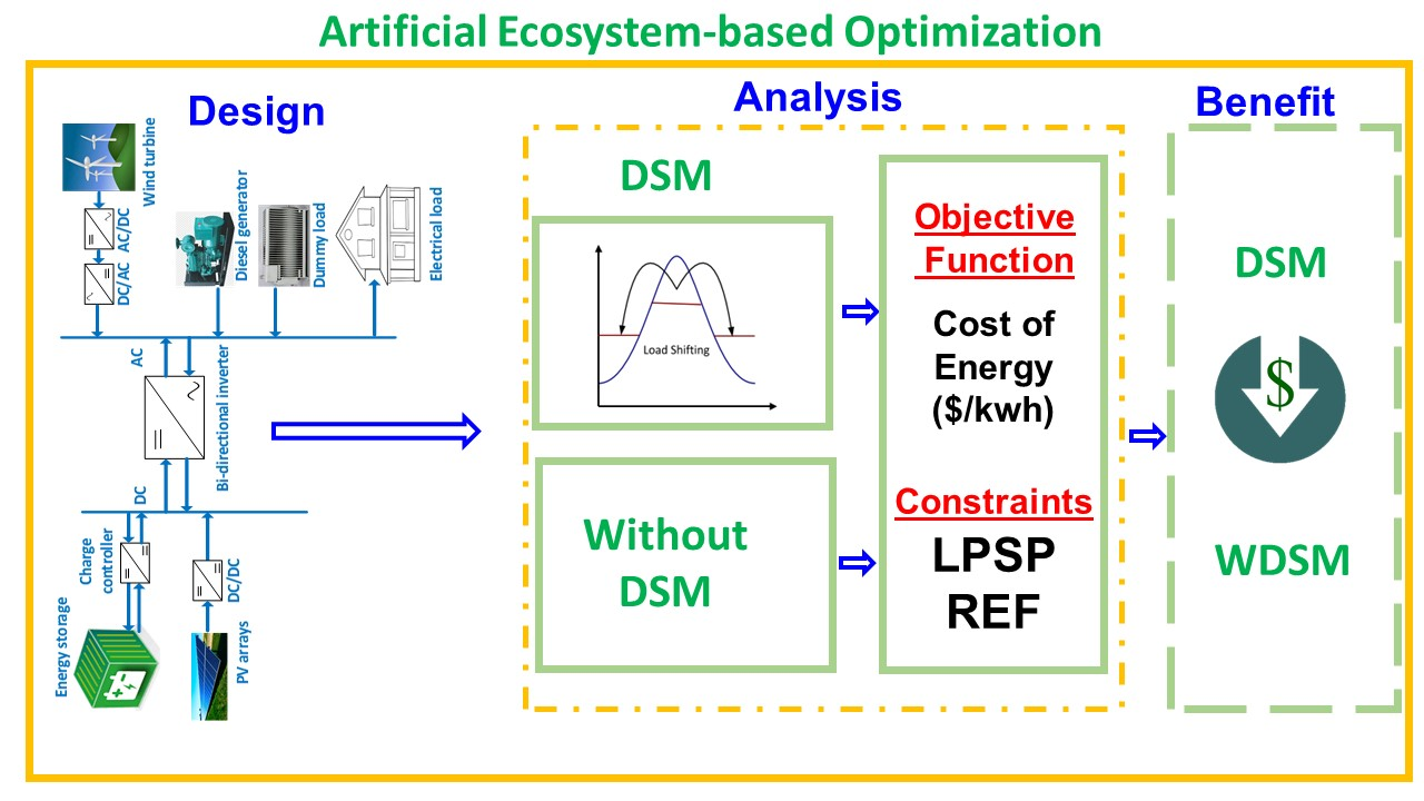
3. Configuration of the HES

The proposed structure for the Hybrid Energy System is presented in Figure 3 [33]. This comprises battery storage, the inverter for converting DC energy sources to AC, diesel generators, load, PV, and wind energy sources. In this study, PV and wind are considered as the two major sources of energy. Either the diesel generator or storage energy system compensates the disparity between PV and wind. Al Sulaymaniyah’s low PV and wind coefficient of correlation implies that PV and wind might not be able to adequately supply the energy required without the utilization of energy storage and diesel sources. PV and storage system are connected to the DC side of the bus bar, while the diesel generator and wind turbines are linked to the AC side of the bus bar. The diesel generator serves as an alternative source of energy whenever the PV, wind, and storage system are unable to meet the load demand.
The modelling of the PV, wind, storage system, and diesel generator is introduced as follows.

3.1. PV Modelling

Solar irradiance, PV array manufacturer’s data, and temperature are major factors that influence the output power generated from PV systems, as shown in (1) [34].
P P V =   P r f p v G T ¯ G T , S T C ¯ 1 + α p T c T c , S T C
where P r , T c , S T C , T c , G T ¯ , G T , S T C ¯ , α p , and f p v are the PV rated power, PV temperatures under STC and normal conditions, global irradiance under normal and Standard Test Conditions (STCs), power temperature coefficient, and de-rating factor, respectively. The temperature of the PV steady-state operation is described in (2).
T c = T a + N O C T T a ,   N O C T 1 1.11 η M P P ( 1 α p T c , S T C ) G T ¯ G T , N O C T 1 + 1.11 α ρ η M P P , S T C   N O C T T a , N O C T G T ¯ G T , N O C T
where N O C T and T a are operating cell nominal and ambient temperature, respectively. G T , N O C T and T a , N O C T are, respectively, the solar irradiance and ambient temperature with respect to NOCT; η M P P and η M P P , S T C are the Maximum Power Point (MPP) efficiency of the PV module and efficiency under STCs, respectively.

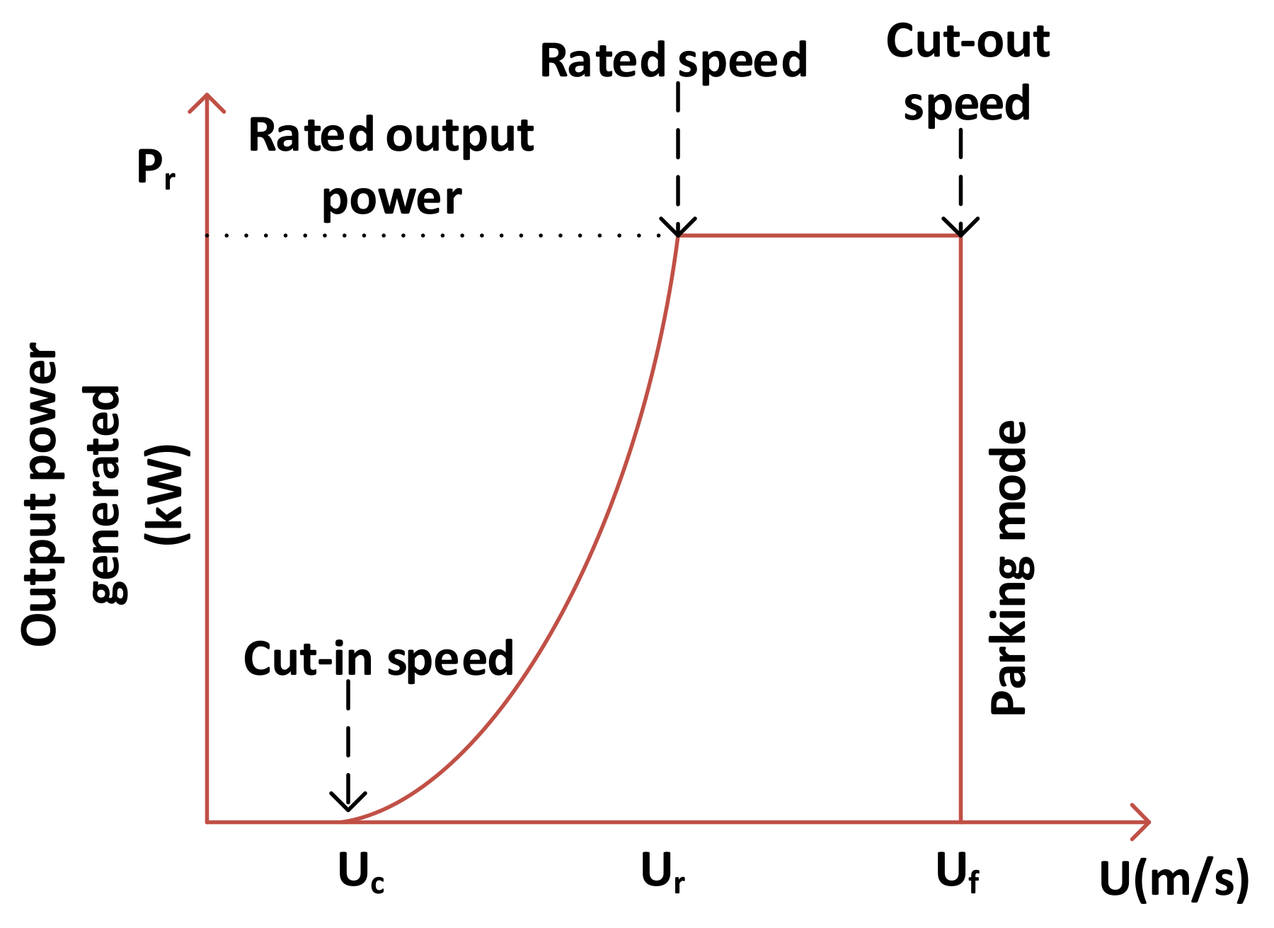
3.2. Wind Turbine Generator (WTG) Modelling

The approximated curve of power output of a wind turbine system can be expressed as follows [35]:
P W T u = P r × 0 u u c   o r   u > u f u 2 u c 2   u r   2 u c 2 u c < u u r 1 u r u u f
where u , u c , P r , u r , and u f are wind speed, cut-in/starting speed of wind turbine, rated power of wind turbine, rated speed, and cut-out/furling speed, respectively. It is evident from Equation (3) that wind turbine output power depends on five parameters, which are the four wind turbine parameters and the site wind speed ( u ). The four wind turbine parameters are u c , P r , u r , and u f . Based on a quadratic model, a typical wind turbine output power characteristic curve is shown in Figure 4 [29].

3.3. Storage System Modelling

One of the critical aspects of RES is the storage system because of the stochastic nature of RES output power. The depth of discharge and battery bank nominal capacity are important factors to be considered in storage system. The load demand determines the energy flow through the storage system. The State of Charge (SOC) of the battery bank is represented as (4) [29].
S O C t = S O C t 1 1 σ + P G A t P L   t η i n υ η b a t t e r y
where P L t , η i n υ , η b a t t e r y , P G A t , and σ are total load demand, net inverter efficiency, round trip efficiency of battery within [0.5, 0.95], total output power, and self-discharging rate, respectively. The charging and discharging operation of the storage system is described by the positive and negative second term of Equation (4). The constraints for the storage system State of Charge (SOC) are described in (5).
S O C t = S O C m i n S O C t < S O C m i n S O C t S O C min < S O C t < S O C m a x S O C m a x S O C t > S O C m a x
The SOC cannot exceed the maximum limit of S O C m a x , and likewise the minimum SOC must be equal to or exceed the minimum allowable limit, S O C m i n .

3.4. Diesel Generator

The diesel generator is utilized whenever the storage and RES is insufficient to sustain load demand. The annual fuel consumption and the cost is represented as (6) [35].
C D s l   = C F t = 1 8760 A × P D s l t + B   × P R
where C D s l , , P R , C F , and P D s l t are the annual fuel consumption (L/h), nominal power, cost of fuel per liter, and generated power (kW) of diesel, respectively. A , B are the fuel constants (L/kW). The two main import factor that influences the fuel consumption are both the output power and nominal power. The output power of the diesel generator is recommended by the manufacturers between a preset minimum level and nominal power.

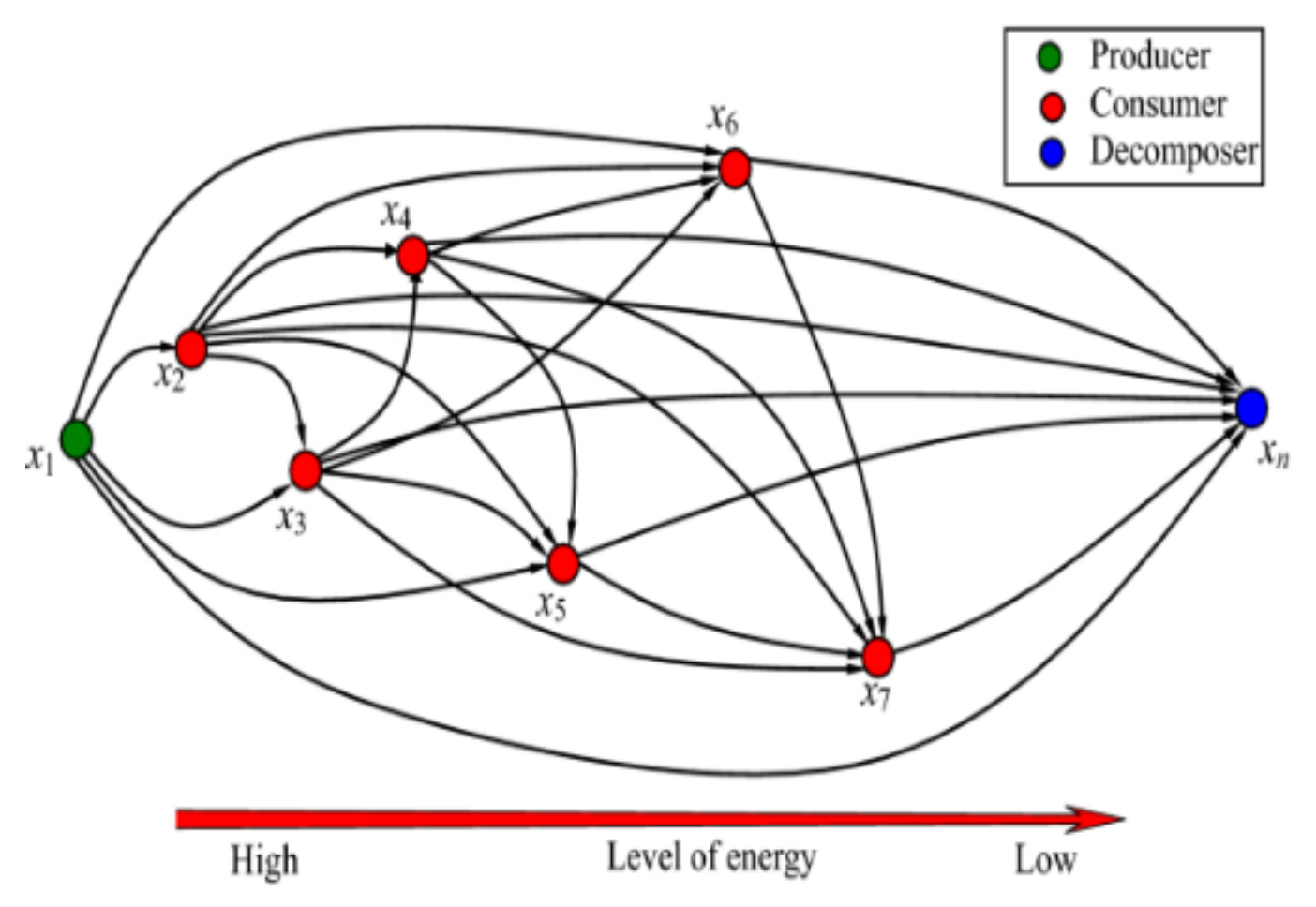
4. Artificial Ecosystem-Based Optimization (AEO)
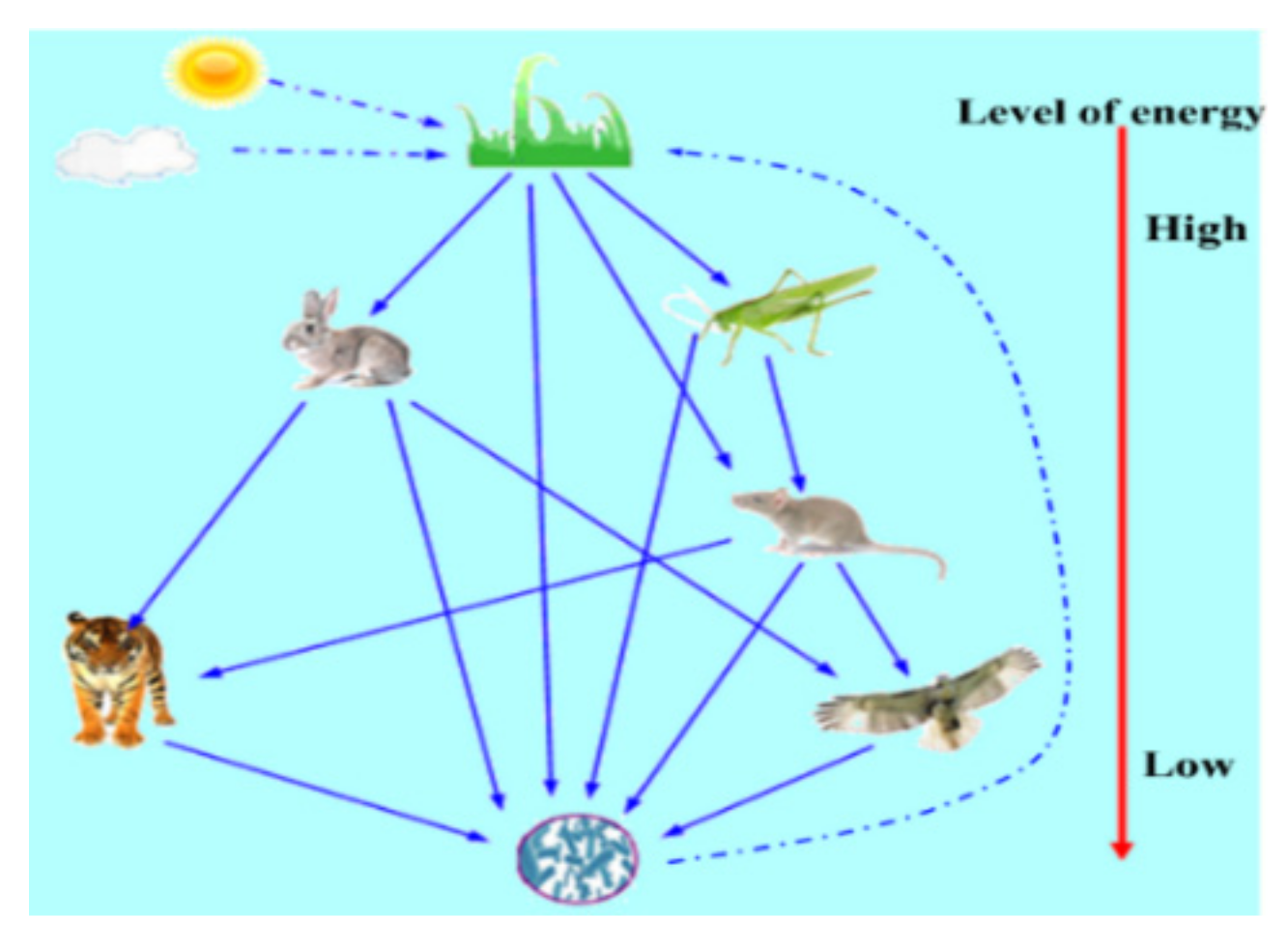
AEO is a type of population-based optimization algorithm. It imitates the production, decomposition, and consumption behavior of living organisms. This concept depicts energy flow in the ecosystem of the Earth. In the Earth’s ecosystem, producers use water, sunlight, and carbon dioxide to make food energy. Similarly, the AEO production stage is used to improve the balance between exploration and exploitation. The second stage, consumers, just like animals, cannot produce their own food. They acquire their energy and nutrients from fellow consumers or producers. This stage improves the exploration of the algorithm. Decomposition is the last stage. Decomposers feed on both consumers and producers. The exploitation of the algorithm is enriched at this stage [30].

4.1. Producer

In the search space at this stage, a random individual ( x r a n d i ) and a best individual ( x q ) are randomly produced. The decomposer (best individual) and the search space’s upper and lower boundaries update the producer (worst individual). This update will facilitate other individuals to hunt for separate regions. The mathematical representation for this is illustrated in (7) [30].
x 1 t i + 1 = 1 a x q t i + a x r a n d i t i
where
a = 1 t i I t r 1
x r a n d i = r U p L w + L w
x 2 t i + 1 = x 2 t i + K x 2 t i x 1 t i
where r 1 and r are random numbers within 0 and 1, I t is maximum iterations, a is linear weighting coefficient, q is the population number, and L w and U p are the lower and upper boundaries, respectively. The flight levy, K , is for enhancement of the exploration level. This is represented in (11) [36]:
K = 0.5 v 1 / v 2
where v 2 = N 0 , 1 and v 1 = N 0 , 1 . N 0 , 1 denotes normal distribution.

4.2. Consumption

This stage enhances the exploration by letting the algorithms upgrade the solution of individuals. The consumers can be classified as herbivore, carnivore, or omnivore. The herbivore feeds on both the consumers and the producers. The second feed on the consumers with an advanced energy level. The last feeds on the producers and/or consumers with an advanced energy level. The mathematical equation for herbivore as a consumer is represented as follows [36]:
x i t i + 1 = x i t i + K x i t i x i t i ,   i 3 , , n
The mathematical equation for consumer as a carnivore is represented as follows:
x i t i + 1 = x i t i + K x i t i x j t i , i 3 , , n ,   j = r a n d i 2   i 1
The mathematical equation for an omnivore consumer is denoted as:
x i t i + 1 = x i t i + K r 2 x i t i x 1 t i + 1 r 2 x i t i x j t i , i 3 , , n ,   j = r a n d i 2   i 1
where r 2 is within the range of 0 and 1.

4.3. Decomposers

The decomposition stage is very important because it feeds the producers and encompasses the food chain. In Earth’s ecosystem, when a consumer passes away, the decomposers feed on its leftovers. The mathematical Equation (15) for the decomposer model introduces new factors. The factors are weight coefficients ( w e   and   h e ) and decomposition factor ( D e ) . The decomposition supports the exploitation of the algorithm by updating individual locations based on the best solution, as described in (16) [30].
x i t i + 1 = x n t i + D e w e x n t i h e x i t t ,   i = 1 , , n
The newly introduced factors are defined by Equation (16), shown below.
D e = 3 u , u N 0 , 1 w e = r 3 r a n d i 1 , 2 1 h e = 2 r 3 1
where r 3 is within the range of 0 and 1.

4.4. Termination

During this stage, x q is updated after the fitness is obtained for each individual. Subsequently, the termination condition is evaluated; if it is met, the execution is terminated and x q is returned, or else the first stage is repeated. Figure 5 and Figure 6 show the typical flow of energy in Earth’s ecosystem and the AEO ecosystem [30], and Algorithm 1 summarized the pseudocode AEO algorithm.
Algorithm 1: Pseudocode of Artificial Ecosystem-based Optimization for optimal the sizing of HES
1. Initialization: Random initialization of AEO ecosystem, x1, and evaluation of fitness, ffi; xq = best solution established so far.
2. While the halt condition is not obtained, perform:
  First Stage: Production
   Individual x1, update its position with (7).
  Second Stage: Consumption
   Individual x1 (i = 2, …,n)
  Herbivorous act occurs
   If r a n d < 1 3 , the individual update is carried out using (12)
  Omnivorous act occurs
   Else if 1/3 and rand < 2/3 the update to individual is carried out using (14)
  Carnivorous act occurs
   Else the individual update is carried out with (13)
   End if
  End if
  Third stage: Decomposition
    Individual update is carried out with (15)
    Individual fitness is calculated
    Best position found so far is updated, xq
    End while
  Fourth Stage: Termination
    Return xq

5. Power Management Approach

The unstable nature of renewable resources creates a multifaceted power management scheme for HES. Due to the fact that the quantity of energy generated from resources is paltry, the capability of the generator cannot be instantaneously amplified to balance the increase in load. Moreover, occasionally, a dump load is required to dispel the surplus when the quantity of electricity generated is more than the demand. Moreover, this will avoid the overcharging of the batteries. To design an effective system, it is essential to adopt a power management methodology. Table 1 shows the parameters used for the simulation [35]. The following cases are considered for the power management methodology.
Case 1: The required energy is supplied by renewable generation and the surplus is utilized for charging the storage facility.
Case 2: As in Case 1, if the excess energy is greater than the storage capacity and load, the surplus is dissipated via a dump load.
Case 3: The storage facility is utilized as a priority when the renewable energy is insufficient to meet the load rather than making use of diesel.
Case 4: The generator is used to charge the battery and to supply the load when the renewable energy is insufficient to sustain the load and the storage is depleted.

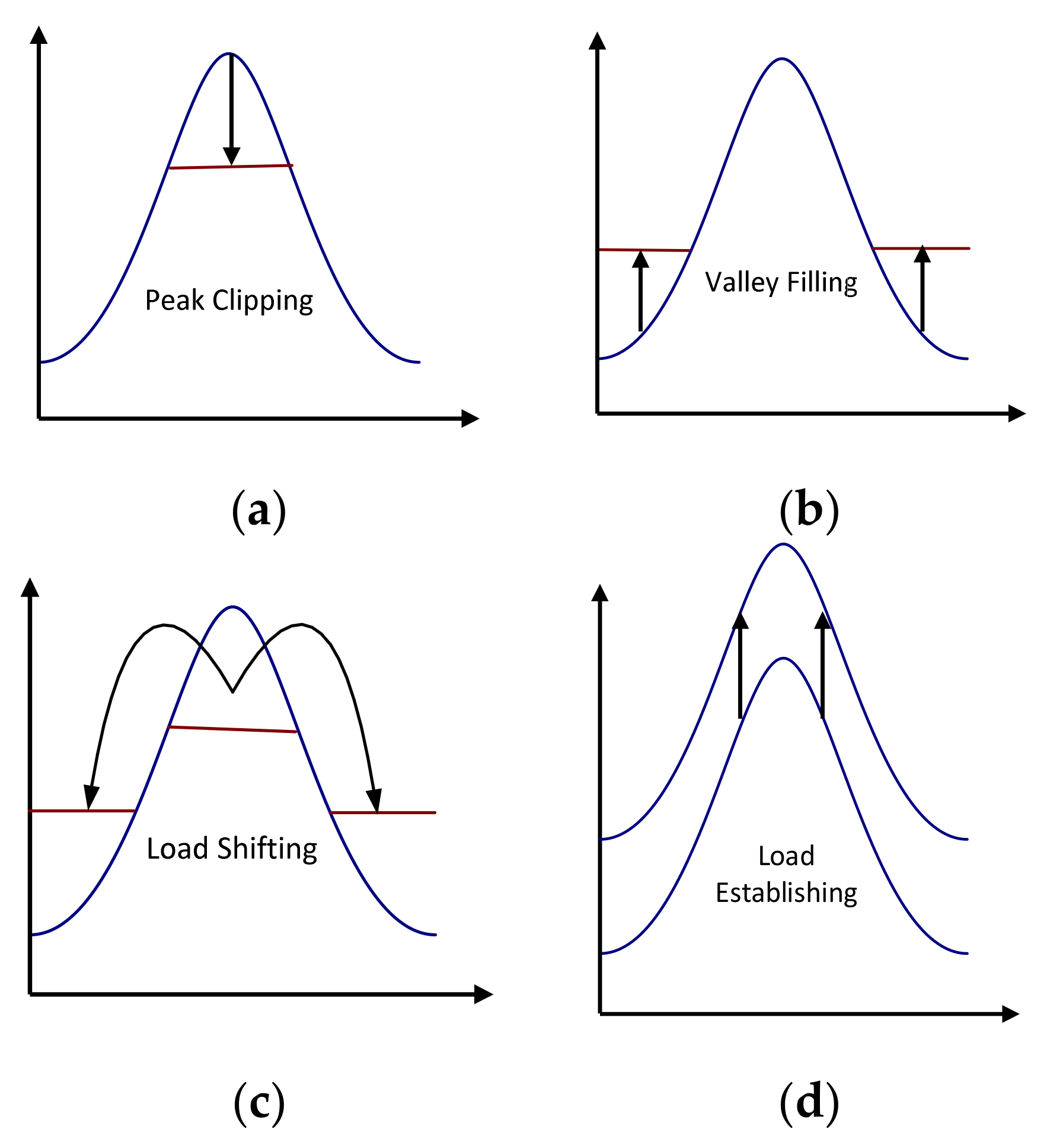
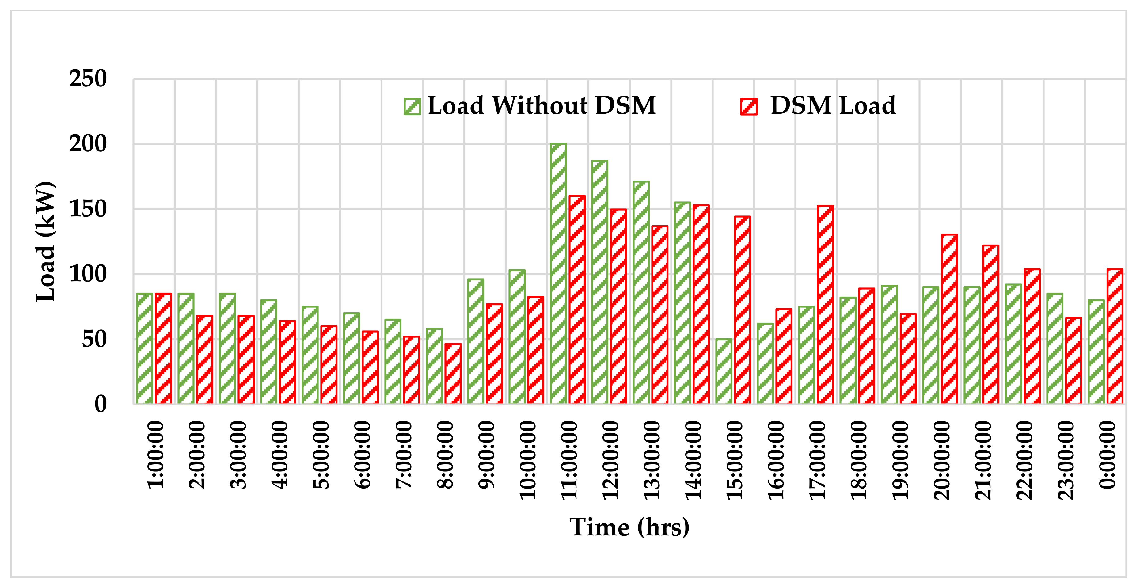
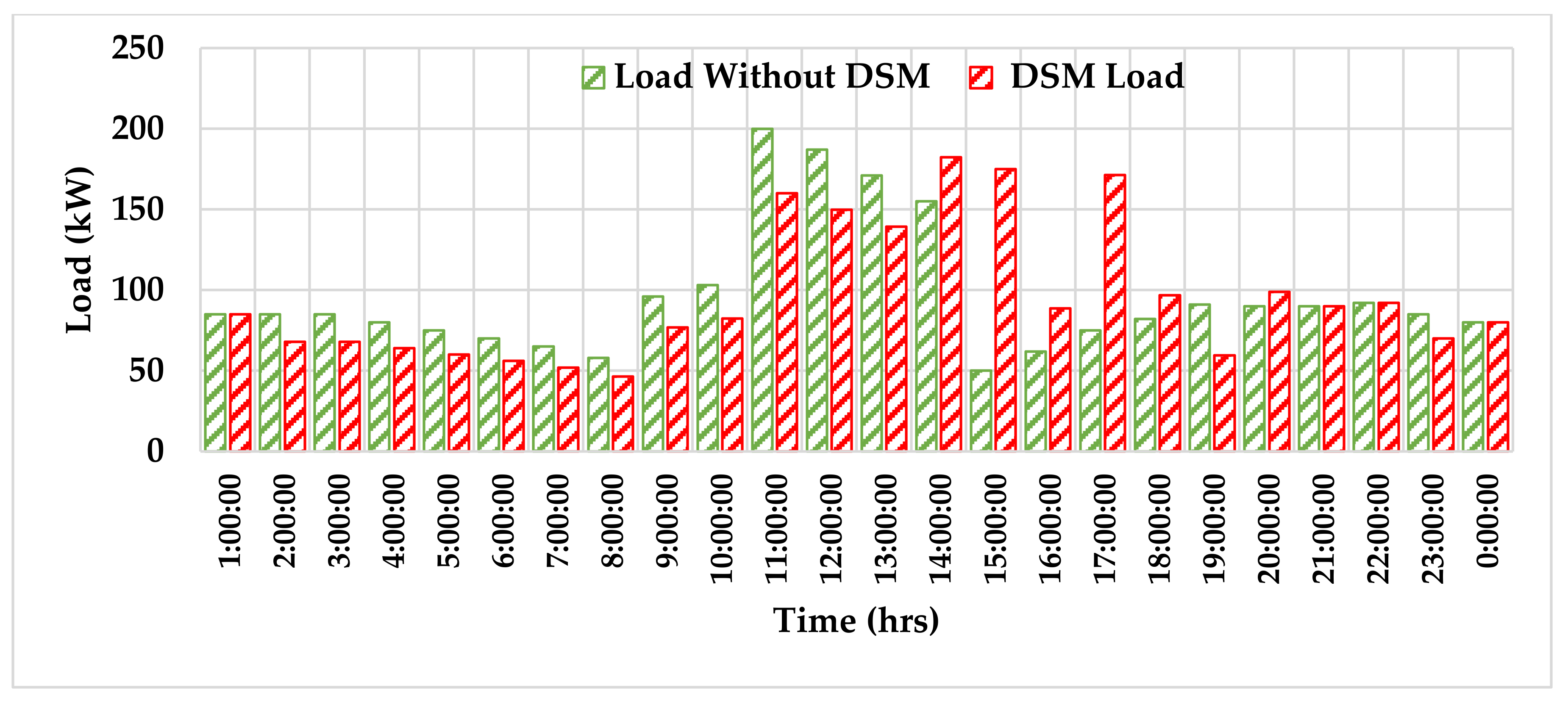
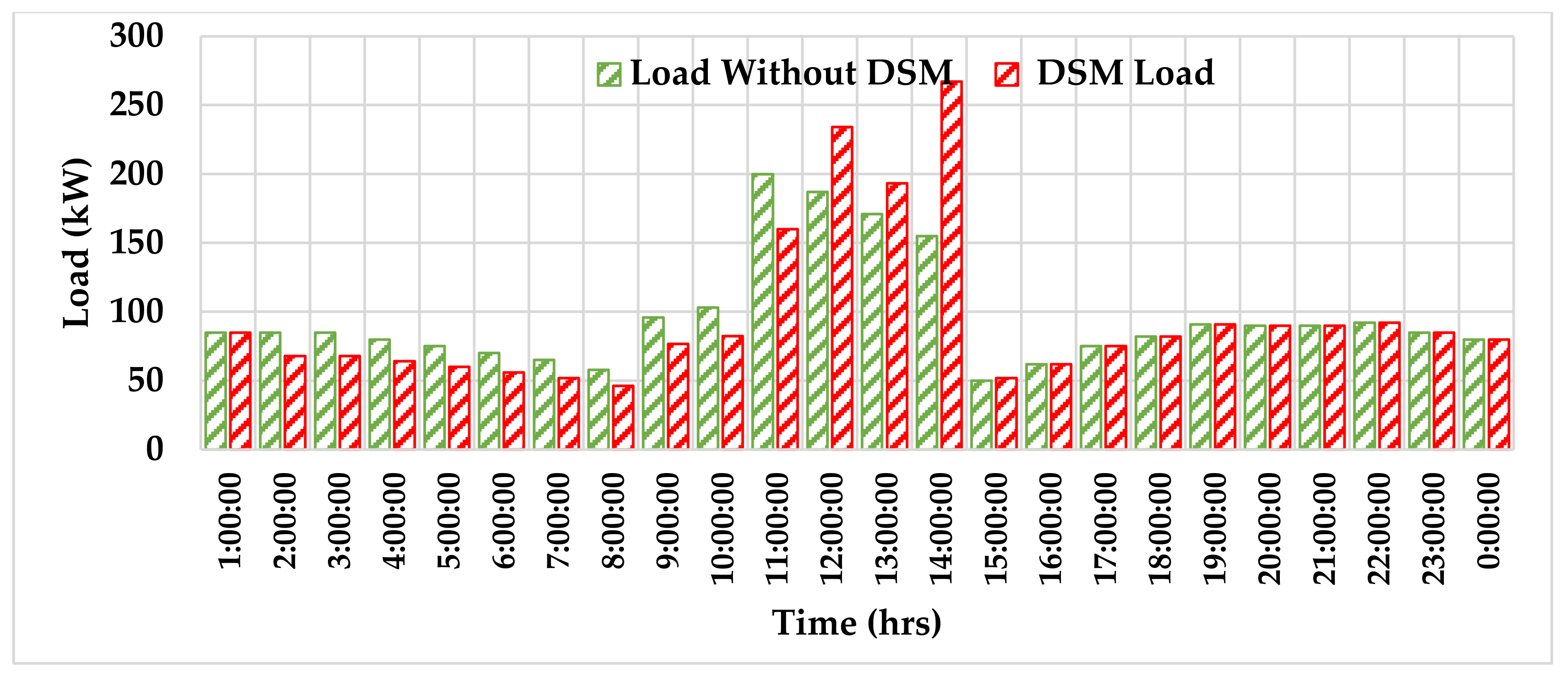
6. Demand Side Management (DSM)

Demand Side Management modifies the consumption patterns of consumer electricity to yield the desired alterations in the load structure of power distributions. The resulted changes are expected to reflect the planned objectives. This study presents a load-shifting technique to maximize the utilization of renewable energy resources and reduce the energy supply from the diesel. The objective load curve is aimed at reducing the load during periods of insufficient renewable energy and likewise increasing the load during periods of surplus renewable energy. The DSM strategy cannot be scheduled beyond a day, and the shifted load is limited to 20% of the total load. If the renewable energy is less than the load and within 24 h, as represented in (17), the load shift is described as (18). If (18) is greater than 20% of the load, the load shift is donated as (19). More so, by considering the future surplus available renewable energy, the load shift is limited to (20) if the available renewable energy is less than the expected shifted load in (19). The load at time, t , and future time, t + i , are represented as (21) and (22), respectively. The methodology also applies when there is surplus renewable energy.
P t + P w < P 1 t u n i v &   t < 24   h
l t = ( P 1 t u n i v P w t + P p t
l t = 0.2 P 1 t
l t = P r e n
P 1 t = P 1 t l t
P 1 t = P 1 t l t
where P t ,   P w ,   P 1 t ,   u n i v , P r e n , and l t represents PV power, wind power, load, inverter efficiency, surplus renewable energy, and load shift at time, t , respectively.

7. Reliability Indices

7.1. Loss of Power Supply Probability

The probability of power supply failure can be measured using one of the statistical reliability indices, Loss of Power Supply Probability (LPSP). Loss of power can be as a result of technical failure or low energy supply from the generating source that is not able to meet the demand [30]; 0% and 1% LPSP demonstrate, respectively, that the load will not be supplied and the load will be supplied. This can be calculated as described in (23) [35].
L P S P = P l o a d P p v P w i n d + P s o c m i n + P d i e s e l P l o a d
where P l o a d ,   P p v , P w i n d , P s o c m i n ,   a n d   P d i e s e l , are load demand, PV power, wind power, minimum battery power, and diesel power, respectively.

7.2. Renewable Energy Fraction (REF)

This is the ratio of diesel energy generated compared to energy generated from both the wind and the PV system, as shown below. The fraction is an indication of how much renewable energy is served. A fraction of 100% represents an ideal system, with only renewable energy resources. An equal sum of PV and wind power to diesel power represents a fraction of 0%. A fraction between 0% and 100% represent a hybrid energy source. REF is represented as (24) [29].
R E F = 1 P d i e s e l P w i n d + P p v 100

8. Objective Function

Appropriate sizing of the energy system with high quality units can lead to resourceful energy management and low-cost electricity for the consumers. The aim of the optimization is to obtain a minimal Cost of Energy (COE). COE is a widely used indicator for HES financial profitability [31]. This is defined as the ration of cost to unit price of electricity, as described in (25), subject to constraints (26) [29,35].
C O E $ k W h = A n n u a l i z e d   c o s t $ a n n u a l   e n e r g y   d e l i v e r e d   b y   t h e   s y s t e m   k W h = T o t a l   N e t   P r e s e n t   C o s t   $ P l o a d k W 8760 h y e a r C R F
Constraints   L P S P L P S P d e s i r e d R E F R E F d e s i r e d 0 P W i n d P w i n d , m a x 0 P p v P p v , m a x 0 P b a t P b a t , m a x 0 P D S L P D S L , m a x
The total NPC comprises installed capital costs. The installed capital costs includes the replacement cost, operation cost, maintenance cost, and present cost. P l o a d is the power consumed per hour. The current worth of HES components for a specific duration with the interest rate is calculated with the Capital Recovery Factor (CRF), which is shown below in (27) [35].
C R F = i 1 + i n 1 + i n 1
where n is the system life period, which is represented by PV life duration because of its lengthier life, and i represents interest rate. P w i n d , P p v , P D S L , and P b a t represent the rated power of wind, solar, diesel, and battery (in kWh), respectively, with their maximum denoted as P w i n d , m a x , P p v , m a x , P D S L , m a x , and P b a t , m a x . R E F d e s i r e d and L P S P d e s i r e d denote the defined REF and LPSP, respectively.

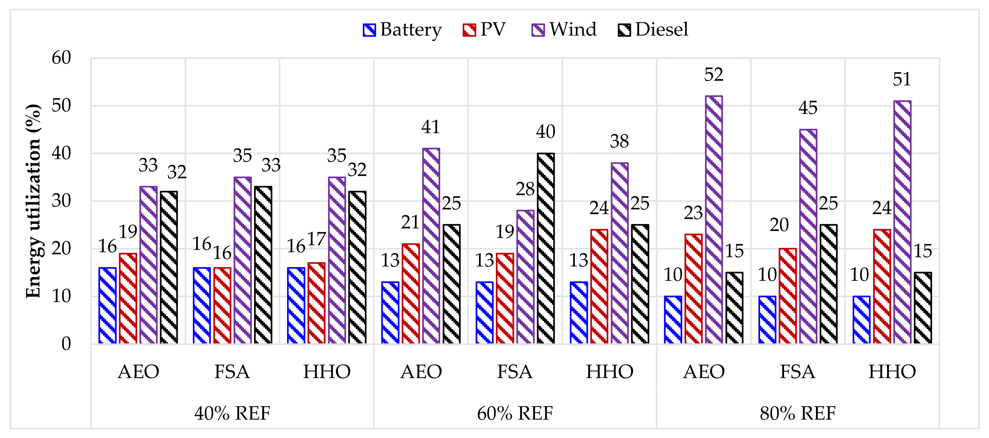
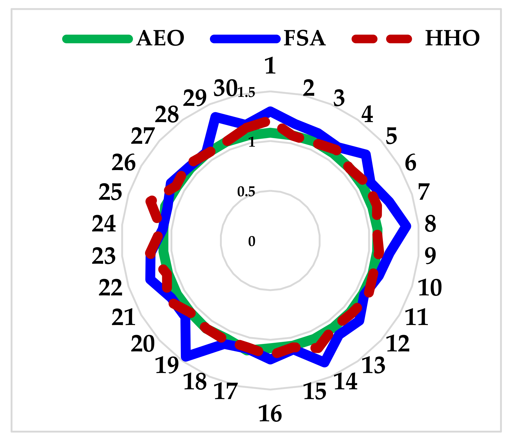
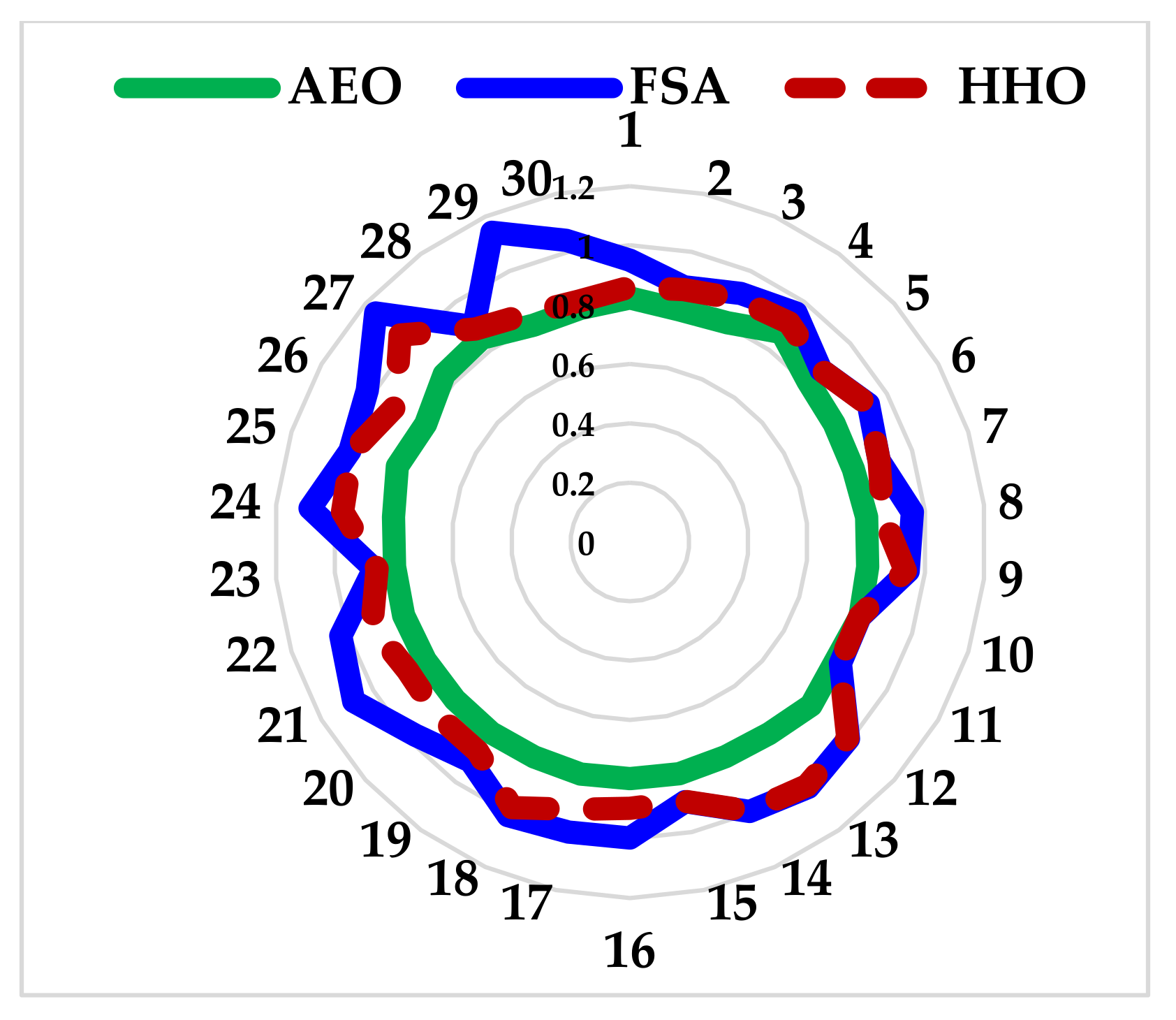
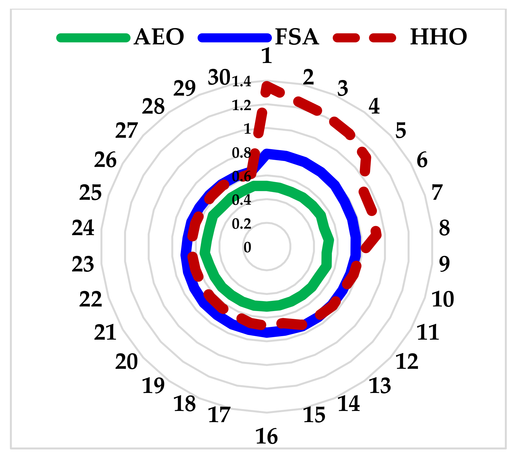
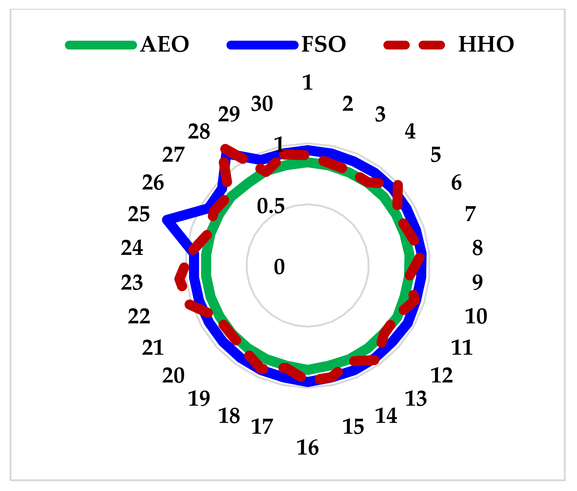
9. Simulation Results and Discussions

The proposed AEO, in addition to HHO and FSA, were employed to determine the optimal sizing of the stand-alone Hybrid Energy System to obtain the minimal Cost of Energy (COE). The hourly average load, wind speed, and solar irradiance of Al Sulaymaniyah village, Saudi Arabia, were selected for the study of optimal energy sizing in this study. The variables for the optimization are the capacity of the PV energy source, batteries, diesel generators, and wind turbine energy. The performance of the algorithms was evaluated under four performance indicators, which are Standard Deviation (STD), mean, best solution, and worst solution. The metaheuristics algorithm involves a stochastic model in their computational analysis. As a result, each run of the algorithm will not yield the same result. This creates an enormous challenge to determine the quality of the solution. Hence, it is crucial to investigate the consistency of the solution. By running the algorithms for 30 runs, a unique distinct pattern is obtained for the algorithms, which implies that the parameters always unite at a definite location. To obtain a rational comparison, the algorithms were evaluated under the same population sizes, iterations, boundary conditions, and number of runs. The simulation was developed using the MATLAB environment. Moreover, different levels of REF at 40%, 60%, and 80% at an LPSP of 0% were employed to achieve the COE and optimal sizing.

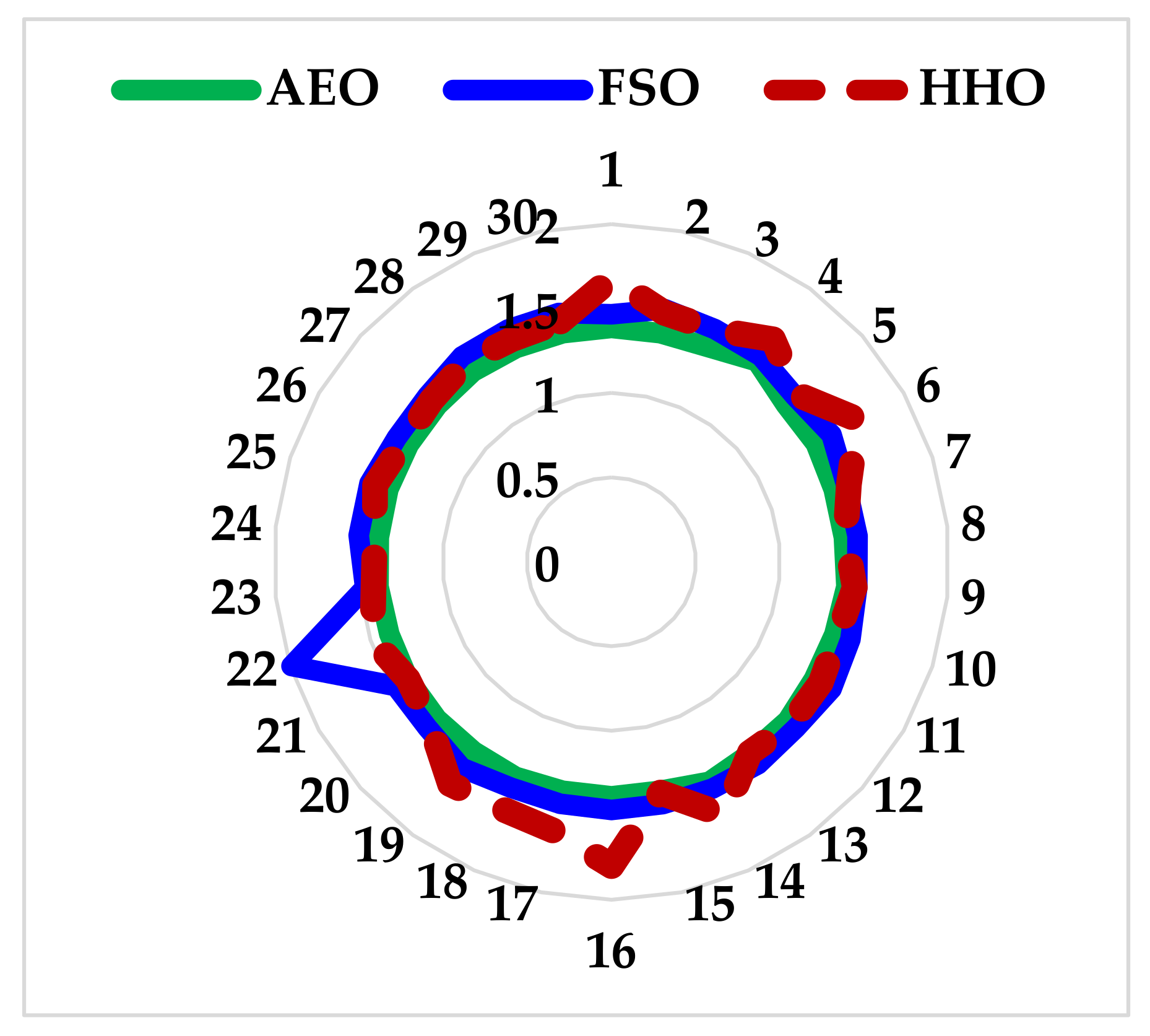
9.1. Optimal Sizing of the HES without DSM

One substantial standard for evaluating the performance of any optimization method is the assessment of the obtained fitness results. Table 2, Table 3 and Table 4 show the Standard Deviation (STD), mean, best solution, and worst solution obtained for REF at 40%, 60%, and 80%, respectively. These results were evaluated during 30 runs, 300 iterations, and a population size of 50 without DSM at 0% LPSP. Figure 7, Figure 8 and Figure 9 show the fitness curve of the three algorithms without DSM at 40%, 60%, and 80% REF, respectively. From the results, it is obvious that AEO obtained the minimum COE for all three stages. The algorithm further maintains a low STD value in obtaining the COE, as shown in Table 2, Table 3 and Table 4.
Figure 10 shows the percentage energy utilization for each of the algorithms without DSM. The run with the lowest COE for each algorithm was selected for the energy utilization plot. AEO utilizes the right combination of PV and wind energy sources to obtain the minimal cost of energy. Figure 10 shows that FSA utilizes the highest percentage for diesel energy. This influences its COE to be highest among the algorithms.

9.2. Optimal Sizing of the HES with DSM

The DSM is performed to optimize the usage of the available renewable energy resources. The loads are shifted in two categories: if there is insufficient renewable energy to meet the load or when there is surplus renewable energy. In the case of the surplus energy, future loads that are less than the available renewable energy are shifted to present time. All these load shifting are limited to a 24 h time frame. Table 5, Table 6 and Table 7 show the Standard Deviation (STD), mean, best solution, and worst solution obtained for 30 runs under 300 iterations and a population size of 50 for the three stages of Renewable Energy Fraction (REF). Figure 11, Figure 12 and Figure 13 show the fitness curve (COE) for the 30 runs of each algorithm at 40%, 60%, and 80% REF, respectively. It is obvious from Table 5, Table 6 and Table 7 and Figure 11, Figure 12 and Figure 13 that AEO achieved the minimal cost of energy at very low STD for all the 30 runs at 0% LPSP. This further demonstrates the ability of AEO to maintain the lowest COE with the highest consistent level and minimal STD.
Figure 14 shows the percentage energy utilization for each of the algorithms with DSM. The run with the lowest COE for each algorithm was selected for the energy utilization plot. From Table 5, Table 6 and Table 7 and Figure 11, Figure 12 and Figure 13, AEO utilizes the right combination of PV and wind energy sources to obtain the minimal cost of energy compared to the other algorithms. In the Figure, FSA utilizes the highest percentage for diesel energy. This influences its COE to be highest among the algorithms.

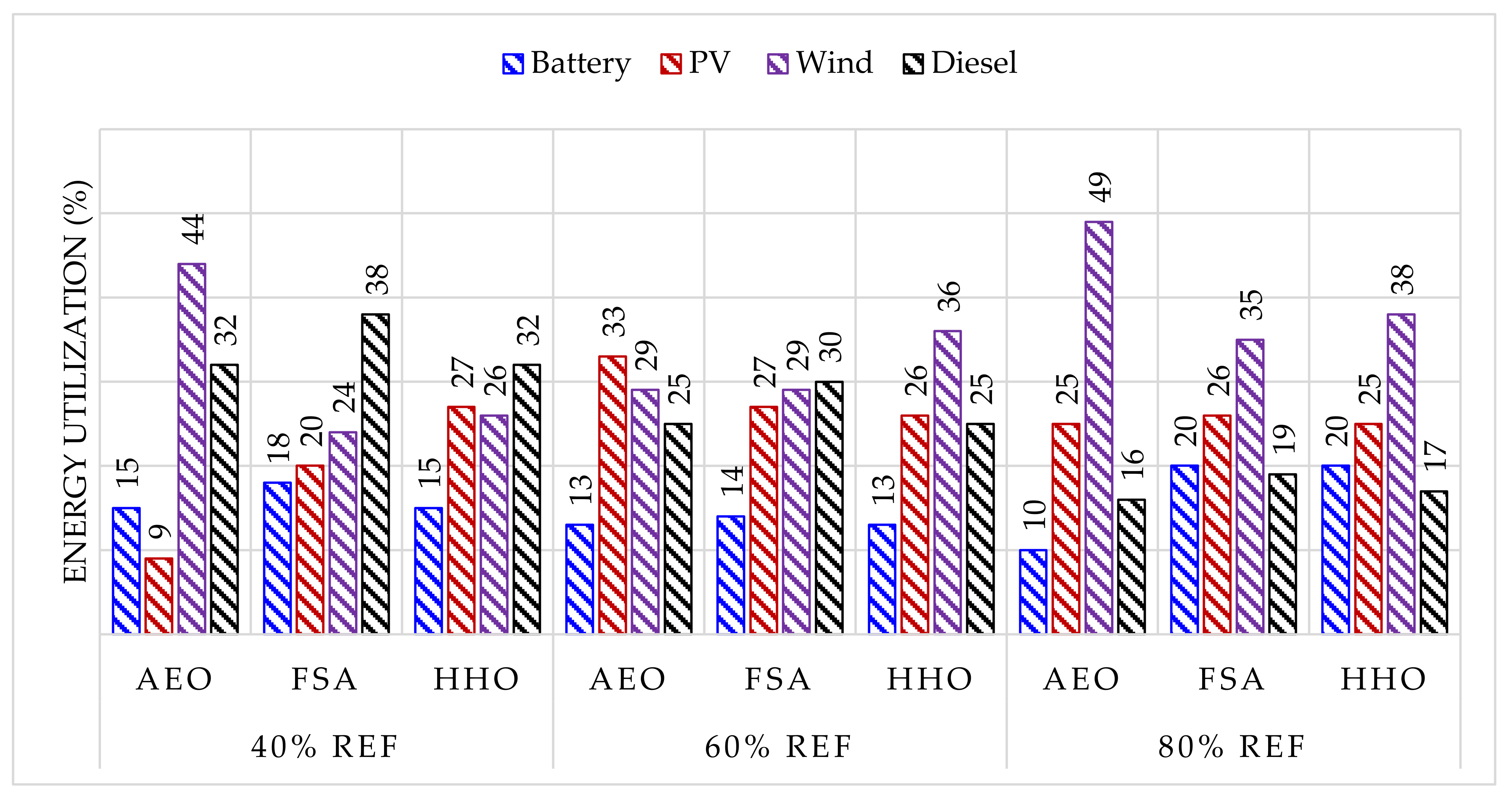
9.3. COE with DSM and without DSM

The DSM in this study is aimed at reducing the surplus renewable energy. Comparing the several results obtained, it can be observed that reducing the surplus energy decreases the COE. Because AEO produces the optimal results among the algorithms, Table 8 shows the percentage energy cost savings and COE at different REF when DSM is introduced as obtained from AEO. It can be observed that, with the introduction of DSM, greater energy saving is achieved. Figure 15, Figure 16 and Figure 17 show a typical one-day load profile for the AEO algorithm compared with and without Demand Side Management. The load profile shows how the surplus energy is utilized when there is low renewable energy and surplus renewable energy. In the figures, during the early hours of the day with low renewable energy supply, the loads are shifted to a later period in the day when there is a surplus renewable energy supply.

10. Conclusions

This paper presents a new application of AEO in the optimal sizing of a stand-alone Hybrid Energy System (HES). Al Sulaymaniyah, a rural area in Saudi Arabia, was selected for the optimal sizing of the HES. Cost of Energy (COE) was considered as the objective function of this model using both REF and LPSP as the reliability indices. Because of the abundance of renewable energy at the location, the optimal sizing selected both wind and solar energy as the major sources of energy. Furthermore, the optimal sizing was evaluated with and without Demand Side Management (DSM) under different Renewable Energy Fractions. It is obvious for both scenarios that AEO outperformed both HHO and FSA. By performing the DSM, more renewable energy was utilized while reducing the surplus unutilized energy. The DSM strategy achieved 28.38%, 43.05%, and 65.37% in COE saving at 40%, 60%, and 80% REF, respectively. The results stressed the importance of utilizing DSM for optimal sizing by further reducing the CEO. While the AEO algorithm introduced in this study has been shown to be efficient, it may not be efficient in other optimization problems. The efficacy of the algorithm can also be extended to the optimal load flow and optimal sitting of distributed generation.

Author Contributions

Conceptualization, H.O.O., A.M.A.-S. and A.A.A.-S.; methodology, H.O.O., A.A.A.-S. and H.M.H.F.; software, H.O.O.; validation, H.O.O., H.M.H.F. and A.A.A.-S.; formal analysis, H.O.O.; investigation, H.O.O.; resources, H.O.O. and A.A.A.-S.; data curation, H.O.O.; writing—original draft preparation, H.O.O.; writing—review and editing, H.O.O., A.M.A.-S., H.M.H.F. and A.A.A.-S.; visualization, H.O.O., A.M.A.-S., H.M.H.F. and A.A.A.-S.; supervision, H.O.O., A.M.A.-S., H.M.H.F. and A.A.A.-S.; project administration, H.O.O. and A.M.A.-S.; funding acquisition, A.M.A.-S. All authors have read and agreed to the published version of the manuscript.

Funding

This research received no external funding.

Acknowledgments

The authors would like to acknowledge the Researchers Supporting Project number (RSP-2021/337), King Saud University, Riyadh, Saudi Arabia.

Conflicts of Interest

The authors declare no conflict of interest.

Abbreviations

The following are abbreviations used.
AEOArtificial Ecosystem-based Optimization
COECost of Energy
CRFCapital Recovery Factor
DMOPSODynamic Multi-Objectives Particle Swarm Optimization
DSMDemand Side Management
FSA Future Search Optimization
HESHybrid Energy System
HHOHarris Hawk Optimization
HSHarmony Search
LOEELoss of Energy Expected
LOLELoss of Load Expected
LOLHLoss of Load Hours
LPSPLoss of Power Supply Probability
MPPMaximum Power Point
PFTPower Failure Time
REFRenewable Energy Fraction
RESRenewable Energy Resources
SOCState of Charge
STCsStandard Test Conditions
STDStandard Deviation
WTGWind Turbine Generator
aLinear weighting coefficient
A, BFuel constants
σTotal output power
αpPower temperature coefficient
CDslAnnual fuel consumption
CFCost of fuel per liter
DeDecomposer model
El(t)Total load demand
heWeight coefficients
G T ¯ Global irradiance under normal conditions
G T , S T C ¯ Global irradiance under STC
GT,NOCTSolar irradiance with respect to NOCT
fpvDe-rating factor
ηMPPMaximum Power Point (MPP) efficiency of PV module
ηMPP,STCEfficiency under STCs
ηinυNet inverter efficiency
ηbatteryRound trip efficiency of battery
NOCTOperating cell nominal temperature
LwLower boundary
ltLoad shift
PrPV rated power
PDsl(t)Generated power of diesel
PRNominal power
P t PV power
P w Wind power
P 1 t Load
PwindWind rated power
PpvRated solar power
PbatRated battery power
P r e n Surplus renewable energy
qPopulation number
r, r1Random number
Tc,STCPV temperatures under STC
TcPV temperatures under normal conditions
TaAmbient Temperature
Ta,NOCTAmbient temperature with respect to NOCT
weWeight coefficients
ucCut-in speed
urRated speed
xrandiRandom individual
UpUpper boundary
xqBest individual
ufCut-out frequency
univInverter efficiency

References

  1. Fekete, H.; Kuramochi, T.; Roelfsema, M.; Elzen, M.; den Forsell, N.; Höhne, N.; Luna, L.; Hans, F.; Sterl, S.; Olivier, J.; et al. A review of successful climate change mitigation policies in major emitting economies and the potential of global replication. Renew. Sustain. Energy Rev. 2021, 137, 110602. [Google Scholar] [CrossRef]
  2. Clausen, L.T.; Rudolph, D. Renewable energy for sustainable rural development: Synergies and mismatches. Energy Policy 2020, 138, 111289. [Google Scholar] [CrossRef]
  3. Alturki, F.A.; Omotoso, H.O.; Al-Shamma’a, A.A.; Farh, H.M.H.; Alsharabi, K. Novel Manta Rays Foraging Optimization Algorithm Based Optimal Control for Grid-Connected PV Energy System. IEEE Access 2020, 8, 187276–187290. [Google Scholar] [CrossRef]
  4. Al-Shamma’a, A.A.; Omotoso, H.O.; Noman, A.M.; Alkuhayli, A.A. Grey Wolf Optimizer Based Optimal Control for Grid-Connected PV System. In Proceedings of the IECON 2020 the 46th Annual Conference of the IEEE Industrial Electronics Society, Singapore, 19–21 October 2020; pp. 2863–2867. [Google Scholar]
  5. Ramesh, M.; Saini, R.P. Dispatch strategies based performance analysis of a hybrid renewable energy system for a remote rural area in India. J. Clean. Prod. 2020, 259, 120697. [Google Scholar] [CrossRef]
  6. Das, B.K.; Hassan, R.; Tushar, M.S.H.K.; Zaman, F.; Hasan, M.; Das, P. Techno-economic and environmental assessment of a hybrid renewable energy system using multi-objective genetic algorithm: A case study for remote Island in Bangladesh. Energy Convers. Manag. 2021, 230, 113823. [Google Scholar] [CrossRef]
  7. Das, M.; Singh, M.A.K.; Biswas, A. Techno-economic optimization of an off-grid hybrid renewable energy system using metaheuristic optimization approaches–Case of a radio transmitter station in India. Energy Convers. Manag. 2019, 185, 339–352. [Google Scholar] [CrossRef]
  8. Ramesh, M.; Saini, R. Demand Side Management based techno-economic performance analysis for a stand-alone hybrid renewable energy system of India. Energy Sources Part A Recover. Util. Environ. Eff. 2021, 1–29. [Google Scholar] [CrossRef]
  9. Lujano-Rojas, J.M.; Dufo-López, R.; Bernal-Agustín, J.L. Probabilistic modelling and analysis of stand-alone hybrid power systems. Energy 2013, 63, 19–27. [Google Scholar] [CrossRef]
  10. Alsayed, M.; Cacciato, M.; Scarcella, G.; Scelba, G. Design of hybrid power generation systems based on multi criteria decision analysis. Sol. Energy 2014, 105, 548–560. [Google Scholar] [CrossRef]
  11. Hung, D.Q.; Mithulananthan, N.; Bansal, R.C. Analytical strategies for renewable distributed generation integration considering energy loss minimization. Appl. Energy 2013, 105, 75–85. [Google Scholar] [CrossRef]
  12. Luna-Rubio, R.; Trejo-Perea, M.; Vargas-Vázquez, D.; Ríos-Moreno, G.J. Optimal sizing of renewable hybrids energy systems: A review of methodologies. Sol. Energy 2012, 86, 1077–1088. [Google Scholar] [CrossRef]
  13. Askarzadeh, A. Distribution generation by photovoltaic and diesel generator systems: Energy management and size optimization by a new approach for a stand-alone application. Energy 2017, 122, 542–551. [Google Scholar] [CrossRef]
  14. Sharafi, M.; ElMekkawy, T.Y. A dynamic MOPSO algorithm for multiobjective optimal design of hybrid renewable energy systems. Int. J. Energy Res. 2014, 38, 1949–1963. [Google Scholar] [CrossRef]
  15. Ghorbani, N.; Kasaeian, A.; Toopshekan, A.; Bahrami, L.; Maghami, A. Optimizing a hybrid wind-PV-battery system using GA-PSO and MOPSO for reducing cost and increasing reliability. Energy 2018, 154, 581–591. [Google Scholar] [CrossRef]
  16. Baghaee, H.R.; Mirsalim, M.; Gharehpetian, G.B.; Talebi, H.A. Reliability/cost-based multi-objective Pareto optimal design of stand-alone wind/PV/FC generation microgrid system. Energy 2016, 115, 1022–1041. [Google Scholar] [CrossRef]
  17. Koutroulis, E.; Kolokotsa, D.; Potirakis, A.; Kalaitzakis, K. Methodology for optimal sizing of stand-alone photovoltaic/wind-generator systems using genetic algorithms. Sol. Energy 2006, 80, 1072–1088. [Google Scholar] [CrossRef]
  18. Al-Shamma’a, A.A.; Addoweesh, K.E. Techno-economic optimization of hybrid power system using genetic algorithm. Int. J. Energy Res. 2014, 38, 1608–1623. [Google Scholar] [CrossRef]
  19. Kolhe, M.L.; Ranaweera, K.M.I.U.; Gunawardana, A.G.B.S. Techno-economic sizing of off-grid hybrid renewable energy system for rural electrification in Sri Lanka. Sustain. Energy Technol. Assess. 2015, 11, 53–64. [Google Scholar] [CrossRef]
  20. Wang, R.; Li, G.; Ming, M.; Wu, G.; Wang, L. An efficient multi-objective model and algorithm for sizing a stand-alone hybrid renewable energy system. Energy 2017, 141, 2288–2299. [Google Scholar] [CrossRef]
  21. Farh, H.M.H.; Al-Shaalan, A.M.; Eltamaly, A.M.; Al-Shamma’a, A.A. A novel severity performance index for optimal allocation and sizing of photovoltaic distributed generations. Energy Rep. 2020, 6, 2180–2190. [Google Scholar] [CrossRef]
  22. Farh, H.M.H.; Al-Shaalan, A.M.; Eltamaly, A.M.; Al-Shamma’A, A.A. A Novel Crow Search Algorithm Auto-Drive PSO for Optimal Allocation and Sizing of Renewable Distributed Generation. IEEE Access 2020, 8, 27807–27820. [Google Scholar] [CrossRef]
  23. Kaluthanthrige, R.; Rajapakse, A.D.; Lamothe, C.; Mosallat, F. Optimal Sizing and Performance Evaluation of a Hybrid Renewable Energy System for an Off-Grid Power System in Northern Canada. Technol. Econ. Smart Grids Sustain. Energy 2019, 4, 4. [Google Scholar] [CrossRef] [Green Version]
  24. Farh, H.M.H.; Eltamaly, A.M.; Al-Shaalan, A.M.; Al-Shamma’a, A.A. A novel sizing inherits allocation strategy of renewable distributed generations using crow search combined with particle swarm optimization algorithm. IET Renew. Power Gener. 2021, 15, 1436–1450. [Google Scholar] [CrossRef]
  25. Moslehi, K.; Kumar, R. A Reliability Perspective of the Smart Grid. IEEE Trans. Smart Grid 2010, 1, 57–64. [Google Scholar] [CrossRef]
  26. Logenthiran, T.; Srinivasan, D.; Khambadkone, A.M.; Aung, H.N. Multiagent System for Real-Time Operation of a Microgrid in Real-Time Digital Simulator. IEEE Trans. Smart Grid 2012, 3, 925–933. [Google Scholar] [CrossRef]
  27. Logenthiran, T.; Srinivasan, D.; Shun, T.Z. Demand Side Management in Smart Grid Using Heuristic Optimization. IEEE Trans. Smart Grid 2012, 3, 1244–1252. [Google Scholar] [CrossRef]
  28. Kumar, S.; Kaur, T.; Upadhyay, S.; Sharma, V.; Vatsal, D. Optimal Sizing of Stand Alone Hybrid Renewable Energy System with Load Shifting. Energy Sources Part A Recover. Util. Environ. Eff. 2020, 1–20. Available online: https://www.tandfonline.com/doi/full/10.1080/15567036.2020.1831107 (accessed on 8 November 2021). [CrossRef]
  29. Alturki, A.F.; Farh, M.H.H.; Al-Shamma’a, A.A.; Al Sharabi, K. Techno-Economic Optimization of Small-Scale Hybrid Energy Systems Using Manta Ray Foraging Optimizer. Electronics 2020, 9, 2405. [Google Scholar] [CrossRef]
  30. Zhao, W.; Wang, L.; Zhang, Z.; Al Sharabi, K. Artificial ecosystem-based optimization: A novel nature-inspired meta-heuristic algorithm. Neural Comput. Appl. 2020, 32, 9383–9425. [Google Scholar] [CrossRef]
  31. Elsisi, M.; Wang, L.; Zhang, Z.; Al Sharabi, K. Future search algorithm for optimization. Evol. Intell. 2019, 12, 21–31. [Google Scholar] [CrossRef]
  32. Heidari, A.A.; Mirjalili, S.; Faris, H.; Aljarah, I.; Mafarja, M.; Chen, H. Harris hawks optimization: Algorithm and applications. Futur. Gener. Comput. Syst. 2019, 97, 849–872. [Google Scholar] [CrossRef]
  33. Belfkira, R.; Zhang, L.; Barakat, G. Optimal sizing study of hybrid wind/PV/diesel power generation unit. Sol. Energy 2011, 85, 100–110. [Google Scholar] [CrossRef]
  34. Akhtari, M.R.; Baneshi, M. Techno-economic assessment and optimization of a hybrid renewable co-supply of electricity, heat and hydrogen system to enhance performance by recovering excess electricity for a large energy consumer. Energy Convers. Manag. 2019, 188, 131–141. [Google Scholar] [CrossRef]
  35. Borhanazad, H.; Mekhilef, S.; Gounder Ganapathy, V.; Modiri-Delshad, M.; Mirtaheri, A. Optimization of micro-grid system using MOPSO. Renew. Energy 2014, 71, 295–306. [Google Scholar] [CrossRef]
  36. Eid, A.; Kamel, S.; Korashy, A.; Khurshaid, T. An Enhanced Artificial Ecosystem-Based Optimization for Optimal Allocation of Multiple Distributed Generations. IEEE Access 2020, 8, 178493–178513. [Google Scholar] [CrossRef]
Figure 1. (a) Peak Clipping; (b) Valley Filling; (c) Load Shifting; (d) Load establishment.
Electronics 11 00204 g001
Figure 2. Al Sulaymaniyah village, Saudi Arabia.
Electronics 11 00204 g002
Figure 3. Overview of the proposed Hybrid Energy System.
Electronics 11 00204 g003
Figure 4. Wind turbine output power characteristics curve.
Electronics 11 00204 g004
Figure 5. Energy flow in an ecosystem.
Electronics 11 00204 g005
Figure 6. AEO ecosystem.
Electronics 11 00204 g006
Figure 7. Fitness for cost of energy without DSM at 40% REF and 0% LPSP.
Electronics 11 00204 g007
Figure 8. Fitness for cost of energy without DSM at 60% REF and 0% LPSP.
Electronics 11 00204 g008
Figure 9. Fitness for cost of energy without DSM at 80% REF and 0% LPSP.
Electronics 11 00204 g009
Figure 10. Energy utilization percent for AEO, FSA, and HHO without DSM and at 0% LPSP.
Electronics 11 00204 g010
Figure 11. Fitness for cost of energy with DSM at 40% REF and 0% LPSP.
Electronics 11 00204 g011
Figure 12. Fitness for cost of energy with DSM at 60% REF and 0% LPSP.
Electronics 11 00204 g012
Figure 13. AEO, FSA, and HHO Cost of Energy with DSM at 80% REF and 0% LPSP.
Electronics 11 00204 g013
Figure 14. Energy utilization percent for AEO, FSA, and HHO with DSM and at 0% LPSP.
Electronics 11 00204 g014
Figure 15. Daily load profile of AEO at 40% REF.
Electronics 11 00204 g015
Figure 16. Daily load profile of AEO at 60% REF.
Electronics 11 00204 g016
Figure 17. Daily load profile of AEO at 80% REF.
Electronics 11 00204 g017
Table 1. Parameters of the HES system.
ParametersValuesUnit
BatteryDepth of Discharge60%
Round-trip efficiency 80%
O&M Cost5USD/kWh/year
Capital cost200USD/kWh
Life span5years
Photovoltaic ModuleO&M Cost15USD/kW/year
Capital cost1000USD/kW
Efficiency16%
Life span20years
WTGHub-height60M
Cut-in/cut-off/ rated Speed3/25/9.5m/s
O&M Cost30.33USD/KW/year
Capital cost1300USD/kW
Life span20years
DC/AC ConverterLife span10years
Capital cost133USD/kW
Diesel GeneratorLife span15,000hours
Capital cost300USD/kW
O&M Cost0.012USD/kWh
Project FactorsInterest rate3%
Life span20years
Inflation rate2%
Table 2. Optimal, Minimum, Maximum, and STD for AEO, FSA, and HHO at 40% REF and LPSP of 0%.
COE (USD/kWh)Pbatt (kW)PV (kW)Pw (kW)Pdiesel (kW)Surplus (%)
AEOOptimal1.38363062.46167.98102.14168.5635.05
Mean1.39306659.96154.99108.26168.5035.82
Max1.46719761.5381.25142.95171.0140.19
STD0.01636210.0325.0810.711.291.11
FSAOptimal1.4636500.00166.14111.88164.8836.17
Mean1.50050134.71161.68109.69167.8837.12
Max1.99324237.52156.82109.91166.1140.00
STD0.2362228.8967.4019.138.764.07
HHOOptimal1.39213860.77147.83110.09168.3535.32
Mean1.50015457.73122.63123.51173.2238.55
Max1.79933447.347.50190.97189.5151.14
STD0.10605826.0165.8629.476.334.05
Table 3. Optimal, Minimum, Maximum, and STD for AEO, FSA, and HHO at 60% REF and LPSP of 0%.
COE (USD/kWh)Pbatt (kW)PV (kW)Pw (kW)Pdiesel (kW)Surplus (%)
AEOOptimal1.13368969.55190.20129.39162.2639.27
Mean1.14394265.13180.08135.52162.0040.39
Max1.20679950.35102.23177.15162.2646.53
STD0.0164468.8028.9714.171.001.83
FSAOptimal1.13422766.36185.97131.59161.8240.39
Mean1.15410927.32198.22133.23159.8541.24
Max1.1772330.00250.00118.59159.4139.19
STD0.01571331.7319.067.211.662.11
HHOOptimal1.13824156.38211.12123.02161.4839.65
Mean1.20639862.38157.37146.20165.0042.25
Max1.5961428.8139.77190.56175.8750.89
STD0.09544929.0758.0926.115.463.37
Table 4. Optimal, Minimum, Maximum, and STD for AEO, FSA, and HHO at 80% REF and LPSP of 0%.
COE (USD/kWh)Pbatt (kW)PV (kW)Pw (kW)Pdiesel (kW)Surplus (%)
AEOOptimal0.83223571.22244.09189.75150.2049.71
Mean0.83748766.17224.90200.15149.7851.3
Max0.85371063.39178.53225.41149.4853.77
STD0.00477310.1418.059.251.232.53
FSAOptimal1.224227 75.22200.09180.75123.2048.71
Mean1.24703860.17221.90210.15159.7850.3
Max1.33675060.39188.53221.42159.2853.77
STD0.234455 22.4167.0529.258.233.13
HHOOptimal0.83561374.05239.33190.54150.5649.61
Mean0.92277973.36203.67190.57155.0547.8
Max1.70210478.2511.09199.96189.0344.47
STD0.15613020.1953.9911.747.852.33
Table 5. Optimal, Minimum, Maximum, and STD for AEO, FSA, and HHO with DSM at 40% REF and 0% LPSP.
COE (USD/kWh)Pbatt (kW)PV (kW)Pw (kW)Pdiesel (kW)Surplus (%)
AEOOptimal1.07772322.41228.1562.25143.7329.24
Mean1.11916341.46164.2486.23149.9429.93
Max1.26786658.4850.08139.18159.4437.23
STD0.04736612.6850.3621.673.682.59
FSAOptimal1.08736926.59220.2964.32144.4028.94
Mean1.19567810.33215.9768.28143.4830.38
Max1.44521857.70129.5698.27153.3129.84
STD0.09263316.5077.7331.4612.795.96
HHOOptimal1.08736916.40202.6271.30144.8129.43
Mean1.19928853.89123.47103.10156.1332.11
Max1.44521841.3811.77154.75168.2041.77
STD0.09165224.7767.1429.997.484.23
Table 6. Optimal, Minimum, Maximum, and STD for AEO, FSA, and HHO with DSM at 60% REF and 0% LPSP.
COE (USD/kWh)Pbatt (kW)PV (kW)Pw (kW)Pdiesel (kW)Surplus (%)
AEOOptimal0.79249429.27247.0476.52127.8529.27
Mean0.81108037.90208.5990.92132.0937.90
Max0.92218664.8491.04146.83144.3864.84
STD0.02746815.0135.7815.933.783.01
FSAOptimal0.81632159.17217.0579.51117.4530.17
Mean0.96223637.90208.5990.92132.0936.91
Max1.15281961.8591.12136.13124.1866.81
STD0.09288915.0135.7815.933.786.02
HHOOptimal0.81432059.70128.63127.71143.4830.45
Mean0.91023459.70128.63127.71143.4835.15
Max1.115856101.2519.23191.81160.8035.17
STD0.06820024.9552.2927.796.515.12
Table 7. Optimal, Minimum, Maximum, and STD for AEO, FSA, and HHO with DSM at 80% REF and 0% LPSP.
COE (USD/kWh)Pbatt (kW)PV (kW)Pw (kW)Pdiesel (kW)Surplus (%)
AEOOptimal0.50324537.28242.48123.52106.5836.50
Mean0.51162836.54215.42136.24108.4337.82
Max0.52874633.89171.15159.52110.7041.07
STD0.00726817.7422.4910.572.361.42
FSAOptimal0.64427574.29217.11199.87125.8750.0
Mean0.64427577.73172.01192.91147.8146.33
Max0.78175090.5121.71209.00138.4842.66
STD0.31960419.9470.919.0912.904.3
HHOOptimal0.62712554.28247.16196.86135.8649.83
Mean0.78785878.79176.08194.92147.8445.34
Max1.35308289.5020.70200.00178.4841.65
STD0.21737018.9374.908.0611.893.3
Table 8. Percentage energy cost saving and COE at different REF.
REF (%)COE with DSM (USD/kWh)Surplus Energy with DSM (%)COE without DSM (USD/kWh)Surplus Energy without DSM (%)Percentage Energy Cost Saving (%)
401.07772329.241.3836335.0528.38
600.79249429.271.13368939.2743.05
800.50324536.50.83223549.7165.37
Publisher’s Note: MDPI stays neutral with regard to jurisdictional claims in published maps and institutional affiliations.

